

Page 1

User´s Guide
LXG cameras with Visual Applets
(Gigabit Ethernet)
Document Version: v1.1
Release: 06.04.16
Document Number: 11162763
Page 2

2
Page 3

3
Table of Contents
1. General Information ................................................................................................. 6
2. General safety instructions ..................................................................................... 7
3. Intended Use ............................................................................................................. 7
4. General Description ................................................................................................. 7
5. Camera Models ......................................................................................................... 8
5.1 LXG – Cameras with Visual Applets ....................................................................... 8
5.2 Lens Mount Adapter .............................................................................................. 10
5.3 Flange Focal Distance .......................................................................................... 12
6. Installation .............................................................................................................. 12
6.1 Environmental Requirements ................................................................................ 12
6.2 Heat Transmission ................................................................................................ 13
6.3 Mechanical Tests ................................................................................................... 14
7. Process- and Data Interface .................................................................................. 15
7.1 Pin-Assignment Interface ...................................................................................... 15
7.2 Pin-Assignment Power Supply and Digital-IOs ..................................................... 15
7.3 LED Signaling ....................................................................................................... 16
8. ProductSpecications .......................................................................................... 17
8.1 Sensor Specications ........................................................................................... 17
8.1.1 Quantum Efciency for Baumer LXG - Cameras with Visual Applets ............. 17
8.1.2 Shutter ............................................................................................................ 18
8.1.3 Digitization Taps ............................................................................................ 18
8.1.4 Field of View Position ..................................................................................... 19
8.2 Timings .................................................................................................................. 20
8.2.1 Free Running Mode ........................................................................................ 20
8.2.2 Trigger Mode .................................................................................................. 21
9. Software .................................................................................................................. 25
9.1 Baumer GAPI SDK ............................................................................................... 25
9.2 3rd Party Software .................................................................................................. 25
10. Camera Functionalities .......................................................................................... 26
10.1 Image Acquisition ................................................................................................ 26
10.1.1 Image Format ............................................................................................... 26
10.1.2 Pixel Format ................................................................................................. 27
10.1.3 Exposure Time.............................................................................................. 29
10.1.4 PRNU / DSNU Correction (FPN - Fixed Pattern Noise) ............................... 29
10.1.5 HDR .............................................................................................................. 30
10.1.6 Region of Interest (ROI) ............................................................................... 31
Page 4

4
10.2 Analog Controls ................................................................................................... 33
10.2.1 Offset / Black Level ....................................................................................... 33
10.2.2 Gain .............................................................................................................. 33
10.3 Defect Pixel Correction ....................................................................................... 33
10.3.1 General information ...................................................................................... 33
10.3.2 Correction Algorithm ..................................................................................... 34
10.3.3 DefectPixelList .............................................................................................. 34
10.4 Sequencer ........................................................................................................... 35
10.4.1 General Information ...................................................................................... 35
10.4.2 Baumer Optronic Sequencer in Camera xml-le .......................................... 36
10.4.3 Examples ...................................................................................................... 36
10.4.4 Capability Characteristics of Baumer GAPI Sequencer Module .................. 37
10.4.5 Double Shutter ............................................................................................. 38
10.5 Process Interface ................................................................................................ 39
10.5.1 Digital I/O ...................................................................................................... 39
10.6 Trigger Input / Trigger Delay ............................................................................... 41
10.6.1 Trigger Source .............................................................................................. 42
10.6.2 Debouncer .................................................................................................... 43
10.6.3 Flash Signal .................................................................................................. 43
10.6.4 Timer............................................................................................................. 44
10.7 User Sets ............................................................................................................ 45
10.8 Factory Settings .................................................................................................. 45
11. Interface Functionalities ........................................................................................ 46
11.1 Device Information .............................................................................................. 46
11.2 Baumer Image Info Header (Chunk Data)........................................................... 47
11.3 Packet Size and Maximum Transmission Unit (MTU) ......................................... 48
11.4 "Inter Packet Gap" (IPG) .................................................................................... 49
11.4.1 Example 1: Multi Camera Operation – Minimal IPG ..................................... 49
11.4.2 Example 2: Multi Camera Operation – Optimal IPG ..................................... 50
11.5 Frame Delay ........................................................................................................ 51
11.5.1 Time Saving in Multi-Camera Operation ....................................................... 51
11.5.2 Conguration Example ................................................................................. 52
11.6 Multicast .............................................................................................................. 54
11.7 IP Conguration ................................................................................................... 55
11.7.1 Persistent IP ................................................................................................. 55
11.7.2 DHCP (Dynamic Host Conguration Protocol) ............................................. 55
11.7.3 LLA ................................................................................................................ 56
11.7.4 Force IP ........................................................................................................ 56
11.8 Packet Resend .................................................................................................... 57
11.8.1 Normal Case ................................................................................................. 57
11.8.2 Fault 1: Lost Packet within Data Stream ....................................................... 57
11.8.3 Fault 2: Lost Packet at the End of the Data Stream ..................................... 58
11.8.4 Termination Conditions ................................................................................ 58
11.9 Message Channel ............................................................................................... 59
11.10 Action Commands ............................................................................................. 60
11.10.1 Action Command Trigger ............................................................................ 60
12. Start-Stop-Behaviour ............................................................................................. 61
12.1 Start / Stop Acquisition (Camera) ........................................................................ 61
12.2 Start / Stop Interface ........................................................................................... 61
12.3 Pause / Resume Interface .................................................................................. 61
12.4 Acquisition Modes ............................................................................................... 61
Page 5

5
12.4.1 Free Running ................................................................................................ 61
12.4.2 Trigger .......................................................................................................... 61
12.4.3 Sequencer .................................................................................................... 61
13. Cleaning .................................................................................................................. 62
13.1 Sensor ................................................................................................................. 62
13.2 Cover glass ......................................................................................................... 62
13.3 Housing ............................................................................................................... 62
14. Transport / Storage ................................................................................................ 63
15. Disposal .................................................................................................................. 63
16. Warranty Information ............................................................................................. 63
17. Conformity .............................................................................................................. 64
17.1 CE ....................................................................................................................... 64
18. Support .................................................................................................................... 64
Page 6

6
1. General Information
Thanks for purchasing a camera of the Baumer family. This User´s Guide describes how
to connect, set up and use the camera.
Read this manual carefully and observe the notes and safety instructions!
Target group for this User´s Guide
This User's Guide is aimed at experienced users, which want to integrate camera(s) into
a vision system.
Copyright
Any duplication or reprinting of this documentation, in whole or in part, and the reproduc-
tion of the illustrations even in modied form is permitted only with the written approval of
Baumer. This document is subject to change without notice.
Classicationofthesafetyinstructions
In the User´s Guide, the safety instructions are classied as follows:
Notice
Gives helpful notes on operation or other general recommendations.
Caution
Pictogram
Indicates a possibly dangerous situation. If the situation is not avoided,slight
or minor injury could result or the device may be damaged.
Page 7

7
2. General safety instructions
Observe the the following safety instruction when using the camera to avoid any damage
or injuries.
Caution
Provide adequate dissipation of heat, to ensure that the temperature does
not exceed +50 °C (+122 °F).
The surface of the camera may be hot during operation and immediately
after use. Be careful when handling the camera and avoid contact over a
longer period.
3. Intended Use
The camera is used to capture images that can be transferred over a GigE interface to a
PC.
Notice
Use the camera only for its intended purpose!
For any use that is not described in the technical documentation poses dangers and will
void the warranty. The risk has to be borne solely by the unit´s owner.
4. General Description
1
2
3
4
5
No. Description No. Description
1
LXG-40M.P
C-Mount only.
LXG-120M.P / LXG-200M.P
lens mount (M58), adapter for
other lens mounts available
4 Signaling LED
2 Data Port 1 (PoE) 5 Digital-IO (RS485)
3 Power Suppy / Digital-IO
Page 8

8
5. Camera Models
5.1 LXG – Cameras with Visual Applets
LXG-40M.P
LXG-120M.P
LXG-200M.P
Camera Type
Sensor
Size
Resolution
Full Frames
[max. fps]
Monochrome / Color
LXG-40M.P 1" 2048 x 2048 74
LXG-120M.P APS-C 4096 x 3072 25
LXG-200M.P 35 mm 5120 x 3840 16
Page 9
9
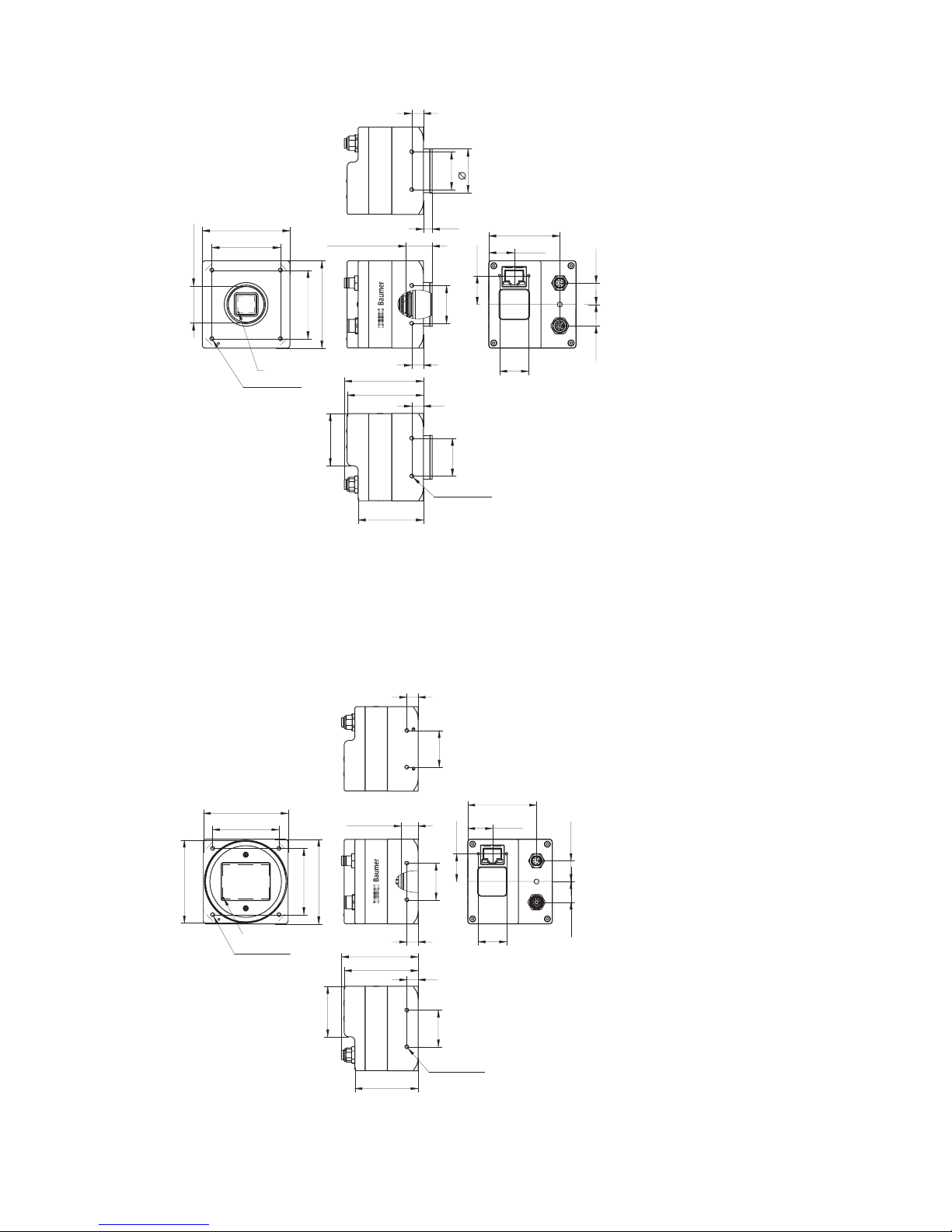
Dimensions
60
604747
Pixel 0,0
8 x M3 x 6
1"-32 UN
18,055 ±0,025
26
8
52,35
54,25
44,75
8
26
8 x M3 x 6
8
26
30
6
19,7
20
17,5
48,8
14,7
14,7
35,8
LXG-40M.P
47
60
47
60
M58 x 0,75
Pixel 0,0
4 x M3 x 6
44,75
52,35
54,25
35,8
8
26
8 x M3 x 6
8
26
12 ±0 ,25
8
26
14,7
19,7
20
17,5
48,8
14,7
LXG-120M.P
LXG-200M.P
◄Figure1
Dimensions of the Baumer LXG cameras with
Visual Applets
Page 10

10
5.2 Lens Mount Adapter
Notice
LXG-40M.P have a C-Mount interface only.
Adapter M58 / F-Mount (Art. No.: 11117852)
59ø
40,43
F-Mount
M58x0,75
Adapter M58 / M42x1-Mount (26.8mm) (Art. No.: 11127232)
20,75
59ø
M58x0,75
M42x1
3
ø
50
Notice
suitable for Zeiss M42 lenses (e.g. Biogon T* 2.8/21 Z-M42-I, Biogon T* 2/35 Z-M42-I,
C Sonnar T* 1.5/50 Z-M42-I)
Page 11

11
Adapter M58 / M42x1-MOUNT (45.5 mm) (Art. No: 11137781)
39,43
59ø
M58x0,75
M42x1
3
ø
50
Notice
suitable for Zeiss (e.g. Distagon T* 2/25 Z-M42-I, Planar T* 1.4/50 Z-M42-I, MakroPlanar T* 2/50 Z-M42-I) and KOWA M42 lenses (e.g. LM28LF P-Mount, LM35LF
P-Mount)
Adapter M58 / C-Mount (Art. No: 11115198)
C-Mount
M58x0,75
59ø
30ø
4,467
3ø
50
Page 12

12
5.3 Flange Focal Distance
12 ±0,25
6. Installation
Lens mounting
Notice
Avoid contamination of the sensor and the lens by dust and airborne particles when
mounting the support or the lens to the device!
Therefore the following points are very important:
▪ Install the camera in an environment that is as dust free as possible!
▪ Keep the dust cover (foil) on camera as long as possible!
▪ Hold the print with the sensor downwards with unprotected sensor.
▪ Avoid contact with any optical surface of the camera!
6.1 Environmental Requirements
Temperature
Storage temperature -10 °C ... +70 °C ( +14 °F ... +158 °F)
Operating temperature* see Heat Transmission
* If the environmental temperature exceeds the values listed in the table below, the cam-
era must be cooled. (see Heat Transmission)
Humidity
Storage and Operating Humidity 10 % ... 90 %
Non-condensing
Page 13

13
6.2 Heat Transmission
Caution
Provide adequate dissipation of heat, to ensure that the temperature does
not exceed +50 °C (+122 °F) at temperature measurment point T.
The surface of the camera may be hot during operation and immediately
after use. Be careful when handling the camera and avoid contact over a
longer period.
As there are numerous possibilities for installation, Baumer do not speciy
a specic method for proper heat dissipation, but suggest the following prin-
ciples:
▪ operate the cameras only in mounted condition
▪ mounting in combination with forced convection may provide proper heat
dissipation
T
T
Measure Point Maximal Temperature
T 50°C (122°F)
For remote temperature monitoring of the camera a temperature sensor is integrated.
Notice
The temperature sensor is able to deliver values of 0°C (32°F) to +85°C (185°F)
Take care that the temperature of the camera does not exceed the specied case temperature +50°C (+122°F).
◄Figure2
Temperature measure-
ment points of Baumer
LXG cameras with Visual Applets.
Page 14

14
6.3 Mechanical Tests
Tested with C-Mount adapter adapter and lens dummy.
Environmental
Testing
Standard Parameter
Vibration,
sinussodial
IEC 60068-2-6 Search for
Resonance
10-2000 Hz
Amplitude underneath crossover frequencies
0,75 mm
Acceleration 1 g
Test duration 15 min (axis)
45 min (total)
Vibration, broad
band
IEC 60068-2-64 Frequency
range
10-1000 Hz
Acceleration 10 g
Test duration 300 min (axis)
15 h (total)
Shock IEC 60068-2-27 Puls time 11 ms / 6 ms
Acceleration 50 g / 100 g
Bump IEC60068-2-29 Pulse Time 2 ms
Acceleration 100 g
Page 15

15
7. Process- and Data Interface
7.1 Pin-Assignment Interface
Notice
The Data Port supports Power over Ethernet (36 VDC .. 57 VDC).
Data / Control 1000 Base-T
LED2
LED1
8
1
1 MX1+ (green/white)
(negative/positive V
port
)
5 MX3- (blue/white)
2 MX1- (green)
(negative/positive V
port
)
6 MX2- (orange)
(positive/negative V
port
)
3 MX2+ (orange/white)
(positive/negative V
port
)
7 MX4+ (brown/white)
4 MX3+ (blue) 8 MX4- (brown)
7.2 Pin-Assignment Power Supply and Digital-IOs
Power and Process Interface #1
(SACC-DSI-M8FS-8CON-M10-L180 SH)
Power and Process Interface #2
(SACC-DSI-M8MS-8CON-M8-L180 SH)
M8 / 8 pins wire colors of the connecting cable
8
5
7
3
1
4
2
6
8
5
7
3
1
4
2
6
1 white OUT 3 (line 3) 1 white In2_RS485+ (line4)
2 brown Power VCC+ 2 brown In2_RS485- (line4)
3 green IN 1 (line 0) 3 green In2_RS485+ (line5)
4 yellow IO GND 4 yellow In2_RS485- (line5)
5 grey IO Power VCC 5 grey OUT3_In2_RS485+ (line6)
6 pink OUT 1 (line 1) 6 pink OUT3_In2_RS485- (line6)
7 blue Power GND 7 blue external Power GND
8 red OUT 2 (line 2) 8 red external Power 5 V/200 mA
Power Supply
Power VCC 12 VDC ... 24 VDC
Page 16

16
7.3 LED Signaling
LED
Signal Meaning
Camera LED
green on Power on, link good
green blinking Power on, no link
red on Error
red blinking
Warning
(update in progress, don’t switch off)
yellow Readout active
Figure3►
LED positions on Baumer LXG
cameras.
Page 17

17
8. ProductSpecications
8.1 SensorSpecications
8.1.1 QuantumEfciencyforBaumerLXG-CameraswithVisualApplets
The quantum efciency characteristics of Baumer LXG - cameras with Visual Applets are
displayed in the following graphs. The characteristic curves for the sensors do not take
the characteristics of lenses and light sources without lters into consideration, but are
measured with an AR coated cover glass.
Values relating to the respective technical data sheets of the sensors manufacturer.
350 450 550 650 750 850 950 1050
Wave Length [nm]
Quantum Efficiency [%]
LXG-40M.P
MonoMono
350 450 550 650 750 850 950 1050
Wave Length [nm]
Quantum Efficiency [%]
LXG-120M.P
Mono
350 450 550 650 750 850 950 1050
Wave Length [nm]
Quantum Efficiency [%]
LXG-200M.P
Mono
◄Figure4
Quantum efciency for
Baumer LXG cameras
with Visual Applets.
Page 18
18
8.1.2 Shutter
All cameras of the LXG - camera with Visual Applets series are equipped with a global
shutter.
Pixel
Active Area (Photodiode)
Storage Area
Microlens
Global shutter means that all pixels of the sensor are reset and afterwards exposed for a
specied interval (t
exposure
).
For each pixel an adjacent storage circuit exists. Once the exposure time elapsed, the
information of a pixel is transferred immediately to its circuit and read out from there.
Due to the fact that photosensitive area gets "lost" by the implementation of the circuit
area, the pixels are equipped with microlenses, which focus the light on the pixel.
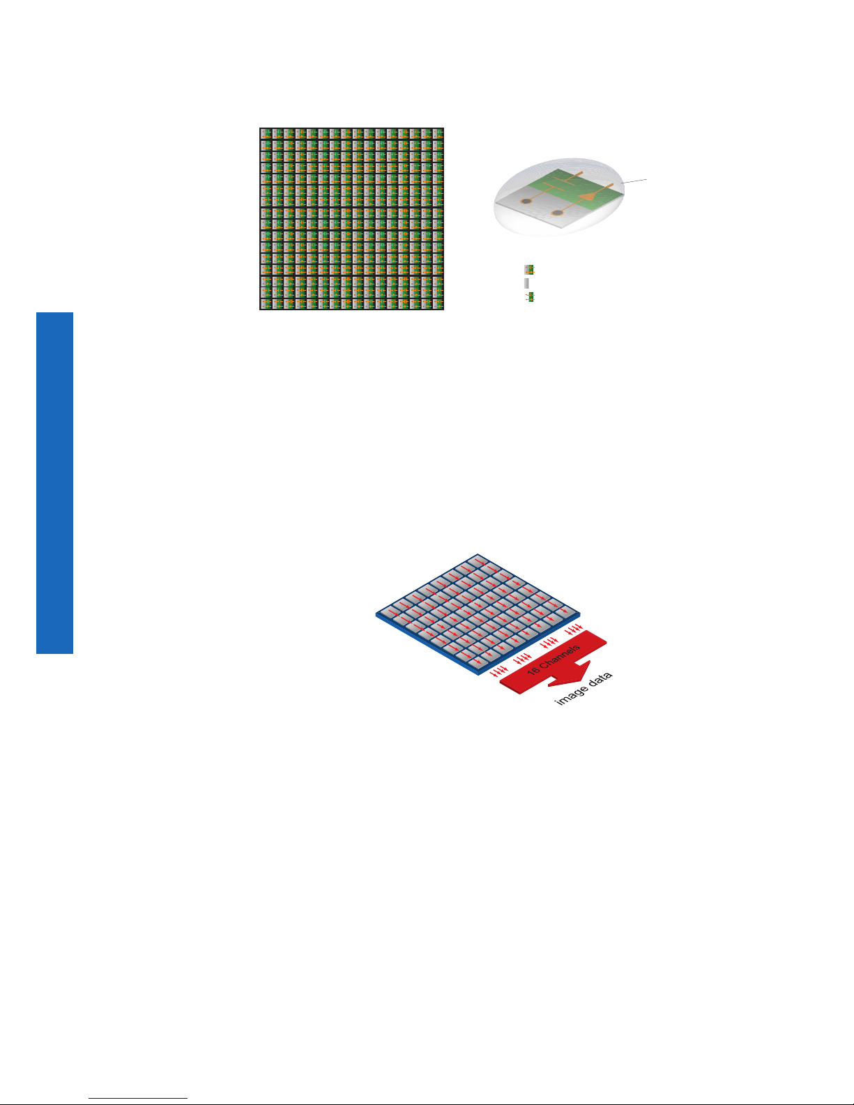
8.1.3 Digitization Taps
The CMOSIS sensors are read out with 16 channels in parallel.
Figure5►
Structure of an imaging sensor with global
shutter
Figure6►
Digitization Tap of the
Baumer LXG cameras
with Visual Applets
Readout with 16 channel
Page 19

19
8.1.4 Field of View Position
The typical accuracy by assumption of the root mean square value is displayed in the
gures and the table below:
±
β
A'
A
A'
A
±Y
±X
±X
±Y
M
M
R
R
LXG-40M.P
A'
A
±Y
±X
±X
±Y
M
M
R
R
β
A'
A
LXG-120M.P / LXG-200M.P
Camera
Type
± x
M,typ
[mm]
± y
M,typ
[mm]
± x
R,typ
[mm]
± y
R,typ
[mm]
± β
typ
[°]
LXG-40M.P 0.09 0.09 0.1 0.1 0.4
LXG-120M.P 0.07 0.06 0.08 0.07 0.26
LXG-200M.P 0.08 0.08 0.09 0.08 0.27
◄Figure7
Sensor accuracy of
Baumer LXG cameras
with Visual Applets.
Page 20

20
8.2 Timings
Notice
Overlapped mode can be switched off with setting the readout mode to sequential shut-
ter instead of overlapped shutter.
The image acquisition consists of two separate, successively processed components.
Exposing the pixels on the photosensitive surface of the sensor is only the rst part of the
image acquisition. After completion of the rst step, the pixels are read out.
Thereby the exposure time (t
exposure
) can be adjusted by the user, however, the time need-
ed for the readout (t
readout
) is given by the particular sensor and image format.
Baumer cameras can be operated with two modes, the Free Running Mode and the
Trigger Mode.
The cameras can be operated non-overlapped1) or overlapped. Depending on the mode
used, and the combination of exposure and readout time:
Non-overlapped Operation Overlapped Operation
Here the time intervals are long enough
to process exposure and readout successively.
In this operation the exposure of a frame
(n+1) takes place during the readout of
frame (n).
Exposur
e
Readout
Exposur
e
Readout
8.2.1 Free Running Mode
In the "Free Running" mode the camera records images permanently and sends them to
the PC. In order to achieve an optimal (with regard to the adjusted exposure time t
exposure
and image format) the camera is operated overlapped.
In case of exposure times equal to / less than the readout time (t
exposure
≤ t
readout
), the maximum frame rate is provided for the image format used. For longer exposure times the
frame rate of the camera is reduced.
Exposur
e
Readout
Flas
h
t
exposure(n)
t
flash(n)
t
flashdelay
t
flash(n+1)
t
readout(n+1)
t
readout(n)
t
exposure(n+1)
t
ash
= t
exposure
1) Non-overlapped means the same as sequential.
Image parameters:
Offset
Gain
Mode
Partial Scan
Timings:
A - exposure time
frame (n) effective
B - image parameters
frame (n) effective
C - exposure time
frame (n+1) effective
D - image parameters
frame (n+1) effective
Page 21

21
8.2.2 Trigger Mode
After a specied external event (trigger) has occurred, image acquisition is started. Depending on the interval of triggers used, the camera operates non-overlapped or overlapped in this mode.
With regard to timings in the trigger mode, the following basic formulas need to be taken
into consideration:
Case Formula
t
exposure
< t
readout
(1) t
earliestpossibletrigger(n+1)
= t
readout(n)
- t
exposure(n+1)
(2) t
notready(n+1)
= t
exposure(n)
+ t
readout(n)
- t
exposure(n+1)
t
exposure
> t
readout
(3) t
earliestpossibletrigger(n+1)
= t
exposure(n)
(4) t
notready(n+1)
= t
exposure(n)
8.2.2.1 Overlapped Operation: t
exposure(n+2)
= t
exposure(n+1)
In overlapped operation attention should be paid to the time interval where the camera is
unable to process occuring trigger signals (t
notready
). This interval is situated between two
exposures. When this process time t
notready
has elapsed, the camera is able to react to
external events again.
After t
notready
has elapsed, the timing of (E) depends on the readout time of the current im-
age (t
readout(n)
) and exposure time of the next image (t
exposure(n+1)
). It can be determined by the
formulas mentioned above (no. 1 or 3, as is the case).
In case of identical exposure times, t
notready
remains the same from acquisition to acquisi-
tion.
Exposur
e
Readout
t
exposure(n)
t
readout(n+1)
t
readout(n)
t
exposure(n+1)
t
triggerdelay
t
min
Tr
igger
Flas
h
t
flash(n)
t
flashdelay
t
flash(n+1)
Tr
iggerReady
t
notready
Image parameters:
Offset
Gain
Mode
Partial Scan
Timings:
A - exposure time
frame (n) effective
B - image parameters
frame (n) effective
C - exposure time
frame (n+1) effective
D - image parameters
frame (n+1) effective
E - earliest possible trigger
Page 22

22
8.2.2.2 Overlapped Operation: t
exposure(n+2)
> t
exposure(n+1)
If the exposure time (t
exposure
) is increased from the current acquisition to the next acquisi-
tion, the time the camera is unable to process occuring trigger signals (t
notready
) is scaled
down.
This can be simulated with the formulas mentioned above (no. 2 or 4, as is the case).
Exposure
Readout
t
exposure(n)
t
readout(n+1)
t
readout(n)
t
exposure(n+1)
t
exposure(n+2)
t
triggerdelay
t
min
Trigger
Flas
h
t
flash(n)
t
flashdelay
t
flash(n+1)
TriggerReady
t
notready
Image parameters:
Offset
Gain
Mode
Partial Scan
Timings:
A - exposure time
frame (n) effective
B - image parameters
frame (n) effective
C - exposure time
frame (n+1) effective
D - image parameters
frame (n+1) effective
E - earliest possible trigger
Page 23

23
8.2.2.3 Overlapped Operation: t
exposure(n+2)
< t
exposure(n+1)
If the exposure time (t
exposure
) is decreased from the current acquisition to the next acquisi-
tion, the time the camera is unable to process occuring trigger signals (t
notready
) is scaled
up.
When decreasing the t
exposure
such, that t
notready
exceeds the pause between two incoming
trigger signals, the camera is unable to process this trigger and the acquisition of the im-
age will not start (the trigger will be skipped).
Exposur
e
Readout
t
exposure(n)
t
readout(n+1)
t
readout(n)
t
exposure(n+1)
t
exposure(n+2)
t
triggerdelay
t
min
Tr
igger
Flas
h
t
flash(n)
t
flashdelay
t
flash(n+1)
Tr
iggerReady
t
notready
Notice
From a certain frequency of the trigger signal, skipping triggers is unavoidable. In general, this frequency depends on the combination of exposure and readout times.
Image parameters:
Offset
Gain
Mode
Partial Scan
Timings:
A - exposure time
frame (n) effective
B - image parameters
frame (n) effective
C - exposure time
frame (n+1) effective
D - image parameters
frame (n+1) effective
E - earliest possible trigger
F - frame not started /
trigger skipped
Page 24

24
8.2.2.4 Non-overlapped Operation
If the frequency of the trigger signal is selected for long enough, so that the image acquisitions (t
exposure
+ t
readout
) run successively, the camera operates non-overlapped.
Exposure
Readout
t
exposure(n)
t
readout(n+1)
t
readout(n)
t
exposure(n+1)
t
triggerdelay
t
min
Trigger
Flas
h
t
flash(n)
t
flashdelay
t
flash(n+1)
TriggerReady
t
notready
Image parameters:
Offset
Gain
Mode
Partial Scan
Timings:
A - exposure time
frame (n) effective
B - image parameters
frame (n) effective
C - exposure time
frame (n+1) effective
D - image parameters
frame (n+1) effective
E - earliest possible trigger
Page 25

25
9. Software
9.1 Baumer GAPI SDK
Baumer GAPI stands for Baumer “Generic Application Programming Interface”. With this
API Baumer provides an interface for optimal integration and control of Baumer cameras.
This software interface allows changing to other camera models.
It provides interfaces to several programming languages, such as C, C++ and the .NET™
Framework on Windows®, as well as Mono on Linux® operating systems, which offers the
use of other languages, such as e.g. C# or VB.NET.
For LXG cameras with Visual Applets Baumer GAPI SDK v 2.3 SP1 and higher is re-
quired.
9.2 3rd Party Software
Strict compliance with the GenICam™ standard allows Baumer to offer the use of 3rd
Party Software for operation with cameras.
You can nd a current listing of 3rd Party Software, which was tested successfully in combination with Baumer cameras, at http://www.baumer.com/?id=2851
Page 26

26
10. Camera Functionalities
10.1 Image Acquisition
10.1.1 Image Format
The cameras support the native resolution of the sensor.
In ROI mode the resolution (horizontal and vertical dimensions in pixels) can be adjusted.
Binning and Decimation are not available but can be implemented within Visual Applets
if required.
Page 27

27
10.1.2 Pixel Format
On Baumer digital cameras the pixel format depends on the selected image format.
10.1.2.1 Pixel Formats on Baumer LXG - Cameras with Visual Applets
Camera Type
Mono10
Mono10Packed
Mono12
Mono12Packed
LXG-40M.P ■ ■ □ □
LXG-120M.P □ □ ■ ■
LXG-200M.P □ □ ■ ■
10.1.2.2 Denitions
Notice
Below is a general description of pixel formats. The table above shows, which camera
support which formats.
Bayer: Raw data format of color sensors.
Color lters are placed on these sensors in a checkerboard pattern, generally
in a 50% green, 25% red and 25% blue array.
Mono: Monochrome. The color range of mono images consists of shades of a single
color. In general, shades of gray or black-and-white are synonyms for monochrome.
◄Figure8
Sensor with Bayer
Pattern.
Page 28

28
RGB: Color model, in which all detectable colors are dened by three coordinates,
Red, Green and Blue.
Red
Gree
n
Blue
Black
White
The three coordinates are displayed within the buffer in the order R, G, B.
BGR: Here the color alignment mirrors RGB.
YUV: Color model, which is used in the PAL TV standard and in image compression.
In YUV, a high bandwidth luminance signal (Y: luma information) is transmitted
together with two color difference signals with low bandwidth (U and V: chroma
information). Thereby U represents the difference between blue and luminance
(U = B - Y), V is the difference between red and luminance (V = R - Y). The third
color, green, does not need to be transmitted, its value can be calculated from
the other three values.
YUV 4:4:4 Here each of the three components has the same sample rate.
Therefore there is no subsampling here.
YUV 4:2:2 The chroma components are sampled at half the sample rate.
This reduces the necessary bandwidth to two-thirds (in relation to
4:4:4) and causes no, or low visual differences.
YUV 4:1:1 Here the chroma components are sampled at a quarter of the
sample rate.This decreases the necessary bandwith by half (in
relation to 4:4:4).
Pixel depth: In general, pixel depth denes the number of possible different values for
each color channel. Mostly this will be 8 bit, which means 28 different "colors".
For RGB or BGR these 8 bits per channel equal 24 bits overall.
8 bit:
Byte 1 Byte 2 Byte 3
10 bit:
Byte 1 Byte 2
unused bits
12 bit:
Byte 1 Byte 2
unused bits
Figure9►
RBG color space displayed as color tube.
Figure10►
Bit string of Mono 8 bit
and RGB 8 bit.
Figure12►
Spreading of Mono 12
bit over two bytes.
Figure11►
Spreading of Mono 10
bit over 2 bytes.
Page 29

29
10.1.3 Exposure Time
On exposure of the sensor, the inclination of photons produces a charge separation on
the semiconductors of the pixels. This results in a voltage difference, which is used for
signal extraction.
Light
Photon
Pixel
Charge Carrier
The signal strength is inuenced by the incoming amount of photons. It can be increased
by increasing the exposure time (t
exposure
).
On Baumer LXG cameras with Visual Applets, the exposure time can be set within the
following ranges (step size 1μsec):
Camera Type t
exposure
min t
exposure
max
LXG-40M.P 57 μsec 1 sec
LXG-120M.P 55 μsec 1 sec
LXG-200M.P 44 μsec 1 sec
Notice
The exposure time can be programmed or controlled via trigger width.
However, the sensor needs additional time for the sampling operation during which the
sensor is still light sensitive. As a consequence the real minimum exposure time is the
respective t
exposure
min longer.
10.1.4 PRNU / DSNU Correction (FPN - Fixed Pattern Noise)
CMOS sensors exhibit nonuniformities that are often called xed pattern noise (FPN).
However it is no noise but a xed variation from pixel to pixel that can be corrected. The
advantage of using this correction is a more homogeneous picture which may simplify the
image analysis. Variations from pixel to pixel of the dark signal are called dark signal nonuniformity (DSNU) whereas photo response nonuniformity (PRNU) describes variations
of the sensitivity. DNSU is corrected via an offset while PRNU is corrected by a factor.
The correction is based on columns. It is important that the correction values are comput-
ed for the used sensor readout conguration. During camera production this is derived for
the factory defaults. If other settings are used (e.g. different number of readout channels)
using this correction with the default data set may degrade the image quality. In this case
the user may derive a specic data set for the used setup.
PRNU / DSNU Correction Off PRNU / DSNU Correction On
◄Figure13
Incidence of light
causes charge separation on the semiconductors of the sensor.
Page 30

30
10.1.5 HDR
Beside the standard linear response the sensor supports a special high dynamic range
mode (HDR) called piecewise linear response. With this mode illuminated pixels that
reach a certain programmable voltage level will be clipped. Darker pixels that do not reach
this threshold remain unchanged. The clipping can be adjusted two times within a single
exposure by conguring the respective time slices and clipping voltage levels. See the
gure below for details.
In this mode, the values for t
Expo0
, t
Expo1
, Pot0 and Pot1can be edited.
The value for t
Expo2
will be calculated automatically in the camera. (t
Expo2
= t
exposure
- t
Expo0
-
t
Expo1
)
HDR Off HDR On
L
ow Illumination
High
Illumination
Pot
0
Pot
1
Pot
2
t
Expo0
t
Expo1tExpo2
t
exposure
Sensor Output
Page 31

31
10.1.6 Region of Interest (ROI)
With this functions it is possible to predene a so-called Region of Interest (ROI) or Partial
Scan. The ROI is an area of pixels of the sensor. After image acquisition, only the information of these pixels is sent to the PC.
This functions is turned on, when only a region of the eld of view is of interest. It is
coupled to a reduction in resolution and increases the frame rate.
The ROI is specied by following values:
▪ Region Selector Region 0
▪ Region Mode On/Off
▪ Offset X - x-coordinate of the rst relevant pixel
▪ Offset Y - y-coordinate of the rst relevant pixel
▪ Width - horizontal size of the ROI
▪ Height - vertical size of the ROI
Notice
The values of the Offset X and Size X must be a multible of 32!
The step size in Y direction is 1 pixel at monochrome cameras and 2 pixel at color cameras.
Notice
If defect pixels should exist in the rst (mono cameras) or in the rst two (color
cameras) rows or columns of a ROI, these cannot be corrected with the defect
pixel correction. In this case you need to move or increase the ROI by a few
pixels.
The coordinates of defect pixels can be read out with the Camera Explorer
(Category: Control LUT).
Start ROI
End ROI
◄Figure14
Parameters of the ROI.
Page 32

32
10.1.6.1 ROI Readout (Region 0)
For the sensor readout time of the ROI, the horizontal subdivision of the sensor is unimportant – only the vertical subdivision is of importance.
Notice
The activation of ROI turns off all Multi-ROIs.
Start ROI
End ROI
The readout is line based, which means always a complete line of pixels needs to be read
out and afterwards the irrelevant information is discarded.
Start ROI
End ROI
Figure15►
ROI: Readout
Page 33

33
10.2 Analog Controls
10.2.1 Offset / Black Level
On Baumer LXG cameras with Visual Applets the offset (or black level) is adjustable .
Camera Type 1 step = 4 LSB
Relating to [bit]
LXG-40M.P 0 ... 63 LSB | 10 bit
LXG-120M.P 0 .. 255 LSB | 12 Bit
LXG-200M.P 0 .. 255 LSB | 12 Bit
10.2.2 Gain
In industrial environments motion blur is unacceptable. Due to this fact exposure times
are limited. However, this causes low output signals from the camera and results in dark
images. To solve this issue, the signals can be amplied by user within the camera. This
gain is adjustable from 0 to 12 db.
Notice
Increasing the gain factor causes an increase of image noise and leads to missing
codes at Mono12, if the gain factor > 1.0.
10.3 Defect Pixel Correction
Notice
If defect pixels should exist in the rst (mono cameras) or in the rst two (color
cameras) rows or columns of a ROI, these cannot be corrected with the defect
pixel correction. In this case you need to move or increase the ROI by a few
pixels.
The coordinates of defect pixels can be read out with the Camera Explorer
(Category: Control LUT).
10.3.1 General information
A certain probability for abnormal pixels - the so-called defect pixels - applies to the sensors of all manufacturers. The charge quantity on these pixels is not linear-dependent on
the exposure time.
The occurrence of these defect pixels is unavoidable and intrinsic to the manufacturing
and aging process of the sensors.
The operation of the camera is not affected by these pixels. They only appear as brighter
(warm pixel) or darker (cold pixel) spot in the recorded image.
Warm Pixel
Cold Pixel
Charge quantity
„Normal Pixel“
Charge quantity
„Cold Pixel“
Charge quantity
„Warm Pixel“
◄Figure16
Distinction of "hot" and
"cold" pixels within the
recorded image.
◄Figure17
Charge quantity of "hot" and
"cold" pixels compared with
"normal" pixels.
Page 34

34
10.3.2 Correction Algorithm
On Baumer LXG cameras with Visual Applets the problem of defect pixels is solved as
follows:
▪ Possible defect pixels are identied during the production process of the camera.
▪ The coordinates of these pixels are stored in the factory settings of the camera.
Once the sensor readout is completed, correction takes place:
▪ Before any other processing, the values of the neighboring pixels with the same
color on the left and the right side of the defect pixel, will be read out
▪ Then the average value of these pixels is determined
▪ Finally, the value of the defect pixel is substituted by the previously determined
average value
This works horizontally and vertically. With this approach whole defect rows and defect
columns can be corrected.
Defect Pixel Average Value Corrected Pixel
10.3.3 DefectPixelList
As stated previously, this list is determined within the production process of Baumer cameras and stored in the factory settings. This list is editable.
Figure18►
Schematic diagram of
the Baumer pixel
correction.
Page 35

35
10.4 Sequencer
10.4.1 General Information
A sequencer is used for the automated control of series of images using different sets of
parameters.
m
o
z
n
A
n
B
n
C
n
x-1
A
B
C
The gure above displays the fundamental structure of the sequencer module.
The loop counter (m) represents the number of sequence repetitions.
The repeat counter (n) is used to control the amount of images taken with the respective
sets of parameters. For each set there is a separate n.
The start of the sequencer can be realized directly (free running) or via an external event
(trigger). The source of the external event (trigger source) must be determined before.
The additional frame counter (z) is used to create a half-automated sequencer. It is absolutely independent from the other three counters, and used to determine the number of
frames per external trigger event.
The following timeline displays the temporal course of a sequence with:
▪ n = (A=5), (B=3), (C=2) repetitions per set of parameters
▪ o = 3 sets of parameters (A,B and C)
▪ m = 1 sequence and
▪ z = 2 frames per trigger
t
n = 1
n = 2
n = 3
n = 4
n = 5
n = 1
n = 2
n = 3
n = 1n = 2
ABC
z = 2z = 2z = 2z = 2z = 2
◄Figure19
Flow chart of
sequencer.
m - number of loop
passes
n - number of set
repetitions
o - number of
sets of parameters
z - number of frames
per trigger
Sequencer Parameter:
The mentioned sets of
parameter include the
following:
▪ Exposure time
▪ Gain factor
▪ Output line value
▪ Origin of ROI (Offset X, Y
)
◄Figure20
Timeline for a single
sequence
Page 36

36
10.4.2 Baumer Optronic Sequencer in Camera xml-le
The Baumer Optronic seqencer is described in the category
“BOSequencer”
by the follow-
ing features:
Static Sequencer Features
These values are valid for all sets.
BoSequencerEnable
Enable / Disable
BoSequencerFramesPerTrigger
Number of frames per trigger (z)
BoSequencerIsRunning
Check whether the sequencer is running
BoSequencerLoops
Number of sequences (m)
BoSequencerMode
Running mode of Sequencer
BoSequencerSetNumberOfSets
Number of sets - 1
BoSequencerStart
Start / Stop
BoSequencerSetActive
Returns the index of the active set of the
running sequencer.
Set-specicFeatures
These values can be set individually for each set.
BoSequencerExposure
Parameter exposure
BoSequencerGain
Parameter gain
BoSequencerOffsetX
ROI Offset X
BoSequencerOffsetY
ROI Offset Y
BoSequencerIOSelector
Selected output lines
BoSequencerIOStatus
Status of all Sequencer outputs
BoSequencerSetRepeats
Number of repetitions (n)
BoSequencerSetSelector
Congure set of parameters
10.4.3 Examples
10.4.3.1 Sequencer without Machine Cycle
Sequencer
Start
A
A
B
B
C
C
The gure above shows an example for a fully automated sequencer with three sets of
parameters (A, B and C). Here the repeat counter (n) is set for (A=5), (B=3), (C=2) and
the loop counter (m) has a value of 2.
When the sequencer is started, with or without an external event, the camera will record
the pictures using the sets of parameters A, B and C (which constitutes a sequence).
After that, the sequence is started once again, followed by a stop of the sequencer - in this
case the parameters are maintained.
Figure21►
Example for a fully automated sequencer.
Page 37

37
10.4.3.2 Sequencer Controlled by Machine Steps (trigger)
A
A
B
B
C
C
Trigger
Sequencer
Start
The gure above shows an example for a half-automated sequencer with three sets of
parameters (A,B and C) from the previous example. The frame counter (z) is set to 2. This
means the camera records two pictures after an incoming trigger signal.
10.4.4 Capability Characteristics of Baumer GAPI Sequencer Module
▪ up to 128 sets of parameters
▪ up to 2 billion loop passes
▪ up to 2 billion repetitions of sets of parameters
▪ up to 2 billion images per trigger event
▪ free running mode without initial trigger
◄Figure22
Example for a half-auto-
mated sequencer.
Page 38

38
10.4.5 Double Shutter
This feature offers the possibility of capturing two images in a very short interval. Depend-
ing on the application, this is performed in conjunction with a ash unit. Thereby the rst
exposure time (t
exposure
) is arbitrary and accompanied by the rst ash. The second expo-
sure time must be equal to, or longer than the readout time (t
readout
) of the sensor. Thus the
pixels of the sensor are recepitve again shortly after the rst exposure. In order to realize
the second short exposure time without an overrun of the sensor, a second short ash
must be employed, and any subsequent extraneous light prevented.
Tr
igger
Prevent Light
Exposur
e
Readout
Flas
h
On Baumer LXG cameras with Visual Applets this feature is realized within the sequencer.
In order to generate this sequence, the sequencer must be congured as follows:
Parameter Setting:
Sequencer Run Mode Once by Trigger
Sets of parameters (o) 2
Loops (m) 1
Repeats (n) 1
Frames Per Trigger (z) 2
Figure23►
Example of a double
shutter.
Page 39

39
10.5 Process Interface
10.5.1 Digital I/O
All Baumer LXG cameras with Visual Applets are equipped with one input line and three
output lines.
10.5.1.1 I/O Circuits
Notice
Low Active: At this wiring, only one consumer can be connected. When all Output pins
(1, 2, 3) connected to I/O_GND, then current ows through the resistor as soon as one
Output is switched. If only one output connected to I/O_GND, then this one is only usable.
The other two Outputs are not usable and may not be connected (e.g. I/O Power VCC)!
Output high active Output low active Input
Camera Customer Device
IO Power V
CC
U
ext
Pin
R
L
I
OUT
IO GND
Out (n)
Pin
Camera Customer Device
IO Power V
CC
R
L
I
OUT
IO GND
Out
U
ext
Pin (Out1, 2, 3)
Out1 or Out2
or Out3
CameraCustomer Device
IO GND
DRV
IN1 Pin
IN_GND Pin
10.5.1.2 UserDenableInputs
The wiring of the input connector is left to the user.
Sole exception is the compliance with predetermined high and low levels (0 .. 4,5V low,
11 .. 30V high).
The dened signals will have no direct effect, but can be analyzed and processed on the
software side and used for controlling the camera.
The employment of a so called "IO matrix" offers the possibility of selecting the signal and
the state to be processed.
On the software side the input signals are named "Line0".
(Input) Line0
state high
state low
Line0
IO Matrix
state selection
(software side)
◄Figure24
IO matrix of the
Baumer LXG cameras
with Visual Applets on
input side.
Page 40

40
10.5.1.3 CongurableOutputs
With this feature, Baumer offers the possibility of wiring the output connectors to internal
signals, which are controlled on the software side.
Hereby on Baumer LXG cameras with Visual Applets 17 signal sources – subdivided into
three categories – can be applied to the output connectors.
The rst category of output signals represents a loop through of signals on the input side,
such as:
Signal Name Explanation
Line0 Signal of input "Line0" is loopthroughed to this ouput
Line1 Signal of input "Line1" is loopthroughed to this ouput
Line2 Signal of input "Line2" iys loopthroughed to this ouput
Within the second category you will nd signals that are created on camera side:
Signal Name Explanation
FrameActive The camera processes a Frame consisting of exposure
and readout
TriggerReady Camera is able to process an incoming trigger signal
TriggerOverlapped The camera operates in overlapped mode
TriggerSkipped Camera rejected an incoming trigger signal
ExposureActive Sensor exposure in progress
TransferActive Image transfer via hardware interface in progress
ExposureEnlarged This output marks the period of enlarged exposure time
Beside the 10 signals mentioned above, each output can be wired to a user-dened
signal ("UserOutput0", "UserOutput1", "UserOutput2", "SequencerOut 0...2" or disabled
("OFF").
(Output) Line 1
state high
state low
(Output) Line 2
state high
state low
(Output) Line 3
state high
state low
IO Matrix
state selection
(software side)
signal selection
(software side)
O
Line0
Line1
Line2
FrameActive
TriggerReady
TriggerOverlapped
TriggerSkipped
ExposureActive
TransferActive
ExposureEnlarged
UserOutput0
UserOutput1
UserOutput2
Timer1Active
Timer2Active
Timer3Active
SequencerOutput0
SequencerOutput1
SequencerOutput2
User defined Signals Internal Signals
Loopthroughed
Signals
Figure25►
IO matrix of the
Baumer LXG cameras
with Visual Applets on
output side.
Page 41

41
10.6 Trigger Input / Trigger Delay
Trigger signals are used to synchronize the camera exposure and a machine cycle or, in
case of a software trigger, to take images at predened time intervals.
Different trigger sources can be used here:
Line0 Actioncommand
Line1 Off
Line2
SW-Trigger
Possible settings of the Trigger Delay: :
Delay 0-2 sec
Number of tracked Triggers 512
Step 1 µsec
There are three types of modes. The timing diagrams for the three types you can see
below.
Normal Trigger with adjusted Exposure
Trigger (valid)
Exposure
Readout
Time
A
B
C
Pulse Width controlled Exposure
Trigger (valid)
Exposure
Readout
Time
B
C
Figure26▲
Trigger signal, valid for
Baumer cameras.
high
low
U
t0
4.5V
11V
30V
Camera in trigger
mode:
A - Trigger delay
B - Exposure time
C - Readout time
Page 42

42
10.6.1 Trigger Source
p
h
o
t
o
e
l
e
c
t
r
i
c
s
e
n
s
o
r
t
r
i
g
g
e
r
s
i
g
n
a
l
p
r
o
g
r
a
m
m
a
b
l
e
l
o
g
i
c
c
o
n
t
r
o
l
l
e
r
o
t
h
e
r
s
s
o
f
t
w
a
r
e
t
r
i
g
g
e
r
H
a
r
d
w
a
r
e
t
r
i
g
g
e
r
Each trigger source has to be activated separately. When the trigger mode is activated,
the hardware trigger is activated by default.
Figure27►
Examples of possible
trigger sources.
Page 43

43
10.6.2 Debouncer
The basic idea behind this feature was to seperate interfering signals (short peaks) from
valid square wave signals, which can be important in industrial environments. Debouncing
means that invalid signals are ltered out, and signals lasting longer than a user-dened
testing time t
DebounceHigh
will be recognized, and routed to the camera to induce a trigger.
In order to detect the end of a valid signal and lter out possible jitters within the signal, a
second testing time t
DebounceLow
was introduced. This timing is also adjustable by the user.
If the signal value falls to state low and does not rise within t
DebounceLow
, this is recognized
as end of the signal.
The debouncing times t
DebounceHigh
and t
DebounceLow
are adjustable from 0 to 5 msec in steps
of 1 μsec.
This feature is disabled by default.
low
high
U
t0
4.5V
11V
30V
low
high
U
t0
4.5V
11V
30V
t
∆t
1
∆tx - high time of the signal
t
DebounceHigh
- user-defined debouncer delay for state high
t
DebounceLow
- user-defined debouncer delay for state low
t
DebounceHigh
∆t
2
∆t
3
∆t4∆t
5
∆t
6
t
DebounceLow
Incoming signals
(valid and invalid)
Debouncer
Filtered signal
10.6.3 Flash Signal
On Baumer cameras, this feature is realized by the internal signal "ExposureActive",
which can be wired to one of the digital outputs.
Debouncer:
Please note that the edges
of valid trigger signals are
shifted by t
DebounceHigh
and
t
DebounceLow
!
Depending on these
two timings, the trigger
signal might be temporally
stretched or compressed.
◄Figure28
Principle of the Baumer
debouncer.
Page 44

44
10.6.4 Timer
Timers were introduced for advanced control of internal camera signals.
On Baumer LXG cameras with Visual Applets the timer conguration includes four components:
Setting Description
Timeselector There are three timers. Own settings for each timer can be
made . (Timer1, Timer2, Timer3)
TimerTriggerSource This feature provides a source selection for each timer.
TimerTriggerActivation This feature selects that part of the trigger signal (edges or
states) that activates the timer.
TimerDelay This feature represents the interval between incoming trig-
ger signal and the start of the timer.
(0 μsec .. 2 sec, step: 1 μsec)
TimerDuration By this feature the activation time of the timer is adjustable.
(10 μsec .. 2 sec, step: 1 μsec)
Different Timer sources can be used:
Input Line0 Frame Start
SW-Trigger Frame End
ActionCommandTrigger TriggerSkipped
Exposure Start
Exposure End
For example the using of a timer allows you to control the ash signal in that way, that the
illumination does not start synchronized to the sensor exposure but a predened interval
earlier.
For this example you must set the following conditions:
Setting Value
TriggerSource InputLine0
TimerTriggerSource InputLine0
Outputline1 (Source) Timer1Active
TimerTriggerActivation Falling Edge
Trigger Polarity Falling Edge
Exposure
Timer
t
exposure
t
triggerdelay
InputLine0
t
TimerDuration
t
TimerDelay
Page 45

45
10.7 User Sets
Notice
The Visual Applet design parameters are not stored in the user sets.
Three user sets (1-3) are available for the Baumer LXG cameras with Visual Applets. The
user sets can contain the following information:
Parameter
ChunkModeActive Events
ChunkEnable AcquisitionFrameRateEnable
DeviceTapGeometry AcquisitionFrameRate
DeviceClockFrequency PixelFormat
HDREnable BlackLevel
BlackReferenceCorrectionEnable Gain
FixedPatternNoiseCorrection TestPattern
SensorEffectCorrection ReverseX
ReadoutMode ReverseY
BoSequencerEnable LineMode
DefectPixelCorrection LineStatus
ExposureTime LineInverter
TriggerMode LineSource
TriggerWidth TimerDuration
TriggerSource TimerDelay
TriggerDelay TimerTriggerSource
PacketDelay TimerTriggerActivation
TransmissionDelay
ActionGroupKey
ActionGroupMask
These user sets are stored within the camera and and cannot be saved outside the device.
By employing a so-called "user set default selector", one of the three possible user sets
can be selected as default, which means, the camera starts up with these adjusted pa-
rameters.
10.8 Factory Settings
The factory settings are stored in an additional parametrization set which is used by default. This settings are not editable.
Page 46

46
11. Interface Functionalities
11.1 Device Information
This Gigabit Ethernet-specic information on the device is part of the Discovery-Acknowl-
edge of the camera.
Included information:
▪ MAC address
▪ Current IP conguration (persistent IP / DHCP / LLA)
▪ Current IP parameters (IP address, subnet mask, gateway)
▪ Manufacturer's name
▪ Manufacturer-specic information
▪ Device version
▪ Serial number
▪ User-dened name (user programmable string)
At the beginning of a frame will transmitted a Leader and at the end will transmitted a
Trailer.
Figure29►
Transmission of data
packets
Page 47

47
11.2 Baumer Image Info Header (Chunk Data)
The Baumer Chunk are data, which are generated by the camera.
These data include different settings for the respective image. Baumer GAPI can read this
settings. Third Party Software, which supports the Chunk mode, can read the settings in
the table below.
This settings may be for example (not completely):
Feature Description
ChunkOffsetX Horizontal offset from the origin to the area of interest (in
pixels).
ChunkOffsetY Vertical offset from the origin to the area of interest (in pix-
els).
ChunkWidth Returns the Width of the image included in the payload.
ChunkHeight Returns the Height of the image included in the payload.
ChunkPixelFormat Returns the PixelFormat of the image included in the pay-
load.
ChunkExposureTime Returns the exposure time used to capture the image.
ChunkBlackLevelSelector Selects which Black Level to retrieve data from.
ChunkBlackLevel Returns the black level used to capture the image included
in the payload.
ChunkFrameID Returns the unique Identier of the frame (or image) includ-
ed in the payload.
There are three chunk modes:
Image Data
Only the image data are transferred, no chunk data.
Page 48

48
Chunk Data
Only the chunk is transferred, no image data.
Extented Chunk Data
Chunk data and image data are transferred. The chunk data are included in the last data
packet.
11.3 Packet Size and Maximum Transmission Unit (MTU)
Network packets can be of different sizes. The size depends on the network components
employed. When using GigE Vision®- compliant devices, it is generally recommended
to use larger packets. On the one hand the overhead per packet is smaller, on the other
hand larger packets cause less CPU load.
The packet size of UDP packets can differ from 576 Bytes up to the MTU.
The MTU describes the maximal packet size which can be handled by all network com-
ponents involved.
In principle modern network hardware supports a packet size of 1518 Byte, which is specied in the network standard. However, so-called "Jumbo frames" are on the advance as
Gigabit Ethernet continues to spread. "Jumbo frames" merely characterizes a packet size
exceeding 1500 Bytes.
Baumer LXG cameras with Visual Applets can handle a MTU of up to 16384 Bytes.
Page 49

49
11.4 "Inter Packet Gap" (IPG)
To achieve optimal results in image transfer, several Ethernet-specic factors need to be
considered when using Baumer LXG cameras with Visual Applets.
Upon starting the image transfer of a camera, the data packets are transferred at maximum transfer speed (1 Gbit/sec). In accordance with the network standard, Baumer employs a minimal separation of 12 Bytes between two packets. This separation is called
"Inter Packet Gap" (IPG). In addition to the minimal PD, the GigE Vision® standard stipulates that the PD be scalable (user-dened).
11.4.1 Example 1: Multi Camera Operation – Minimal IPG
Setting the IPG to minimum means every image is transfered at maximum speed. Even
by using a frame rate of 1 fps this results in full load on the network. Such "bursts" can
lead to an overload of several network components and a loss of packets. This can occur,
especially when using several cameras.
In the case of two cameras sending images at the same time, this would theoretically occur at a transfer rate of 2 Gbits/sec. The switch has to buffer this data and transfer it at a
speed of 1 Gbit/sec afterwards. Depending on the internal buffer of the switch, this oper-
ates without any problems up to n cameras (n ≥ 1). More cameras would lead to a loss of
packets. These lost packets can however be saved by employing an appropriate resend
mechanism, but this leads to additional load on the network components.
◄Figure30
Packet Delay (PD) between the packets
▲Figure31
Operation of two cameras employing a Gigabit
Ethernet switch.
Data processing within
the switch is displayed
in the next two gures.
◄Figure32
Operation of two cameras employing a minimal
inter packet gap (IPG).
Page 50

50
11.4.2 Example 2: Multi Camera Operation – Optimal IPG
A better method is to increase the IPG to a size of
optimal IPG = packet size + 2 × minimal IPG
In this way both data packets can be transferred successively (zipper principle), and the
switch does not need to buffer the packets.
Figure33►
Operation of two cameras employing an optimal
inter packet gap (IPG).
Max. IPG:
On the Gigabit Ethernet
the max. IPG and the data
packet must not exceed 1
Gbit. Otherwise data packets can be lost.
Page 51

51
11.5 Frame Delay
Another approach for packet sorting in multi-camera operation is the so-called Frame De-
lay, which was introduced to Baumer Gigabit Ethernet cameras in hardware release 2.1.
Due to the fact, that the currently recorded image is stored within the camera and its
transmission starts with a predened delay, complete images can be transmitted to the
PC at once.
The following gure should serve as an example:
Due to process-related circumstances, the image acquisitions of all cameras end at the
same time. Now the cameras are not trying to transmit their images simultaniously, but –
according to the specied transmission delays – subsequently. Thereby the rst camera
starts the transmission immediately – with a transmission delay "0".
11.5.1 Time Saving in Multi-Camera Operation
As previously stated, the Frame delay feature was especially designed for multi-camera
operation with employment of different camera models. Just here an signicant acceleration of the image transmission can be achieved:
For the above mentioned example, the employment of the transmission delay feature re-
sults in a time saving – compared to the approach of using the inter paket gap – of approx.
45% (applied to the transmission of all three images).
◄Figure34
Principle of the Frame
delay.
◄Figure35
Comparison of frame
delay and inter packet
gap, employed for a
multi-camera system
with different camera
models.
Page 52

52
11.5.2 CongurationExample
For the three used cameras the following data are known:
Camera
Model
Sensor
Resolution
[Pixel]
Pixel Format
(Pixel Depth)
[bit]
Data
Volume
[bit]
Readout
Time
[msec]
Exposure
Time
[msec]
Transfer
Time
[msec]
LXG-200M.P 5120 x 3840 8 157286400 30.768 6 ≈ 73.24
LXG-200M.P 5120 x 3840 8 157286400 30.768 6 ≈ 73.24
LXG-200M.P 5120 x 3840 8 157286400 30.768 6 ≈ 73.24
▪ The sensor resolution and the readout time (t
readout
) can be found in the respective
Technical Data Sheet (TDS). For the example a full frame resolution is used.
▪ The exposure time (t
exposure
) is manually set to 6 msec.
▪ The resulting data volume is calculated as follows:
Resulting Data Volume = horizontal Pixels × vertical Pixels × Pixel Depth
All the cameras are triggered simultaniously.
The transmission delay is realized as a counter, that is started immediately after the sensor readout is started.
Camera 1
(SXG10)
Trigger
Camera 2
(SXG20)
Camera 3
(SXG80)
t
exposure(Camera 1)
t
exposure(Camera 2)
t
exposure(Camera 3)
t
readout(Camera 3)
t
transferGigE(Camera 3)
t
readout(Camera 2)
t
transferGigE(Camera 2)
t
readout(Camera 1)
t
transfer(Camera 1)*
TransmissionDelay
Camera 2
TransmissionDelay
Camera 3
In general, the transmission delay is calculated as:
Timings:
A - exposure start for all
cameras
B - all cameras ready for
transmission
C - transmission start
camera 2
D - transmission start
camera 3
Figure36►
Timing diagram for the
transmission delay of
the three employed
cameras, using even
exposure times.
Page 53

53
∑
≥
−
+−+=
n
3n
)1nCamera(gEtransferGi)nCamera(osureexp)1Camera(readout)1Camera(osureexp)nCamera(onDelayTransmissi
ttttt
Therewith for the example, the transmission delays of camera 2 and 3 are calculated as
follows:
t
TransmissionDelay(Camera 2)
= t
exposure(Camera 1)
+ t
readout(Camera 1)
- t
exposure(Camera 2)
t
TransmissionDelay(Camera 3)
= t
exposure(Camera 1)
+ t
readout(Camera 1)
- t
exposure(Camera 3)
+ t
transferGige(Camera 2)
Solving this equations leads to:
t
TransmissionDelay(Camera 2)
= 6 msec + 30.768 msec - 6 msec
= 30.768 msec
= 30768000 ticks
t
TransmissionDelay(Camera 3)
= 6 msec + 30.768 msec - 6 msec + 73.27 msec
= 104.038 msec
= 10403800 ticks
Notice
In Baumer GAPI the delay is specied in ticks. How do convert microseconds into
ticks?
1 tick = 1 ns
1 msec = 1000000 ns
1 tick = 0.000001 msec
ticks= t
TransmissionDelay
[msec] / 0.000001 = t
TransmissionDelay
[ticks]
Page 54

54
11.6 Multicast
Multicasting offers the possibility to send data packets to more than one destination address – without multiplying bandwidth between camera and Multicast device (e.g. Router
or Switch).
The data is sent out to an intelligent network node, an IGMP (Internet Group Management
Protocol) capable Switch or Router and distributed to the receiver group with the specic
address range.
In the example on the gure below, multicast is used to process image and message data
separately on two differents PC's.
Multicast Addresses:
For multicasting Baumer
suggests an adress
range from 232.0.1.0 to
232.255.255.255.
Figure37►
Principle of Multicast
Page 55

55
11.7 IPConguration
11.7.1 Persistent IP
A persistent IP adress is assigned permanently. Its validity is unlimited.
Notice
Please ensure a valid combination of IP address and subnet mask.
IP range: Subnet mask:
0.0.0.0 – 127.255.255.255 255.0.0.0
128.0.0.0 – 191.255.255.255 255.255.0.0
192.0.0.0 – 223.255.255.255 255.255.255.0
These combinations are not checked by Baumer GAPI, Baumer GAPI Viewer or camera
on the y. This check is performed when restarting the camera, in case of an invalid
IP - subnet combination the camera will start in LLA mode.
* This feature is disabled by default.
11.7.2 DHCP(DynamicHostCongurationProtocol)
The DHCP automates the assignment of network parameters such as IP addresses, subnet masks and gateways. This process takes up to 12 sec.
Once the device (client) is connected to a DHCP-enabled network, four steps are processed:
▪ DHCP Discovery
In order to nd a DHCP server, the client sends a so called DHCPDISCOVER broad-
cast to the network.
▪ DHCP Offer
After reception of this broadcast, the DHCP server will answer the request by a
unicast, known as DHCPOFFER. This message contains several items of information,
such as:
Information for the client
MAC address
offered IP address
Information on server
IP adress
subnet mask
duration of the lease
Internet Protocol:
On Baumer cameras IP v4
is employed.
Figure38▲
Connection pathway for
Baumer Gigabit Ethernet cameras:
The device connects
step by step via the
three described mechanisms.
DHCP:
Please pay attention to the
DHCP Lease Time.
◄Figure39
DHCP Discovery
(broadcast)
◄Figure40
DHCP offer (unicast)
Page 56

56
▪ DHCP Request
Once the client has received this DHCPOFFER, the transaction needs to be con-
rmed. For this purpose the client sends a so called DHCPREQUEST broadcast to the
network. This message contains the IP address of the offering DHCP server and
informs all other possible DHCPservers that the client has obtained all the necessary
information, and there is therefore no need to issue IP information to the client.
▪ DHCP Acknowledgement
Once the DHCP server obtains the DHCPREQUEST, a unicast containing all neces-
sary information is sent to the client. This message is called DHCPACK.
According to this information, the client will congure its IP parameters and the pro-
cess is complete.
11.7.3 LLA
LLA (Link-Local Address) refers to a local IP range from 169.254.0.1 to 169.254.254.254
and is used for the automated assignment of an IP address to a device when no other
method for IP assignment is available.
The IP address is determined by the host, using a pseudo-random number generator,
which operates in the IP range mentioned above.
Once an address is chosen, this is sent together with an ARP (Address Resolution Pro-
tocol) query to the network to check if it already exists. Depending on the response, the
IP address will be assigned to the device (if not existing) or the process is repeated.
This method may take some time - the GigE Vision® standard stipulates that establishing
connection in the LLA should not take longer than 40 seconds, in the worst case it can
take up to several minutes.
11.7.4 Force IP
1)
Inadvertent faulty operation may result in connection errors between the PC and the camera.
In this case "Force IP" may be the last resort. The Force IP mechanism sends an IP address and a subnet mask to the MAC address of the camera. These settings are sent
without verication and are adapted immediately by the client. They remain valid until the
camera is de-energized.
1) In the GigE Vision® standard, this feature is dened as "Static IP".
Figure41►
DHCP Request
(broadcast)
Figure42►
DHCP Acknowledgement (unicast)
DHCP Lease Time:
The validity of DHCP IP
addresses is limited by the
lease time. When this time
is elapsed, the IP conguration needs to be redone.
This causes a connection
abort.
LLA:
Please ensure operation
of the PC within the same
subnet as the camera.
Page 57

57
11.8 Packet Resend
Due to the fact, that the GigE Vision® standard stipulates using a UDP – a stateless user
datagram protocol – for data transfer, a mechanism for saving the "lost" data needs to be
employed.
Here, a resend request is initiated if one or more packets are damaged during transfer
and – due to an incorrect checksum – rejected afterwards.
On this topic one must distinguish between three cases:
11.8.1 Normal Case
In the case of unproblematic data transfer, all packets are transferred in their correct order
from the camera to the PC. The probability of this happening is more then 99%.
11.8.2 Fault 1: Lost Packet within Data Stream
If one or more packets are lost within the data stream, this is detected by the fact, that
packet number n is not followed by packet number (n+1). In this case the application
sends a resend request (A). Following this request, the camera sends the next packet and
then resends (B) the lost packet.
In our example packet no. 3 is lost. This fault is detected on packet no. 4, and the resend request triggered. Then the camera sends packet no. 5, followed by resending
packet no. 3.
◄Figure43
Data stream without
damaged or lost packets.
◄Figure44
Resending lost packets
within the data stream.
Page 58

58
11.8.3 Fault 2: Lost Packet at the End of the Data Stream
In case of a fault at the end of the data stream, the application will wait for incoming
packets for a predened time. When this time has elapsed, the resend request is
triggered and the "lost" packets will be resent.
In our example, packets from no. 3 to no. 5 are lost. This fault is detected after the predened time has elapsed and the resend request (A) is triggered. The camera then resends packets no. 3 to no. 5 (B) to complete the image transfer.
11.8.4 Termination Conditions
The resend mechanism will continue until:
▪ all packets have reached the pc
▪ the maximum of resend repetitions is reached
▪ the resend timeout has occured or
▪ the camera returns an error.
Figure45►
Resending of lost packets at the end of the
data stream.
Page 59

59
11.9 Message Channel
The asynchronous message channel is described in the GigE Vision® standard and offers the possibility of event signaling. There is a timestamp (64 bits) for each announced
event, which contains the accurate time the event occurred. Each event can be activated
and deactivated separately.
EventMap LXG cameras with Visual Applets:
Bit Edge Event-ID XML-Event-Description
GigE Vision Standard Events
0x0007 PrimaryApplicationSwitch
Hardware-Events
0 rising 0x9000 Line0RisingEdge
1 falling 0x9001 Line0FallingEdge
2 rising 0x9002 Line1RisingEdge
3 falling 0x9003 Line1FallingEdge
4 rising 0x9004 Line2RisingEdge
5 falling 0x9005 Line2FallingEdge
6 rising 0x9006 Line3RisingEdge
7 falling 0x9007 Line3FallingEdge
12 rising 0x900C ExposureStart
13 rising 0x900D ExposureEnd
14 rising 0x900E FrameStart
15 rising 0x900F FrameEnd
16 rising 0x9010 TriggerReady
17 rising 0x9011 TriggerOverlapped
18 rising 0x9012 TriggerSkipped
20 rising 0x9014 Action1
Software-Events
0x9020 GigEVisionError
0x9021 EventLost
0x9022 EventDiscarded
0x9023 GigEVisionHeartbeatTimeOut
Page 60

60
11.10 Action Commands
The basic idea behind this feature was to achieve a simultaneous trigger for multiple
cameras.
Action Command Description
Action Command Trigger used to send a trigger to all connected
cameras.
Therefore a broadcast ethernet packet was implemented. This packet can be used to
induce a trigger as well as other actions.
Due to the fact that different network components feature different latencies and jitters,
the trigger over the Ethernet is not as synchronous as a hardware trigger. Nevertheless,
applications can deal with these jitters in switched networks, and therefore this is a comfortable method for synchronizing cameras with software additions.
The action command is sent as a broadcast. In addition it is possible to group cameras,
so that not all attached cameras respond to a broadcast action command.
Such an action command contains:
▪ a Device Key - for authorization of the action on this device
▪ a Group Key - for triggering actions on separated groups of devices
▪ a Group Mask - for extension of the range of separate device groups
11.10.1 Action Command Trigger
The gure below displays three cameras, which are triggered synchronously by a software application.
Another application of action command is that a secondary application or PC or one of the
attached cameras can actuate the trigger.
Figure46►
Triggering of multiple
cameras via trigger over
Ethernet (ToE).
Page 61

61
12. Start-Stop-Behaviour
12.1 Start / Stop Acquisition (Camera)
Once the image acquisition is started, three steps are processed within the camera:
▪ Determination of the current set of image parameters
▪ Exposure of the sensor
▪ Readout of the sensor.
Afterwards a repetition of this process takes place until the camera is stopped.
Stopping the acquisition means that the process mentioned above is aborted. If the stop
signal occurs within a readout, the current readout will be nished before stopping the
camera. If the stop signal arrives within an exposure, this will be aborted.
Special Case: Asynchronous Reset
The asynchronous reset represents a special case of stopping the current acquisition.
Thereby exposure is aborted immediately. Thus the current image is not read out and the
image is upcasted.
This feature was introduced to accelerate the changing of image parameters.
12.2 Start / Stop Interface
Without starting the interface, transmission of image data from the camera to the PC
will not proceed. If the image acquisition is started befor the interface is activated, the
recorded images are lost.
If the interface is stopped during a transmission, this is aborted immediately.
12.3 Pause / Resume Interface
Pausing while the interface is operational, results in an interim storage of the recorded
images within the internal buffer of the camera.
After resuming the interface, the buffered image data will be transferred to the PC.
12.4 Acquisition Modes
In general, three acquisition modes are available for LXG cameras with Visual Applets.
12.4.1 Free Running
Free running means the camera records images continuously without external events.
12.4.2 Trigger
The basic idea behind the trigger mode is the synchronization of cameras with machine
cycles. Trigger mode means that image recording is not continuous, but triggered by
external events.
12.4.3 Sequencer
A sequencer is used for the automated control of series of images, using different settings
for exposure time and gain.
Asynchronous Reset:
For further information on
the timings of this feature,
please see the respective
data sheets.
Page 62

62
13. Cleaning
Avoid cleaning if possible. To prevent dust, follow the instructions under Installation.
Notice
Perform the cleaning in a dust-free room with clean tools. Use localized ionized air ow
on to the glass during cleaning.
13.1 Sensor
Recommended Equipment
▪ Miroscope
▪ Air gun
▪ Single drop bottle with pure alcohol
▪ Swab
▪ Phillips screwdriver
Procedure
1. Make sure that the contamination is not on the sensor glass
(except LXG-40M.P) or the installed lens.
2. Uninstall the lens mount adapter ( LXG-40M.P). Uninstall the sensor glass
(except LXG-40M.P) using the phillips screw driver.
3. Blow away mobile contamination using the air gun.
4. Place the sensor under the microscope to determine the location of any
remaining contamination.
5. Clean the contamination on the sensor using one drop pure alcohol on a swab.
Wipe the swab from left to right (or conversely, but only in one direction). Do this
in an overlapping pattern, turning the swab after the rst wipe and with each
subsequent wipe. Avoid swiping back and forth with the same swab in order to
ensure that particles are removed and not transferred to a new location on the
sensor. Use several swabs for this procedure.
13.2 Cover glass
If you must clean it, use compressed air or a soft, lint free cloth dampened with a small
quantity of pure alcohol.
13.3 Housing
Caution!
volatile
solvents
Volatile solvents for cleaning.
Volatile solvents damage the surface of the camera.
Never use volatile solvents (benzine, thinner) for cleaning!
To clean the surface of the camera housing, use a soft, dry cloth. To remove persistent
stains, use a soft cloth dampened with a small quantity of neutral detergent, then wipe dry.
Page 63

63
14. Transport / Storage
Notice
Transport the camera only in the original packaging. When the camera is not installed,
then storage the camera in the original packaging.
Storage Environment
Storage temperature -10°C ... +70°C ( +14°F ... +158°F)
Storage Humidy 10% ... 90% non condensing
15. Disposal
Dispose of outdated products with electrical or electronic circuits, not in the
normal domestic waste, but rather according to your national law and the
directives 2002/96/EC and 2006/66/EC for recycling within the competent
collectors.
Through the proper disposal of obsolete equipment will help to save valuable resources and prevent possible adverse effects on human health and
the environment.
The return of the packaging to the material cycle helps conserve raw materials an reduces the production of waste. When no longer required, dispose
of the packaging materials in accordance with the local regulations in force.
Keep the original packaging during the warranty period in order to be able
to pack the device in the event of a warranty claim.
16. Warranty Information
Notice
There are no adjustable parts inside the camera!
In order to avoid the loss of warranty do not open the housing!
Notice
If it is obvious that the device is / was dismantled, reworked or repaired by other than
Baumer technicians, Baumer will not take any responsibility for the subsequent perfor-
mance and quality of the device!
Page 64

64
17. Conformity
Baumer LXG cameras with Visual Applets comply with:
▪ CE
▪ RoHS
17.1 CE
We declare, under our sole responsibility, that the previously described Baumer LXG
cameras with Visual Applets conform with the directives of the CE (electromagnetic compatibility (EMC) 2004/108EC).
18. Support
If you have any problems with the camera, then feel free to contact our support.
Worldwide
Baumer Optronic GmbH
Badstrasse 30
DE-01454 Radeberg, Germany
Tel: +49 (0)3528 4386 845
Mail: support.cameras@baumer.com
Website: www.baumer.com
Page 65

65
Page 66

Baumer Optronic GmbH
Badstrasse 30
DE-01454 Radeberg, Germany
Phone +49 (0)3528 4386 0 · Fax +49 (0)3528 4386 86
sales@baumeroptronic.com · www.baumer.com
Technical data has been fully checked, but accuracy of printed matter not guaranteed.
Subject to change without notice. Printed in Germany.
 Loading...