BAS 100B/W Instruction Manual

Download

Page 1

BAS 100B/W Version 2.3

March 2001

MF-9094 INSTRUCTION MANUAL

Electrochemical Workstation

Bioanalytical Systems, Inc

2701 Kent Avenue West Lafayette Indiana 47906

Page 2

MANUFACTURER’S NOTE

This instrument, either wholly or in part, is manufactured for research purposes only. Use for medical diagnosis is not intended, implied or recommended by the manufacturer. Use for this purpose and accountability for the same rests entirely with the user.

The BAS logo is a registered trademark of Bioanalytical Systems, Inc.

MS-DOS and Windows are registered trademarks of Microsoft Corporation.

Other trademarks referenced are the properties of their respective owners.

 1999, 2001, Bioanalytical Systems, Inc.

No portion of this manual may be reproduced without express, written permission of Bioanalytical Systems, Inc.

Bioanalytical Systems, Inc.

2701 Kent Avenue

West Lafayette, IN 47906 USA

Phone: 765.463.4527

Fax: 765.497.1102

Email: [email protected]

Web: www.bioanalytical.com

Page 3

1. INTRODUCTION...................................................................................................................................1-1

2. INSTALLATION....................................................................................................................................2-1

2.1 INSTALLATION OF THE BAS 100B ELECTROCHEMICAL ANALYZER....................................2-1

2.2 INSTALLATION OF CPU BOARD FOR BAS 100B/W UPGRADE..................................................2-9

2.3 INSTALLATION OF REPLACEMENT ROMS IN THE BAS 100B/W............................................ 2-10

2.4 PERSONAL COMPUTER (PC) INSTALLATION.............................................................................2-11

3. FILE MENU ............................................................................................................................................3-1

3.1 FILE DIALOG BOX...............................................................................................................................3-1

3.2 LOAD DATA..........................................................................................................................................3-2

3.3 LIST DATA............................................................................................................................................3-2

3.4 SAVE DATA..........................................................................................................................................3-2

3.5 LIST TEXT FILE....................................................................................................................................3-3

3.6 CONVERT FILES..................................................................................................................................3-3

3.7 DELETE FILES......................................................................................................................................3-3

3.8 RENAME FILES....................................................................................................................................3-3

3.9 SETUP.....................................................................................................................................................3-3

3.10 TEXT DATA FORMAT.......................................................................................................................3-5

3.11 EXIT......................................................................................................................................................3-5

4. METHOD MENU ................................................................................................................................... 4-1

4.1 LOAD/SAVE METHOD........................................................................................................................4-1

4.2 SELECT MODE .....................................................................................................................................4-1

4.3 GENERAL/SPECIFIC PARAMETERS ................................................................................................ 4-2

4.4 LIST PARAMETERS.............................................................................................................................4-2

4.5 FILTER...................................................................................................................................................4-3

4.6 DEPOSIT OPTIONS .............................................................................................................................. 4-4

4.7 STABILIZING CAPACITOR................................................................................................................4-4

4.8 HYDRODYNAMIC MODULATION ................................................................................................... 4-5

4.9 CONTROLLED GROWTH....................................................................................................................4-5

5. CONTROL MENU ................................................................................................................................. 5-1

5.1 START RUN........................................................................................................................................... 5-1

5.2 HOLD/CONTINUE................................................................................................................................5-1

5.3 REVERSE SCAN ...................................................................................................................................5-1

5.4 STOP RUN..............................................................................................................................................5-1

5.5 RUN OPTIONS ......................................................................................................................................5-2

5.6 LIST RUN DATA...................................................................................................................................5-3

5.7 iR COMPENSATION............................................................................................................................. 5-3

5.8 MEASURE REST POTENTIAL............................................................................................................5-7

5.9 MEASURE IMPEDANCE .....................................................................................................................5-7

5.10 IMMEDIATE PURGE/STIR................................................................................................................5-8

5.11 CLEAN ELECTRODE......................................................................................................................... 5-9

5.12 SELF-TEST HARDWARE .................................................................................................................. 5-9

5.13 CELL ON/OFF......................................................................................................................................5-9

Page 4

6. MATH MENU.........................................................................................................................................6-1

6.1 OPERATORS .........................................................................................................................................6-1

6.2 SMOOTH................................................................................................................................................6-1

6.3 DERIVATIVE/INTEGRAL ................................................................................................................... 6-3

6.4 CONVOLUTION.................................................................................................................................... 6-4

6.5 BACKGROUND.....................................................................................................................................6-5

6.6 AVERAGE.............................................................................................................................................. 6-5

7. ANALYSIS...............................................................................................................................................7-1

7.1 RESULTS GRAPH.................................................................................................................................7-1

7.2 RESULTS OPTIONS..............................................................................................................................7-7

7.3 CALIBRATION...................................................................................................................................... 7-9

7.4 STANDARD ADDITION ....................................................................................................................7-10

8. GRAPHICS MENU ................................................................................................................................8-1

8.1 SINGLE GRAPH....................................................................................................................................8-1

8.2 GRAPH OPTIONS .................................................................................................................................8-1

8.3 GRAPH COLORS ..................................................................................................................................8-3

8.4 MULTI-GRAPH.....................................................................................................................................8-4

9. PRINT MENU.........................................................................................................................................9-1

9.1 PRINT GRAPH....................................................................................................................................... 9-1

9.2 PRINT OPTIONS ...................................................................................................................................9-1

9.3 MULTI-PRINT FILES............................................................................................................................9-2

9.4 PRINT TEXT..........................................................................................................................................9-2

9.5 COPY TEXT...........................................................................................................................................9-2

9.6 COPY GRAPH........................................................................................................................................9-2

9.7 PRINT SETUP........................................................................................................................................9-2

10. OPERATION MODES.......................................................................................................................10-1

10.1 LINEAR SWEEP TECHNIQUES (LSV, CV, LOGI, CYCLE) ........................................................ 10-4

10.2 POTENTIAL STEP TECHNIQUES (CA, CC, STEP) .................................................................... 10-13

10.3 PULSE TECHNIQUES (SCP, NPV/P, DPV/P)...............................................................................10-21

10.4 SQUARE WAVE TECHNIQUES (OSWV, BSWV/P) ...................................................................10-28

10.5 A.C. TECHNIQUES (ACV/P, PSACV/P, SHACP/V, TACV/P, DTACV/P).................................10-33

10.6 STRIPPING TECHNIQUES (BSWSV, DPSV, LSSV, OSWSV)...................................................10-40

10.7 HYDRODYNAMIC TECHNIQUES (RDE, HDM) ........................................................................ 10-47

10.8 TIME BASE TECHNIQUES............................................................................................................10-53

10.9 MISCELLANEOUS TECHNIQUES (BE, ECM, HR, IMP)...........................................................10-59

10.9.1 Bulk Electrolysis with Coulometry (BE)................................................................................10-59

10.9.2 Electrocapillary Measurement (ECM)....................................................................................10-62

10.9.3 Hold-Ramp-Step (HR)............................................................................................................10-65

10.9.4 A.C. Impedance (IMP)............................................................................................................ 10-66

11. SERVICE AND TROUBLESHOOTING......................................................................................... 11-1

11.1 PREVENTATIVE MAINTENANCE ................................................................................................ 11-1

11.2 TROUBLESHOOTING......................................................................................................................11-1

11.3 REFERENCE ELECTRODES ...........................................................................................................11-2

11.4 REMOVAL OF CIRCUIT BOARDS................................................................................................. 11-5

Page 5

1. Introduction

This is the Operation Manual for the BAS 100B/W Electrochemical Workstation. It is the fourth generation of a microprocessor-based Electrochemical Analyzer series that started in 1983. The BAS 100B/W uses the latest advances in Personal Computer (PC) technology to increase the efficiency and versatility of the user interface. The MS Windows interface allows instrument control and data storage and processing, together with data presentation on the PC monitor, laser printer or digital plotter. 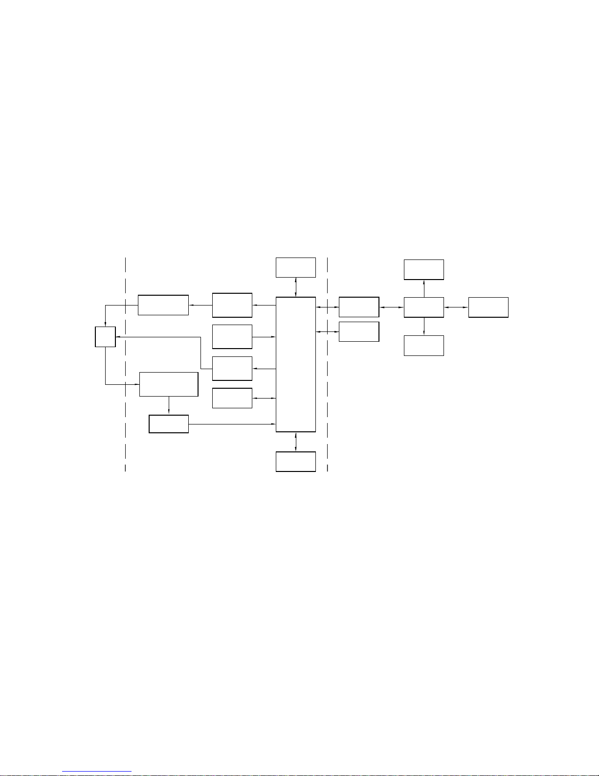These functions are shown in a block diagram in Figure 1-1.

REAL-TIME

CLOCK

CELL

EXTERNAL

POTENT IOSTAT

CURRENT AND

CHARGE TRANSDUCER

ANALOG FILTER

ADC

FUNCTION

GENERATOR

CONTROL

SOFTWARE

CELL AND

ELECTRODE

CONTROL

DATA

STORAGE

INTERNAL EXTERNAL

MICRO

PROCESSOR

VIDEO

CONTROL

RS-232

INTERFACE

I/O PORT

Figure 1-1. Block diagram of the BAS 100B/W Electrochemical Workstation.

LASER

PRINTER

PERSONAL

COMPUTER

DIGITAL

PLOTTER

DATA

STORAGE

1-1

Page 6

Sweep Techniques

Linear Sweep Voltammetry with linear and log output Cyclic Voltammetry

Step Techniques

Chronoamperometry Chronocoulometry

Pulse Techniques

Differential Pulse Voltammetry and Polarography Normal Pulse Voltammetry and Polarography Sampled Current Polarography

Square Wave Techniques

Barker Square Wave Voltammetry and Polarography Osteryoung Square Wave Voltammetry

A.C. Voltammetric Techniques

Sinusoidal A.C. Voltammetry and Polarography Phase-Selective Sinusoidal A.C. Voltammetry and Polarography Second-Harmonic Sinusoidal A.C. Voltammetry and Polarography Triangular Wave A.C. Voltammetry and Polarography Differential Triangular Wave A.C. Voltammetry and Polarography

Hydrodynamic Techniques

Rotating Disk Voltammetry Hydrodynamic Modulation

Stripping Techniques

Barker Square Wave Stripping Voltammetry Differential Pulse Stripping Voltammetry Linear Sweep Stripping Voltammetry Osteryoung Square Wave Stripping Voltammetry

Time Base

Amperometric Differential Pulse Triple Pulse

Miscellaneous

Bulk Electrolysis with Coulometry Electrocapillary Curve Impedance Programmable Potential Wave Form

Table 1-1. Electrochemical repertoire of the BAS 100B/W.

1-2

Page 7

Features

Thirty-eight techniques

•

PC control through Windows interface

•

Interaction with other Windows applications

•

Point & click user interaction

•

High resolution graphics

•

100 µV potentiostat resolution

•

True charge to voltage converter for chronocoulometry

•

Hardware interfaces with Voltammetric Cell Stand, Controlled Growth

•

Mercury Electrode, Low Current Module, Power Module, Rotating Disk Electrode and A.C. Impedance Module Control of stirring, inert gas purging and mercury drop knock & dispense

•

Multiple experimental runs and averaging

•

Automatic and manual peak finding routines

•

Anson, Cottrell and Tafel plots

•

Laser printer and digital plotter output

•

Multiple data set display and printing

•

Digital smoothing by Moving Average, Least Squares and Fourier Transform

•

Integration, differentiation, semi-integration and semi-differentiation

•

Background subtraction

•

Standard math operations

•

Data storage (binary and text formats)

•

Macro capability

•

Specifications

Firmware

Programmed ROM 192 KB RAM 116 KB Video RAM 6 KB

I/O

Cell stand port Custom port for control of BAS Cell Stands

and Controlled Growth Mercury Electrode

Accessories port Custom parallel port for control of BAS

Modules and other accessories

Data link port RS-232C serial port for communication

between 100B and remote PC Analog output Potential and current Analog input Potential

1-3

Page 8

Potentiostat

Output compliance voltage

12 volts minimum

Applied voltage range -3.276 volts to +3.276 volts Minimum potential step size 100 microvolts Absolute accuracy Reference input impedance >10

2.5 millivolts

ohms Maximum output current 190 milliamperes Risetime <2 microseconds Slew rate 10 Volts/microsecond minimum Stability 500 microvolts/day Effects of ±10% input

power line variation 100 microvolts maximum

Noise and ripple 100 microvolts RMS maximum

Current to Voltage Converter

Maximum current 190 milliamperes Ranges 100 milliamperes/volt

10 milliamperes/volt 1 milliamperes/volt 100 microamperes/volt 10 microamperes/volt 1 microampere/volt 100 nanoamperes/volt

Fullscale output

10 volts

Input voltage drift 500 microseconds/day maximum Input current drift 25 picoamperes/day maximum Conversion rate 20,000 conversions/sec or

50 microseconds/conversion Absolute accuracy 1% fullscale Resolution 0.05% fullscale

Charge to Voltage Converter

Maximum charge 3.2 millicoulombs Range 10 microcoulombs/volt (auto range)

General

Input voltage 110 volts, 120 volts, 220 volts, 240 volts Alternating Current 50 or 60 Hertz Input power 720 watts maximum 1 power outlet 120 volts Alternating Current @ 2A total.

1 microcoulombs/volt

100 nanocoulombs/volt

1-4

Page 9

Minimum Personal Computer Requirements

Processors 80386, 16 MHz

80387, 16 MHz Memory 2 MB RAM Hard drive 80 MB Floppy drives 1.2 MB 5.25”

1.44 MB 3.5”

Ports 2 serial

1 parallel Mouse PS/2 Monitor 14” color VGA

Unpacking and Inspection

Carefully unpack the BAS 100B/W from the shipping containers. Examine all packing materials before discarding it. Inspect all parts for obvious damage. Compare items received with the packing documents.

Damaged Shipments

If any damage has occurred whether obvious or concealed, all claims must be made to the carrier, usually within 15 days of your receiving the shipment; otherwise, the carrier may not honor the claim. Once the item has been assigned to a carrier for shipment, the carrier is responsible for its safe delivery. The following are some guidelines to follow when damage is discovered. You should contact the carrier directly for specific claim procedures.

United Parcel Service (UPS), Parcel Post, Air Parcel Post

1. Retain container, packing material, and broken item for inspection by the

carrier.

2. Write or phone BAS with our order number, the data received and a

description of the damage. BAS will do everything possible to expedite repair or replacement of the items damaged.

Air Freight, Express or Truck

1. Contact the local agent of the transportation company immediately and

request an inspection.

2. Retain the container, packing material and damaged goods until the

examining agent has made an inspection report.

In all of the above cases, do not return damaged goods to BAS without first contacting our customer service personnel for a Return Authorization Number

1-5

Page 10

(RA#). When a defective part is returned to BAS, the RA number immediately identifies you as the sender and describes the item being returned. To avoid confusion, BAS refuses all unauthorized return shipments.

Product Warranty

Bioanalytical Systems, Inc. (BAS) warrants equipment by the company to be free from defects in material and workmanship for a period of 1 year from the date of shipment, except as provided hereinafter. This assumes normal usage under commonly accepted operating parameters. BAS agrees to either repair or replace, at its sole option and free of part charges to the buyer, any parts of such instrumentation which, under proper and normal conditions of use, prove to be defective within 1 year from the date of shipment. Electrochemical cells and working electrodes are warranted for 60 days. This warranty and remedy are given expressly and in lieu of all other warranties, expressed or implied, of merchantibility or fitness for particular purpose and constitutes the only warranty made by BAS.

BAS neither assumes or authorizes any person to assume for it any other liability in connection with the sale, installation, service or use of its instrumentation. BAS shall have no liability whatsoever for special, consequential or punitive damages of any kind from any cause arising out of the sale, installation, service or use of its instrumentation.

All products manufactured by BAS are tested and inspected prior to shipment. Upon prompt notification by the Buyer, BAS will correct any defects in warranteed equipment of its manufacture either (by our option) by return of the item to our factory, or shipment of a repaired or replacement part. BAS will not be obliged, however, to replace or repair any piece of equipment that has been abused, improperly installed, altered, damaged or repaired by others. Defects in equipment do not include decomposition, wear or damage by chemical action or corrosion.

Limited obligations covered by this warranty include:

a. In the case of instruments not of BAS manufacture, the original

manufacturer’s warranty applies.

b. Shipping charges under warranty are covered only in one direction. The Buyer

is responsible for shipping charges to the factory, if return of the part is required.

c. Expendable items including (but not limited to) carbon paste, reference

electrodes, source lights, panel lights and fuses are excluded from this warranty.

1-6

Page 11

Warranty Card

Each BAS analyzer system is shipped with a warranty card which should be completed and returned by the end user. This card will enable us to identify and contact the individual responsible for the operation of the instrument. Please return the card as soon as possible so that we may inform you of product updates and other pertinent technical information.

Extended Warranty Agreement

BAS offers an extended warranty “Full Protection Service Agreement” to customers purchasing this system. Please contact you Sales Representative or the Service Department at BAS for further details.

Service Information

Bioanalytical Systems provides a skilled staff available to solve you technical and equipment-oriented problems. For service, call (765) 463-4527 during normal working hours (Eastern Standard Time the year round) and ask for Customer Service. The operator will route your problem to the correct individual. Following discussion of your specific difficulties, an appropriate course of action will be described and the problem will be resolved accordingly.

Do not return any products for service until a Return Authorization Number (RA#) has been obtained. The RA# identifies you as the sender and describes the problem you are having in full detail. All correspondence and shipments should be sent to:

Service Department Bioanalytical Systems, Inc. 2701 Kent Avenue West Lafayette, IN 47906 RA# ________________

1-7

Page 12

2. Installation

The installation of the BAS 100B/W Electrochemical Workstation can be divided into 2 parts: installation of the BAS 100B Electrochemical Analyzer and installation of the Personal Computer (PC). These will be considered in turn.

2.1 Installation of the BAS 100B Electrochemical Analyzer

Placement

As the Electrochemical Analyzer stands in a vertical position, it requires little bench space. However, adequate space should be left near the Analyzer for the PC and any other accessories (e.g., Cell Stands, Low Current Module, Rotating Disk Electrode). In addition, the area in front of the Analyzer should not be obstructed, as an airflow through the Analyzer is required for cooling.

Power Requirements

The Analyzer can be powered by any of the following A.C. voltages: 100V, 120V, 220V, 240V. The A.C. frequency may be either 50 or 60 Hz. The main power source in the location must be the same as the voltage selected in the power cord connector on the rear panel of the Analyzer (see Figure 2-1). For best results, an isolated power line is recommended.

All Analyzers are configured for the correct voltage and frequency for the "SHIPPED TO" destination. If the instrument is going to be operated at a voltage other than the standard voltage for the "SHIPPED TO" area, then a change must be made to the input power connector. The instructions for changing the voltage requirements are discussed below.

All the peripheral devices requiring power (e.g., plotter, printer, C2 Cell Stand) can be powered by 110/120V and 50/60 Hz by plugging then into the power outlet on the rear panel of the instrument.

110/120 Volts and 60 Hz Operation

110/120V and 60 Hz are the standard power requirements for the Analyzer and its peripheral devices. All of these can be plugged into the usual mounted, main power outlets.

2-1

Page 13

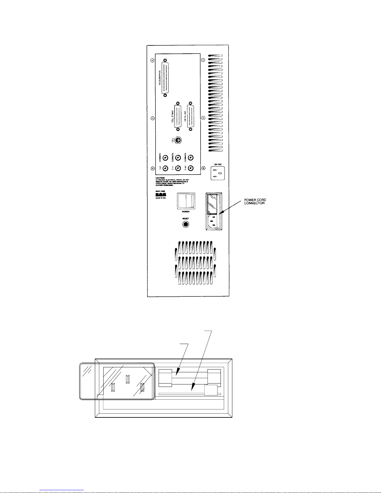
Figure 2-1.

omitted).

Rear panel of BAS 100B (the ports that are not required for the BAS 100B/W are

VOLTAGE SELECT PCB

FUSE

FUSE PULL

Figure 2-2.

Power connector and voltage select.

2-2

Page 14

Before plugging the Analyzer power cord into a power socket, confirm that the correct voltage has been selected in the power cord connector. This is done as follows:

a. Remove the power cord from the power cord connector (the location of this

connector is shown in Figure 2-1).

b. Slide the plastic window to the left to expose the voltage select printed circuit

card (this card is shown in Figure 2-2). The orientation of this card in the connector determines the voltage option.

c. If the number printed on the outer edge of the board does not correspond to

the available voltage, pull out the card (the fuse must be removed first), and turn it (either by rotation or inversion) such that the desired voltage is exposed on the outside edge of the top board. Reinsert the board and replace the fuse.

If the Analyzer is operated from a power outlet without a safety ground connection, an appropriate adapter must be used. The ground connection of this adapter must be securely fastened to an external earth ground for safety and proper operation. A proper ground connection cannot be overemphasized.

The power cord is shipped as a separate item and must be plugged into the connector on the rear panel (Figure 2-1). To insert the power cord into the power socket, push up the plastic window and plug in the female end of the power cord. The plug type on the male end of the power cord may vary depending on the country of destination.

The A.C. frequency is checked for 50 or 60 Hz operation during the Self-Test sequence of the Analyzer that occurs on power up (see Section 5.12 for more details on this Self-Test).

220/240V and 50 Hz Operation

220/240V and 50 Hz are the standard power conditions available in many countries. The Analyzer can operate using such power sources and some of the peripheral devices and accessories can accommodate this power. Check each peripheral device for it's power requirements. A device requiring 110V can be ruined when plugged into a 220V power source.

To check or change the power requirements of the Analyzer:

a. Remove the power cord from the power cord connector (the location of this

connector is shown in Figure 2-1).

2-3

Page 15

b. Slide the plastic window to the left to expose the voltage select printed circuit

card (this card is shown in Figure 2-2). The orientation of this card in the connector determines the voltage option.

c. If the number printed on the outer edge of the board does not correspond to

The A.C. frequency is checked for 50 or 60 Hz operation during the Self-Test sequence of the Analyzer that occurs on power up (see Section 5.12 for more details on this Self-Test).

Cell Connection

The cell lead cable is the group of wires that connects the Analyzer electronics to the electrodes of the electrochemical cell. One end of this cable plugs into CELL on the rear panel of the Analyzer (Figure 2-1) and the other end is attached to the electrodes. This may be a direct connection using the general purpose cable sent with the Analyzer or one for attachment to a cell stand such as the BAS C3 Cell Stand.

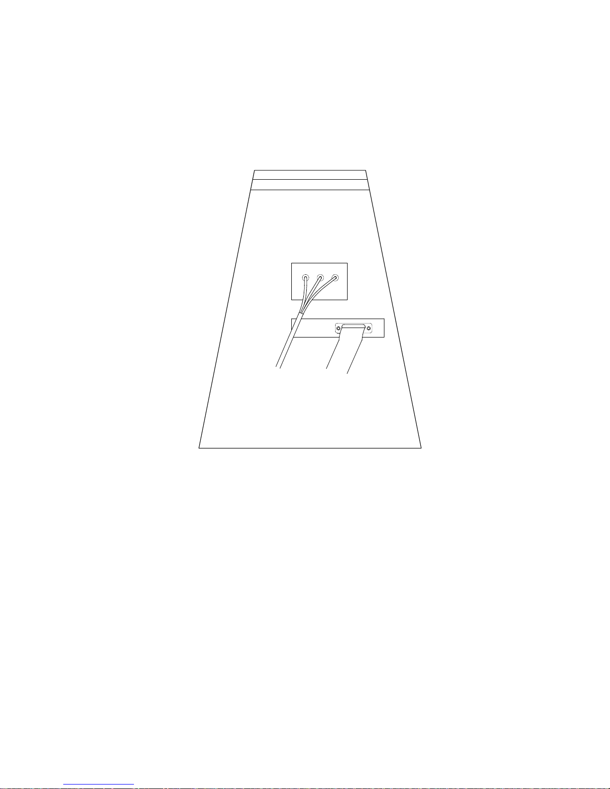
The general purpose cell cable terminates with alligator clips that attach directly to the cell electrodes (Figure 2-3). There are 3 electrode leads and 1 grounded (shielding) lead.

The color code is:

Black covered wire: Working Electrode lead Red covered wire: Auxiliary Electrode lead White covered wire: Reference Electrode lead Bare or Black wire w/lug Earth ground connector

2-4

Page 16

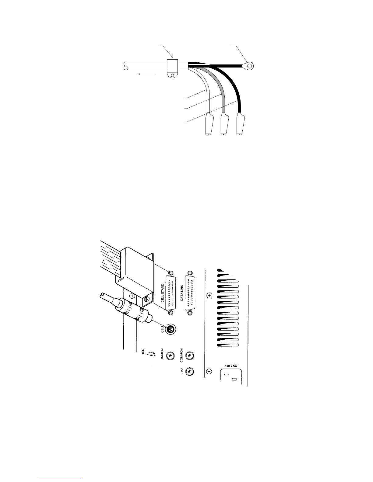
STRAIN RELIEF GROUND (BLACK)

TO CELL CONNECTOR

ON BAS 100A

REFERENCE (WHITE)

AUXILIARY (RED)

WORKING (BLACK)

Figure 2-3.

Cell (electrode) end of cell cable.

A plastic mounting lug near the end of the cell cable provides strain relief by preventing movement of the line or cell.

Cell Stand Connector

This connector is used to control cell stand functions (i.e., stirring, gas purging and drop knocking), and is plugged into the CELL STAND port on the rear panel of the Analyzer (Figure 2-4).

Figure 2-4.

Attaching cell lead to BAS 100B.

There are 3 cell stand configurations available for the BAS 100B/W Workstation (through

Setup

in the

File

menu). One configuration (C2) is for the BAS C2 Cell

2-5

Page 17

Stands, and the other two are for the BAS Controlled Growth Mercury Electrode (CGME) - one for the SMDE mode (

CGME

(

). The

SMDE

configuration can also be used with the PARC 303A

SMDE

) and one for the CGME mode

SMDE.

BAS C2/C3 Cell Stand

The purging and stirring functions on the BAS C3 Cell Stand can be controlled manually or through the BAS 100B/W. The REMOTE port on the rear of the Cell Stand is connected via a 25 pin ribbon cable to the CELL STAND port on the rear panel of the Analyzer.

CGME

The purge and stir functions on the BAS Controlled Growth Mercury Electrode (CGME) can be controlled manually or through the BAS 100B/W. In addition, the knock and dispense routines required for the SMDE and CGME modes are controlled by the BAS 100B/W, and the

Cell Stand

option in the

Setup

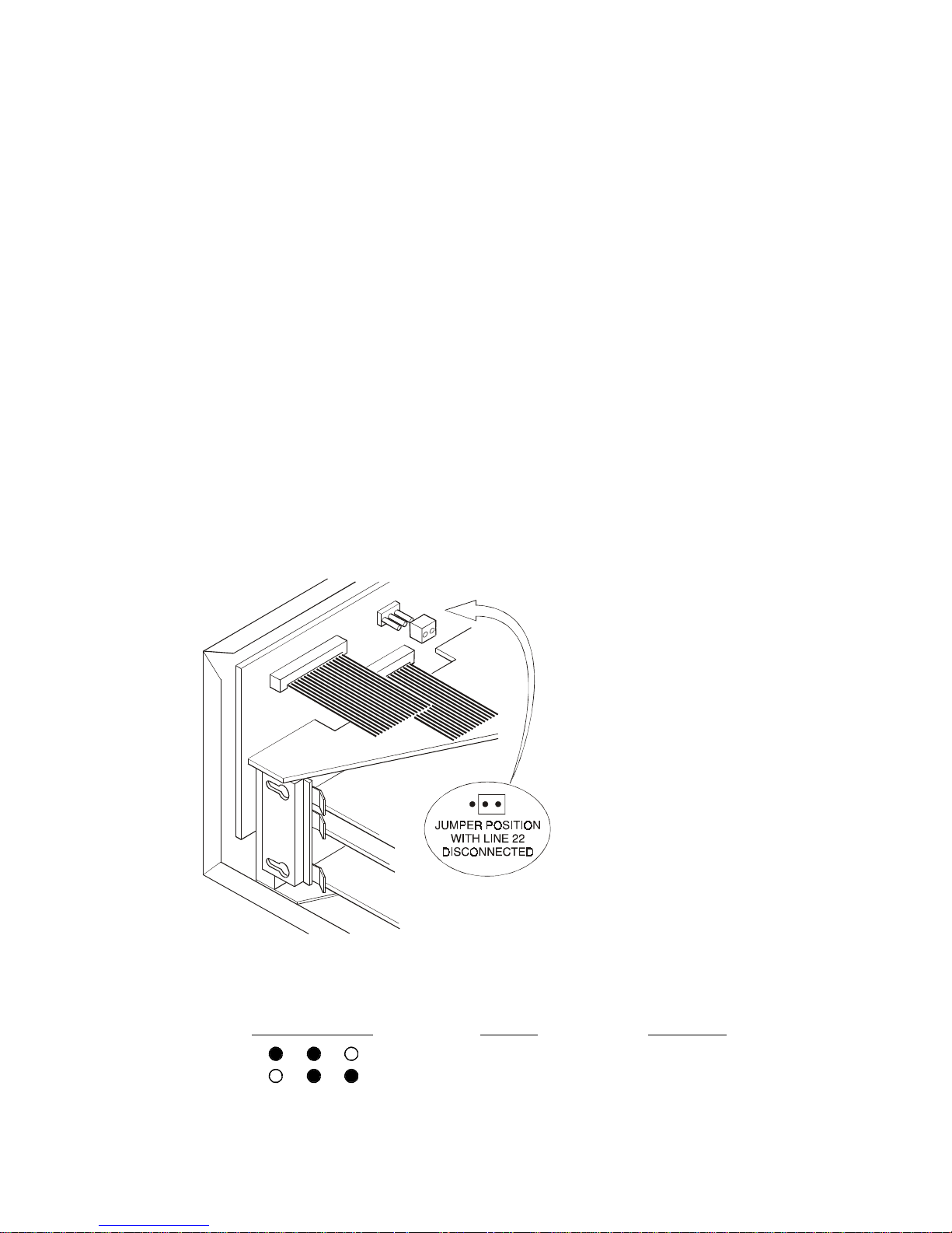
dialog box must be set appropriately. The jumper on the back panel board for Line 22 of the control cable must be in the connected position (Figure 2-5).

Figure 2-5.

panel board of the BASI100B.

Line 22 of the Cell Stand control cable must be disconnected via a jumper on the back

Jumper Position Line 22 Cell Stand

Connected CGME Disconnected PAR 303A

2-6

Page 18

PARC Model 303A SMDE

The jumper on the back panel board (Figure 2-6) must be in the disconnected position for the PARC 303A. The BAS 100B/W can be used to control the stirring, purging, knock and dispense of the PARC 303A SMDE. Two connections are required (Figure 2-6):

Figure 2-6.

Connector on 100B

PARC cell connections.

To CELL

To CELL STAND

Connector on 100B

1. Connect the CELL STAND port on the rear panel of the Electrochemical

Analyzer to the INPUT port on the rear panel of the 303A via a 25 pin ribbon cable (P/N EF-1600). Line 22 of this cable must be disconnected for proper operation of the 303A. Early versions of the BAS 100A require line 22 to be cut. Later versions of the BAS100A and BAS 100B have a jumper on the back panel board to disconnect line 22. However, line 22 is connected on the BAS 100B/W, so the position of the jumper must be switched in order for the knock function of the 303A to operate,

2. Use the Analog Signal Cable (P/N EW-8096) to connect CELL on the rear

panel of the Electrochemical Analyzer to the ELECTRODE TEST POINTS on the rear of the 303A. The pins on the end of the cable are inserted into the mounted sockets. The color code is:

Black pin into the WORK Electrode Socket Red pin into the CNTR Electrode Socket

2-7

Page 19

White pin into the REF Electrode Socket

Electrocapillary measurements can be done using the 303A, but only with manual control; that is, toggle the drop function switch to the DME position just before the start of the experiment and toggle to either SMDE or HMDE when the scan is complete.

Accessories

This port allows the BAS 100B/W to sense and control the accessories and special function modules available to the BAS 100B/W. The accessories that use this custom port are the Low-Current Module, the Power Module/Potentiostat, the Rotating Disk Electrode and the AC Impedance Module. More details are included in each of the accessories operations manual.

Plotter/Printer Connection

These ports are now obsolete as plotting and printing is controlled by the Windows software. Plotters and printers should therefore be connected to the PC.

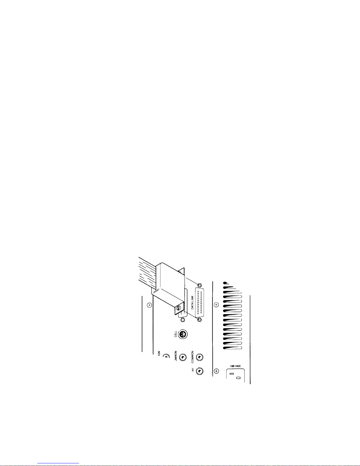
Data Link

This port is used to communicate with the external PC via the cable and one of the serial communication ports (COM ports) on the PC via a standard RS-232C cable. This connection is shown in Figure 2-7.

Figure 2-7.

Attaching remote control (DATA LINK) cable to rear panel connnector.

2-8

Page 20

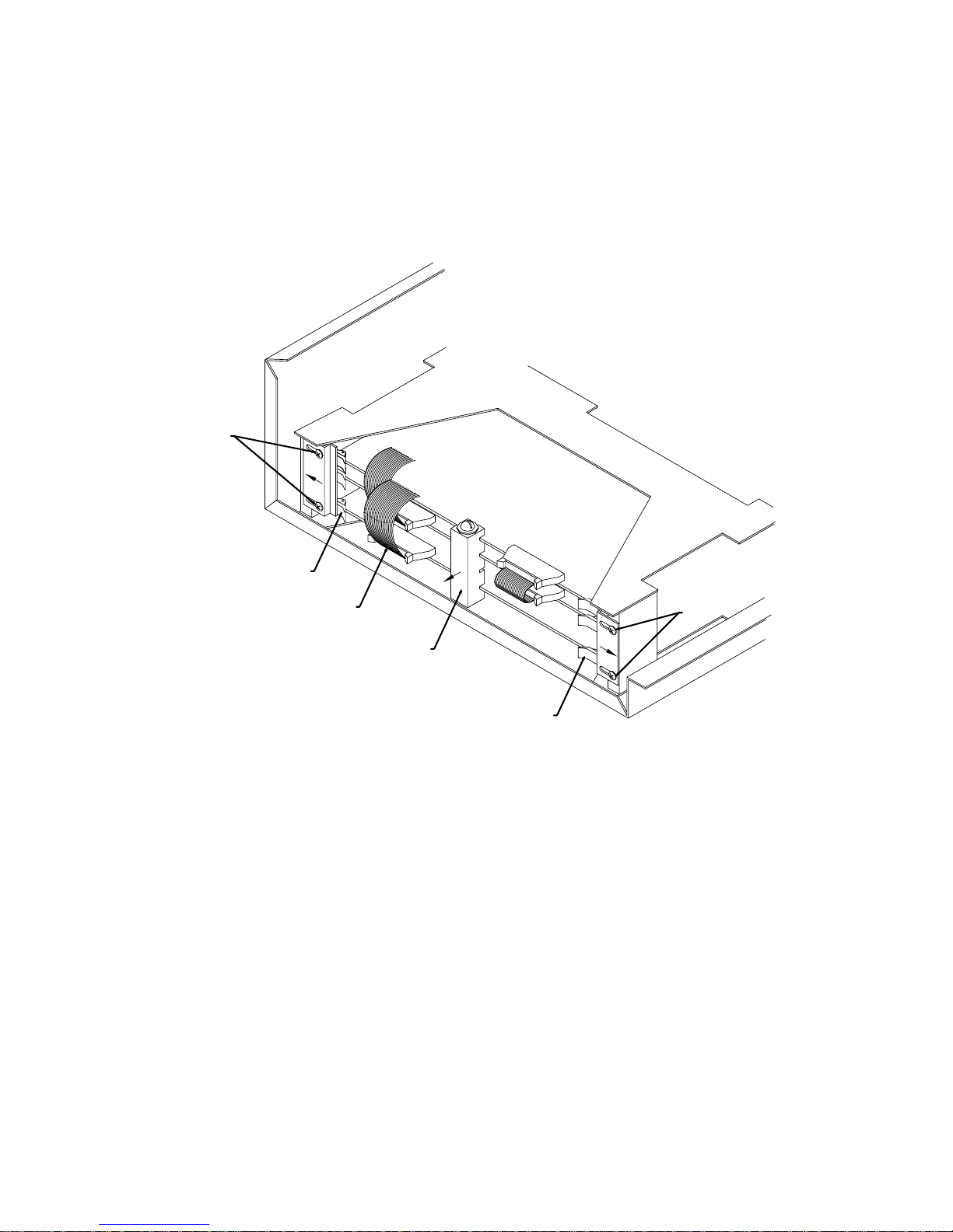
2.2 Installation of CPU Board for BAS 100B/W Upgrade

PC BOARDS A. Analog Board B. I/O Board C. CPU Board

a) Remove white plastic board support (item 1). NOTE: early BAS 100A models

do not have the board support.

b) Loosen four designated screws (Item 2) on card rack and slide card retainer

plates outward.

c) Remove necessary ribbon cables (Item 3) by pressing ejectors outward from

connectors and remove.

d) Remove the old CPU board (bottom board) by pressing ejectors (Item 4)

outward and pulling boards straight out. NOTE: Many of the large scale integrated circuits are static sensitive. DO NOT place on plastic (e.g., bubble pack), carpeting or other surface which may have static build-up.

e) To reinstall the new CPU board, reverse the above procedure.

2-9

Page 21

2.3 Installation of Replacement ROMs in the BAS 100B/W

a) Remove the CPU as described in section 2.2

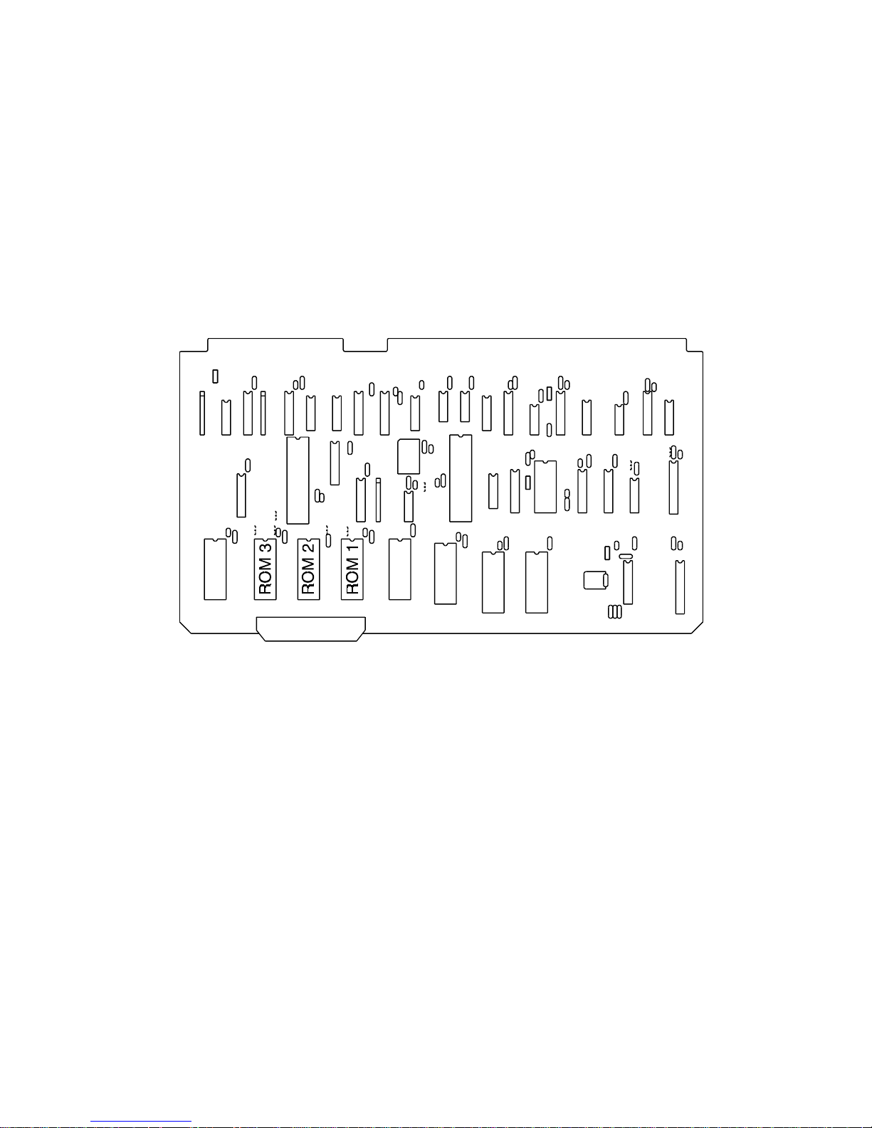
b) Lay CPU board (Figure 2-8) on a flat surface. Components of the CPU board

are sensitive to static. Do not lay the board on carpeting, plastic (e.g., bubble wrap), or other surfaces that build up static charge.

Figure 2-8. CPU Board

c) Carefully pry ROM 1 out of its socket - be careful not to bend the legs of the

chips.

d) Properly align new ROM1 on the socket and press in. It is imperative that the

chip oriented as shown in Figure 2-8 (notched end away from the board edge with the ribbon cable connector). Be careful not to bend the legs and ensure that all the legs are inserted into the socket.

e) Replace ROMs 2 and 3 in the same way, and reinstall board.

2-10

Page 22

2.4 Personal Computer (PC) Installation

Machine Requirements

The BAS Windows software was written for use on BAS PCs. Other IBM compatible PCs may be able to run this software, but there are no guarantees.

The MINIMUM requirements for the BAS Windows software are:

a) 80386 processor running at 16 MHz, together with a math co-processor.

b) Hard disk drive.

c) MS-DOS version 5.0 or greater.

d) MS-Windows 3.1 or greater.

e) VGA monitor.

f) 2 serial interface connectors (one for communication with the Electrochemical

Analyzer and one for plotting using a serial port plotter)

g) 1 parallel interface connector for a parallel port printer (e.g., laser printer).

h) PS/2 mouse (do NOT use a serial mouse).

PC Connections

The important connections are:

a) VGA video display connector.

b) Keyboard connector

c) PS/2 mouse connector

d) Power cable connectors for the system unit and the monitor. The female ends

the two power cables should be connected to these. The male end of the monitor power cable should be plugged into the power socket on the rear of the system unit. The male end of the system unit power cable should be connected to a grounded power strip or outlet. It is VERY important to check that the correct voltage has been chosen using the line voltage connector (110/220 V). It is also advisable to install a line noise/surge protector between the power source and the PC.

2-11

Page 23

e) Serial interface connectors (COM1 and COM2). These can be used for any

serial RS232C device; for the BAS 100B/W, they are used for communication with the Electrochemical Analyzer and for plotting. COM1 is connected with the DATA LINK port on the rear panel of the Analyzer, and COM2 is connected with the chosen plotter.

f) Parallel interface connector. There is one parallel interface connector (LPT1),

which is used to connect a parallel printer via a parallel printer cable.

Setting up the BAS PC is described in more detail in the enclosed User's Guide.

Once the above connections have been made, the system unit and monitor can be powered up.

Software

All BAS PCs are shipped with MS-DOS, MS-Windows and BAS 100W Windows software already loaded on the hard disk drive, which is labeled as the C: drive. If a non-BAS PC is being used, the BAS 100W Windows software is loaded according to the following instructions (which assume that MS-DOS and MS-Windows have already been loaded).

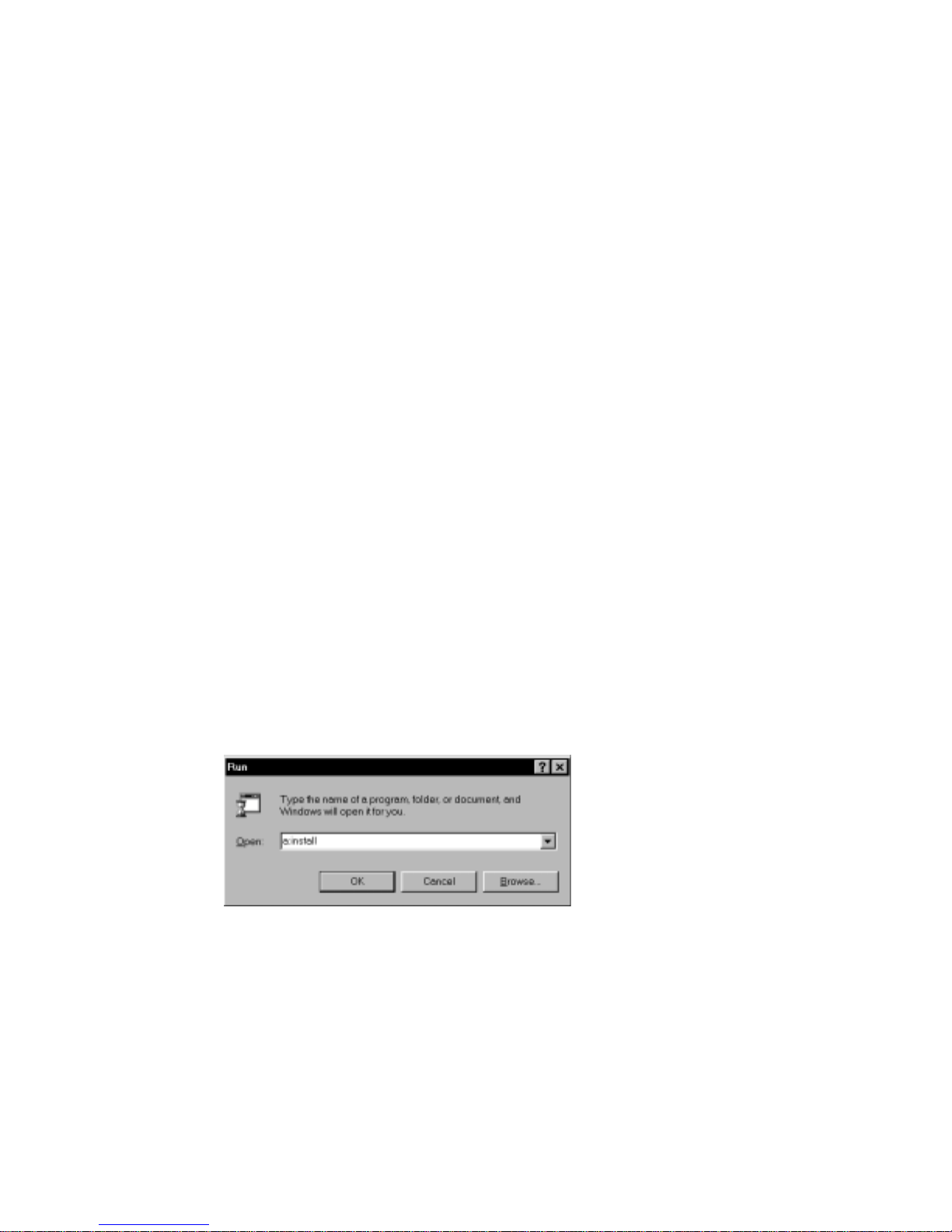
1. Enter by Windows by typing win at the DOS prompt.

2. Insert the BAS 100W software disk into the appropriate floppy disk drive.

3. Select

b:install

Figure 2-9. Run dialog box.

4. The

Run

) in the

Install

from the

dialog box will appear (Figure 2-10). Unless specified otherwise,

File

menu in the

Command Line

Program Manager

, enter

(Figure 2-9), then click OK.

a:install

the BAS 100W software will be installed in the \BAS100W directory created by the installation routine. The BAS 100W icon will be installed in the BAS Programs group. Click

Install BAS100W

to start the installation.

(or

2-12

Page 24

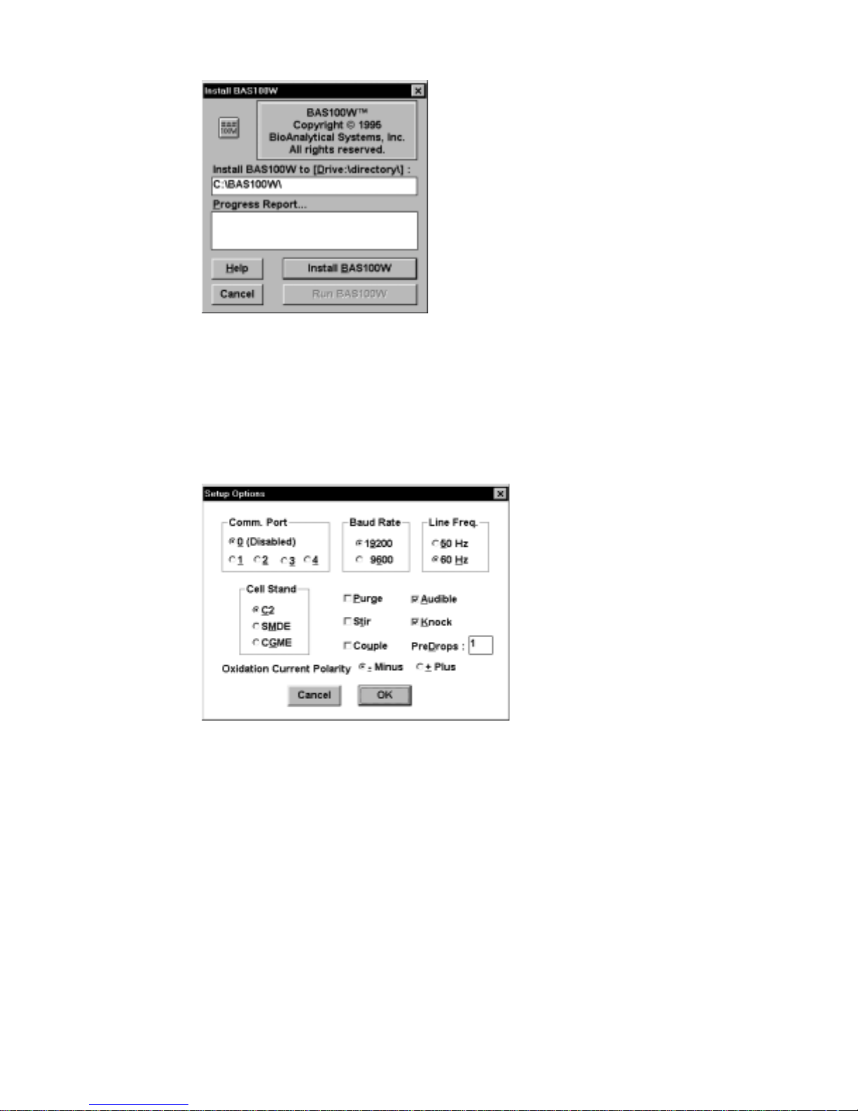
Figure 2-10. Install dialog box.

5. The BAS 100W software is opened by double-clicking the BAS 100W icon.

Before any operation, it is advisable to check that the communication parameters are correct. These are contained in the

Setup

dialog box in the

File

menu (Figure 2-11).

Figure 2-11. Setup

Setup

The

communications options are as follows:

Com Port

Baud Rate

Line Freq.

dialog box.

This specifies which PC communications port is connected to the BAS 100B. A value of 0 disables the communication.

This specifies the rate at which information is transferred between the PC and the BAS 100B. This specifies the line frequency of the local A.C. voltage. The selected frequency determines the default

Sample Width

2-13

for pulse experiments.

Page 25

Cell Stand

The BAS 100B/W can control the purging and stirring for BAS Cell Stands and the BAS Controlled Growth Mercury Electrode (CGME). The knock/dispense routines for the

CGME

modes of the Mercury Electrode are also controlled by the BAS 100B/W, so the option must be set accordingly (the

SMDE

Cell Stand

SMDE

option

and

can also be used for the PAR 303A SMDE).

The other parameters in the

Setup

dialog box are discussed in Section 3 (see page

3-4).

Once the

Setup

communication parameters have been checked, the

Electrochemical Analyzer can be powered up. The system is now ready for use.

Printer/Plotter Configuration

Although a printer/plotter can be selected using the

Options dialog box (see Section 9.2), the appropriate driver must first be installed. The drivers for older models of printers/plotters are contained on the Windows 3.x disks, and are installed using the Printer dialog box in the Control Panel. However, the drivers for more recent models have to be provided by the printer manufacturer, and require a different method of installation; however, explicit instructions are typically provided with the printer, so installation should cause no problems.

2-14

Page 26

3. File Menu

3.1 File Dialog Box

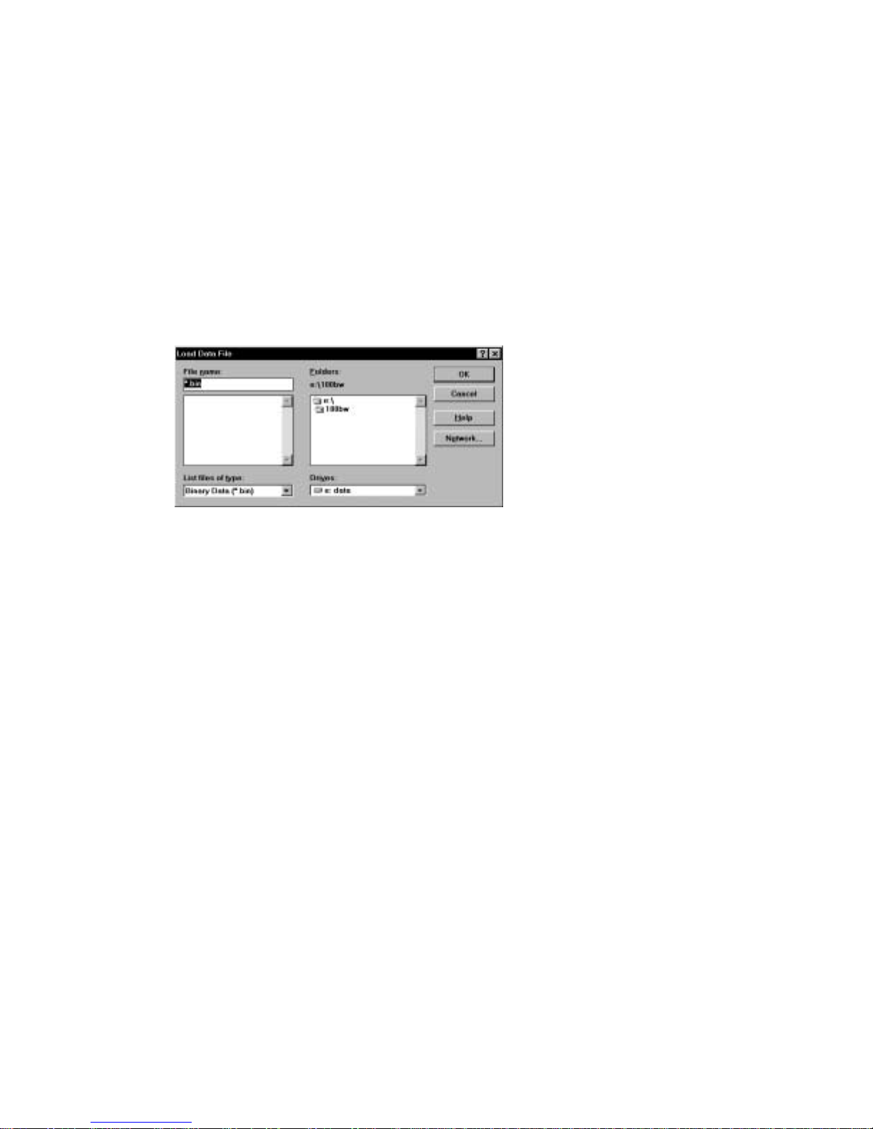
The BAS 100W software uses standard Windows file dialog boxes for transfer of data files between disk drives and the main memory and for other file manipulation.

Load Data File

The

dialog box is shown in Figure 3-1.

Figure 3-1. File

File Name

File List box

List Files of Type

dialog box.

This field is used to specify the name of the file, which can be either typed or selected from the Once the file name is shown in the field, click activate the selected operation.

This list box lists all files of the type specified in the

Files of Type Directories List

file name or click on the file name and then click

To select two or more data files (for commands that accept multiple files), drag the mouse over the desired files names or hold down the last files in the group. If the files are separated, hold down

<Ctrl>

the the same directory.

BAS 100W recognizes its own files by using specific extensions, such as .BIN, .TXT or .MOD. If only one extension type is permitted, then that type of file is selected automatically. When more than one type of file is allowed, the program initially selects the previous choice, but allows selection of the alternate file types.

field from the sub-directory selected in the

field. To select a file, double-click on the

<Shift>

key while selecting. Multiple files must be in

key as you select the first and

File List box

[OK]

below.

List

3-1

Page 27

Directories List

The current pathname is shown above this list box, and is updated when a different disk drive or directory is selected. The path is changed by selecting one of the directories shown in this list and then clicking [OK] or pressing

Enter

< directory). Files in the selected directory (which is now the default directory) will then be listed in the

> (alternatively, you can double-click on the desired

Files List

Drive Select

This drop-down list box show the current disk drive. To select a different drive, click on the [ and select the desired drive.

Down-Arrow

3.2 Load Data

Load Data

The in either binary (.BIN) or text (.TXT, .CRL, .SPC and .TAB) format. .TXT files from earlier BAS File Service programs can also be loaded.

command reloads a data file previously saved by the 100W software,

3.3 List Data

List Data

The of the data without having to save the data as a text file. During listing, you can press

Enter

Pause

[

> to Pause the listing or press <

] or [

command lists the data currently in main memory. This allows review

Esc

> to Cancel further lines or click on

Cancel

] in the BAS100W Listing box.

3.4 Save Data

] box

Data can be saved in the BAS100W's compact binary (.BIN) format or in the text (.TXT, .CRL, .SPC and .TAB) format, which can be read by other programs.

3.5 List Text File

List Text File

The (.TXT, .CRL, .SPC and .TAB) format. Any text file having the .TXT, .CRL, .SPC and .TAB extension can be listed. During listing, you can press < listing or press < BAS100W Listing box.

command is used to list data files previously saved in the text

Esc

> to Cancel further lines or click on [

3-2

Pause

Enter

> to Pause the

Cancel

] or [

] in the

Page 28

3.6 Convert Files

Convert Files

.CRL, .SPC and .TAB) formats. Up to 100 files can be selected. After the file(s) have been selected, the program prompts you to confirm the number of files. The text format is determined by the

As the converted files are listed on the screen, you can press < listing or press < BAS100W Listing box.

Note

: Files cannot be connected from one text format to another text format.

is used to convert data files between the binary (.BIN) and text (.TXT,

Text Data Format

Esc

> to Cancel further lines or click on [

dialog box (3.10).

Pause

Enter

> to Pause the

Cancel

] or [

3.7 Delete Files

Delete Files

selected, the program prompts you to confirm the number of files.

As the deleted files are listed on the screen, you can press < listing or press < BAS100W Listing box.

can delete up to 100 files of any type. After the file(s) have been

Enter

> to Pause the

Esc

> to Cancel further lines or click on [

Pause

] or [

Cancel

] in the

3.8 Rename Files

Rename Files

The changed. After the file(s) have been selected, the program prompts you to enter the new file name.

command allows the names of up to 100 files of any type to be

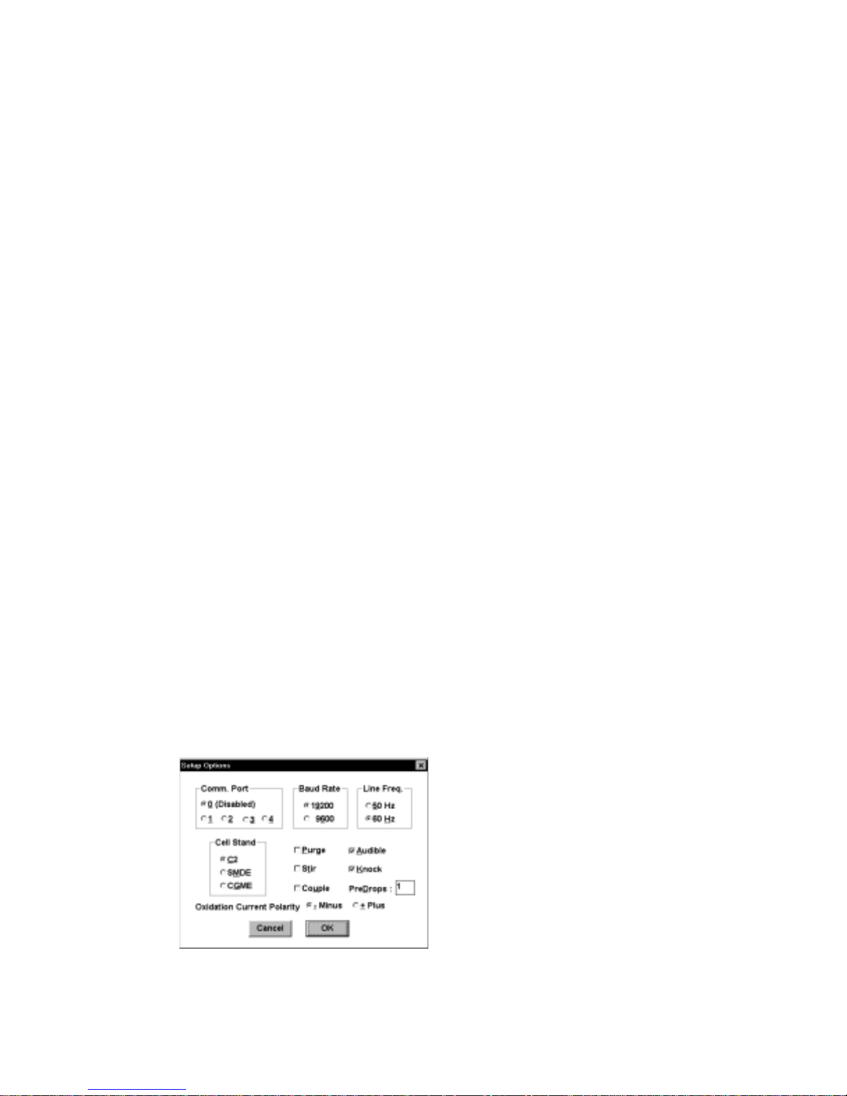
3.9 Setup

Figure 3-2. Setup

dialog box.

3-3

Page 29

Com Port

This specifies which PC communications port is connected to the BAS 100B. A value of 0 disables the communication.

Baud Rate

Line Freq.

Cell Stand

Purge/Stir Couple

This specifies the rate at which information is transferred between the PC and the BAS 100B.

This specifies the line frequency of the local A.C. voltage. The selected frequency determines the default

Width

for pulse experiments - 17 ms for 60 Hz and 20 ms

Sample

for 50 Hz (1 line cycle is selected in order to minimize line frequency interference).

The BAS 100B/W can control the purging and stirring for the BAS Cell Stands and the BAS Controlled Growth Mercury Electrode (CGME). The knock/dispense routines for the

SMDE

are also controlled by the BAS 100B/W, so the option must be set accordingly (the

and

CGME

modes of the Mercury electrode

Cell Stand

SMDE

option can also

be used for the PAR 303A SMDE).

This activates purging/stirring between experiments.

This couples purging and stirring during the deposition step of stripping experiments.

Audible Knock

PreDrops

This activates a beep before and after each run

This synchronizes the drop knock/dispense of a mercury electrode with the end of the potential pulse. If

Knock

is not checked, then no knock or dispense will occur before or during the experiment when using the modes (however, if

Growth

dialog box is checked, then the valve is held open,

Controlled DME

SMDE

in the

CGME

Controlled

but no knock occurs). This is the number of mercury drops dispensed from a

mercury electrode before the start of an experiment (provided the

Knock

option is checked). For

experiments using the BAS CGME, the number of

Drops

number entered. For

Pre Drops

depends on the selected drop size as well as the

CGME

experiments, the number of

delivered will match the number entered,

SMDE

Pre

regardless of the drop size, and entering 0 will allow the same drop to be used for multiple experiments (except in polarography experiments).

3-4

Page 30

Oxidation Current Polarity

This specifies the sign of an oxidation current - positive (IUPAC convention) or negative (classical convention).

3.10 Text Data Format

When data are listed on the screen, or saved in a text format, each data point includes an X value (typically potential or time), and one or more Y values (typically current or charge). The delimiters.

Text Data Format

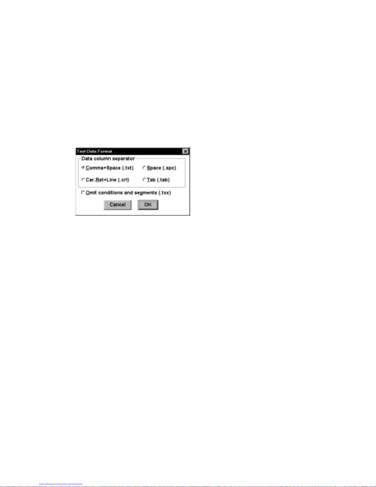
dialog box provides a selection of data column

Figure 3-3. Text Data Format

The file extension for each format option is indicated in parentheses. The default delimiter is

segments

separators between segments. These files cannot be loaded back into the 100W program.

Comma + Space

will allow conversions of

dialog box.

, and the default extension is

.bin

to a text format without the header and the

.txt

Omit conditions and

3.11 Exit

Upon exiting the software, the method parameters for the last experiment are saved in a TEMP.MOD file, and the sizes and positions are saved in a 100W.INI file.

Setup

options,

Graph Options

and

Colors

, window

3-5

Page 31

4. Method Menu

4.1 Load/Save Method

This allows an experimental contain the parameters entered in for the

Results Options

boxes.

. These operations are performed using standard Windows file dialog

Method

(.MOD) to be

4.2 Select Mode

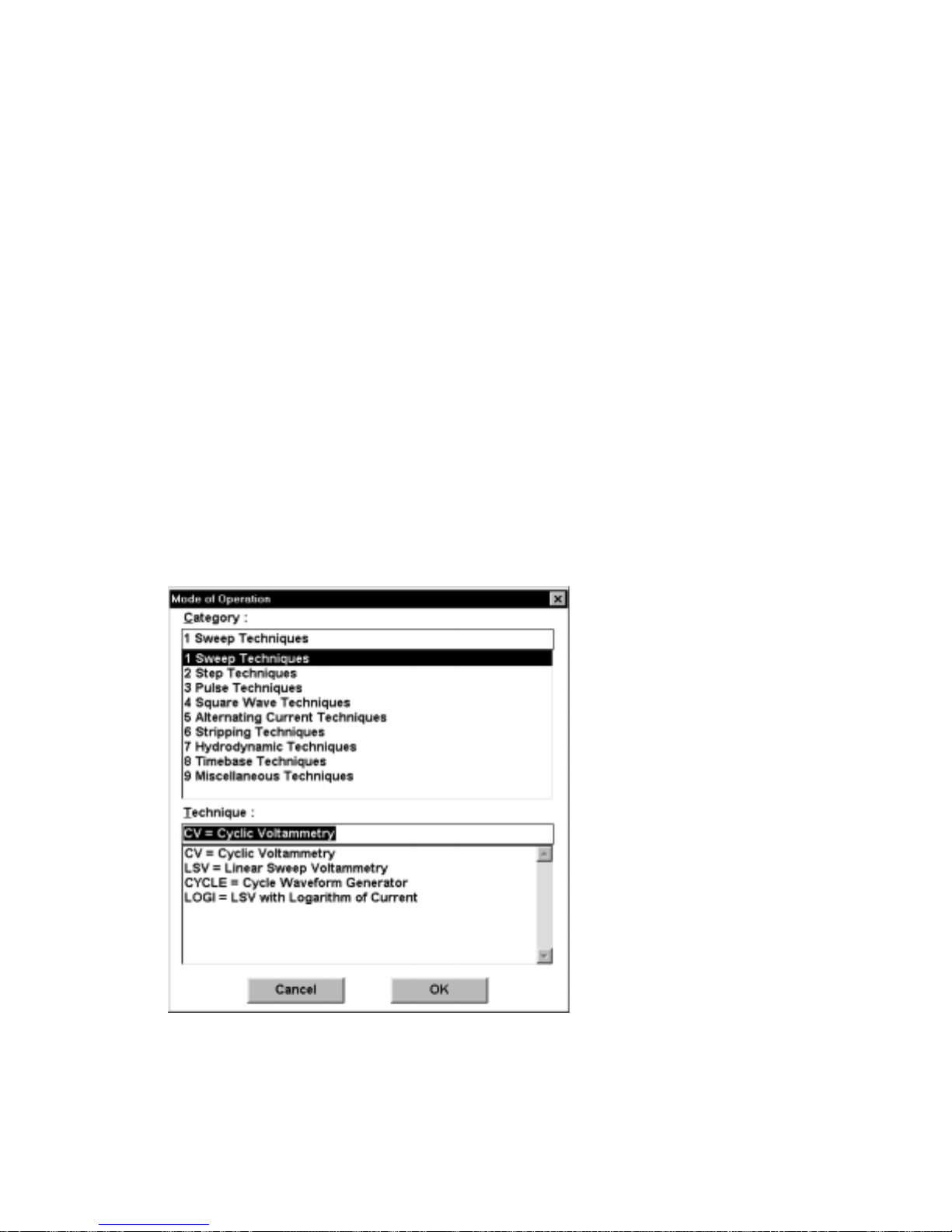
There are 38

Category

Technique

is highlighted, the modes associated with that

Load

Method

list box (Figure 4-1). The required

and

General Parameters

ed or

Control

Save

d. Method files

menus, and the

dialog box

Figure 4-1. Select Mode

dialog box.

4-1

Page 32

4.3 General/Specific Parameters

Some electrochemical techniques require many different parameters, and this can cause confusion. For ease of operation, the parameters are divided into two categories,

General

and

Specific

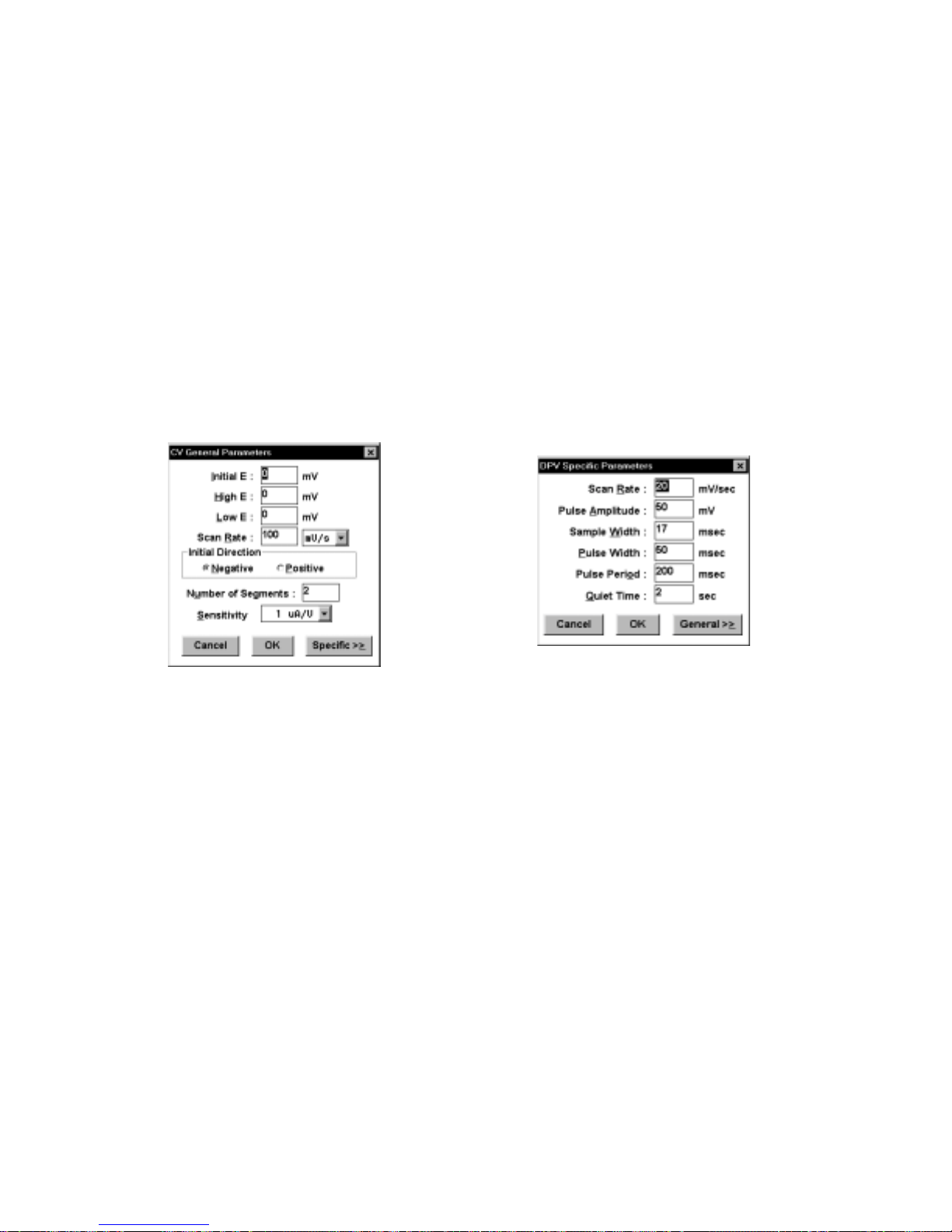
General Parameters

standard values for these parameters. potential range ( of the current-to-voltage converter) (Figure 4-2). Other

Scan Rate

the hydrodynamic and stripping experiments.

Figure 4-2. General Parameters

dialog box for

must be set by the user for each experiment, as there are no

General parameters

Initial E, Final E, High E

(for linear sweep experiments) and the

Low E

and

Figure 4-3. Specific Parameters

dialog box for

always include the

) and the

General Parameters

Sensitivity

Rotation Rate

DPV.

(the gain

include

(for

Specific Parameters

for most conditions. They do not have to be set by the user for each experiment, although values other than the default values can be entered. typically include the parameters that define the potential wave form (for techniques other than linear sweep, potential step and time based); for example, the

Frequency

and

Pulse Width

and

have default values, which have been chosen to be reasonable

Specific Parameters

of square wave and sinusoidal potentials and the

Pulse Period/Drop Time

for pulse experiments (Figure 4-3).

Sample Width

Amplitude

4.4 List Parameters

List Parameter

The

Parameters

command lists the present values of the

4-2

General

and

Specific

Page 33

4.5 Filter

Analog filtering is used during data acquisition to lower the output noise. The analog filtering in the BAS 100B/W is a two stage network (Figure 4-4). The first stage is an RC filter, which is followed by a Bessel filter. The filtering characteristics of each stage can be varied, and are related to the time scale of the technique being used. The capacitor in the RC filter should be chosed to give a time constant (RC) that is at least 10 times smaller than the time scale of the experiment. Similarly, the cut-off frequency for the Bessel filter must be at least 10 times larger than the frequency of the electrochemical technique being used. If too much filtering is used, then significant distortion of the experimental data can occur.

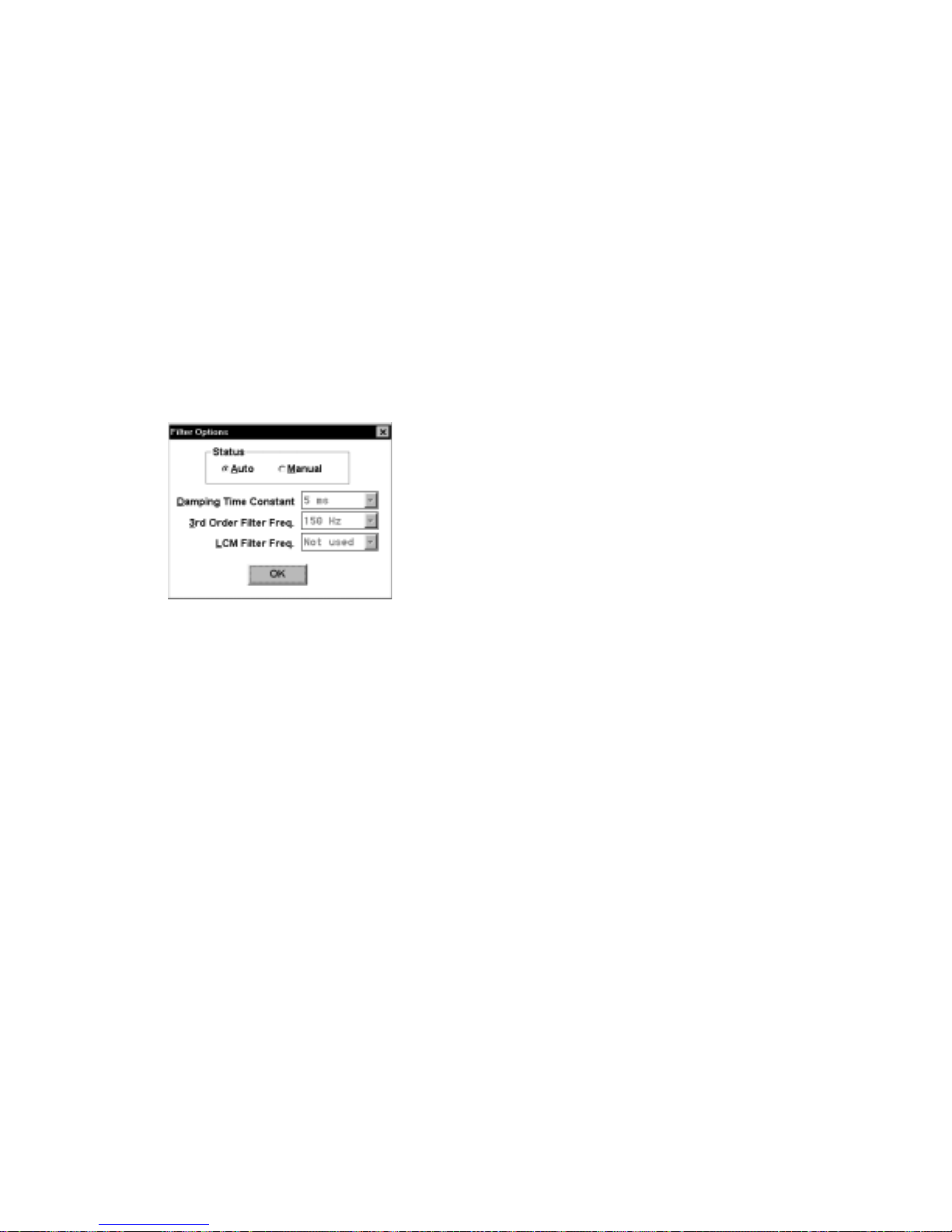
Figure 4-4. Filter

The amount of filtering used can be determined automatically using the (this is the default option). It is generally advisable to use this option. However, the filters can be changed by the user through the selected fromdrop-down list boxes).

When the Low Current Module (LCM) is being used, the BAS 100B/W filters are disabled by the filters can be re-enabled using the

dialog box.

Auto

option, and the only the

Manual

LCM Filter

option.

Auto

option

option (the desired filter is

is used. The BAS 100B/W

4-3

Page 34

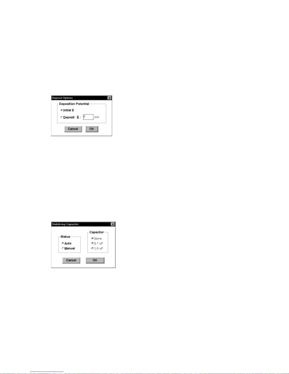
4.6 Deposit Options

Deposit Options

The default for this parameter is the initial potential for the potential scan ( If some other potential is required, then the the required potential should be entered in the

Figure 4-5. Deposit Options

is used to define the deposition potential for stripping experiments.

Initial E

Deposit E

dialog box.

option should be selected, and

field (Figure 4-5).

4.7 Stabilizing Capacitor

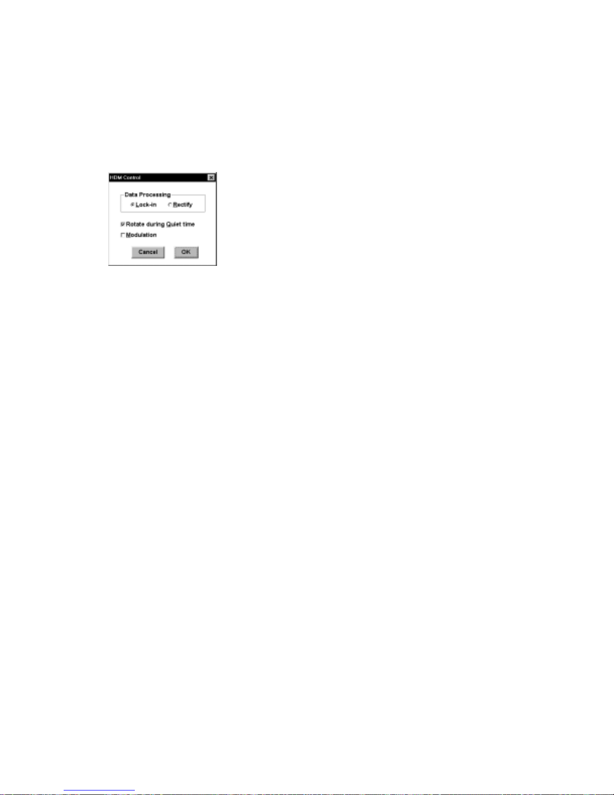
A stabilizing capacitor is only required when using iR compensation, or for Bulk Electrolysis (BE) experiments. In both these cases, the or 1 µF capacitor into the circuit. The when using the with caution, since the addition of capacitors can affect the frequency response of the system.

Manual iR

option (Figure 4-6). The

Manual

option generally only needs to be used

Auto

Manual

option switches a 0.1 µF

option should be used

Figure 4-6. Stabilizing Capacitor

dialog box.

4-4

Page 35

4.8 Hydrodynamic Modulation

This specifies additional parameters for the Hydrodynamic Modulation ( technique (Figure 4-7).

Figure 4-7. Hydrodynamic Modulation

Data Processing

Rotate during Quiet Time

dialog box.

This specifies the method for handling the A.C. current output (

A finite length of time is required for the Rotating Disk Electrode to reach the selected rotation rate. Therefore, rotation is started during the Quiet time to ensure that the desired rotation rate has been attained when the potential scan is started.

Lock-in

Rectify

HDM

)

Modulation

This option switches on the modulation of the rotation rate.

4.9 Controlled Growth

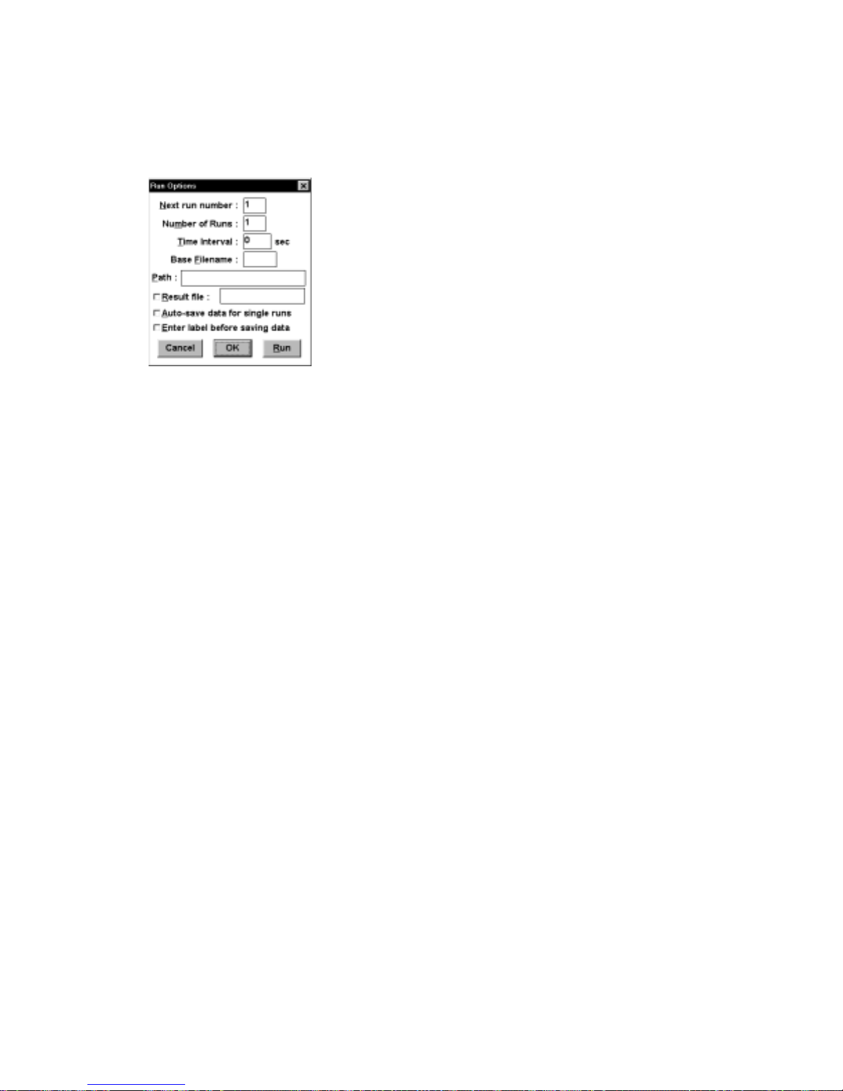
This specifies drop growth parameters for the CGME mode of the BAS Controlled Growth Mercury Electrode for both pulse and stripping experiments (Figure 4-8).

CGME

The box for this item to be activated.

CGME

In the (pulses). There are three parameters that defined this series: duration of each pulse), pulses). These parameters are entered under

mode must be selected for the

mode, the mercury drop is grown using a series of valve openings

Number of Pulses

Cell Stand

Delay Time

and

Knock and Dispense Control

options in the

(the time between the

Setup

Pulse Width

dialog

(the

4-5

Page 36

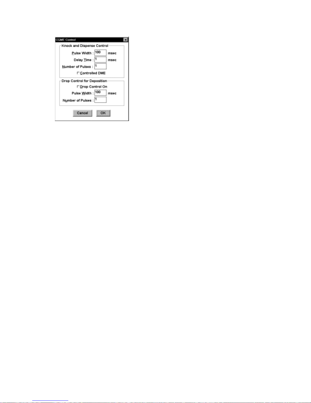
Figure 4-8. Controlled Growth

dialog box.

The CGME can also be used as a DME when in the

Controlled DME

check box. This will open the valve at the start of the experiment

CGME

mode by activating the

and close it at the end of the experiment. The mercury will flow freely during the course of the experiment and the of the drop knocker) is selected using

Dropping Time

Specific Parameters

(i.e., the time between activations

(the natural drop time at low potentials in aqueous solution for the standard 150 µm capillary is typically slightly less than 1 s).

CGME

The

mode can also be used for anodic stripping voltammetry (Z. Kowalski and J. Migdalski, Electroanalysis 4 (1992) 915). The mercury drop is grown incrementally during the deposition step using a series of pulses. The drop size is again determined by the under the

Deposit Time

Drop Control for Deposition

and the

Number of Pulses

45 s of the

Deposit Time

Pulse Width

Number of Pulses

is 4, then the pulses will occur at the beginning and at 15, 30 and

and the

. The incremental growth in activated by clicking

check box. The Delay Time is determined by the

Number of Pulses

: if the

Deposit Time

, which are entered

is 60 s and the

4-6

Page 37

5. Control Menu

5.1 Start Run

This command (or F2) initiates the experiment. During runs, all menus are disabled except the Control commands: Start Run, Hold/Continue Run, Reverse Scan and Stop Run. After completion of the run, the menus are re-enabled according to the present mode and data set.

After a single run, the graph is replotted according to the present Graph Options if data are available (the Step and Cycle modes never produce data). The Filename label that appears above the graph is cleared to indicate that the data are not yet saved. For single runs, the data are not saved automatically; the Save Data command in the File menu must be used.

5.2 Hold/Continue

Clicking this option (or F3) holds the experiment at a given potential. The experiment can be restarted by clicking the option again.

5.3 Reverse Scan

The command (or F4) reverses the direction of the potential scan for CV experiments. The data for experiments in which this function has been used should be saved as text files (binary files will not save the revised potential values correctly).

5.4 Stop Run

This command (or F5) stops the experiment.

5-1

Page 38

5.5 Run Options

Figure 5-1. Run Options dialog box.

This command allows some automation when running experiments.

a) It Runs and the Time Interval between the runs must be specified by the user

(Note: the Time Interval is in addition to the time required to transfer the data to disk). The data files are stored automatically after the run in the binary (.BIN) format (the Base Filename and the Path (drive and directory) must be specified by the user). The first run starts immediately after [OK] is selected, unless a warning is given that existing files will be overwritten by this operation. During each run, the title of the graph shows the filename of that run. Between runs, a small dialog box shows the filenames of the previous and next runs, and the time remaining before the next run. The filenames of the completed runs are listed in the Main window.

If the Find peaks after run box is checked (Results Options in the Analysis menu), a Results Graph and Results List is produced after each run, rather than a Single Graph. Note that is may require additional time to calculate the results: therefore, if the Time Interval between runs is critical, this option should be unchecked.

Pressing <Esc> at any time during a series of Multiple Runs will abort the present run and any further runs.

The number of the first run can be specified using Next Run Number. This allows a previous set of multiple runs to be continued.

b) If a Result file name is entered, the program creates a file containing one result

line for each run, nicely formatted according to the Data Column Separator option selected in the Text Data Format dialog box. Both multiple and single runs append lines to the result file if it is enabled. Comma+Space format (.CSV extension) and Tab format files are very easy to import into Excel. For convenience of importing, all text labels are extracted from the Result file,

5-2

Page 39

leaving just the data values. Note: Car. Ret + Linefeed format works differently than the other formats--it saves an exact copy of all lines listed on the screen during each run.

c) The data from single experimental runs can be save automatically by clicking

Auto-save data for single runs. The Path and Base Filename must be specified.

d) Clicking Enter label before saving data allows the user to specify a label for the

data file of the experiment just run (a dialog box is displayed after each run). This can be used for both single and multiple runs. However, for multiple runs, the time available for entering the label is limited by the Time Interval. If it is less than 10 seconds, this option is not available. For longer Time Intervals, once the time has expired, the data are saved with whatever label has been entered, and the next run is then started. After a label has been entered, and [OK] has been clicked, the standard timer dialog box appears to count down any excess time that remains.

5.6 List Run Data

When this command is checked in the menu, the experimental data are listed on the screen during runs if the data rate is slow enough (as determined by the software) to allow time for listing.

5.7 iR Compensation

In any potentiostatic experiment, it is assumed that the potential drop across the interfacial region at the working electrode is the same as the potential applied between the reference and working electrode. However, this is not true, since there is some iR drop between these two electrodes due to solution resistance. This resistance can be lowered by addition of supporting electrolyte, and in many cases does not need to be considered. However, there are instances where it is detrimental to the experiment; in these cases, it can be compensated for electronically. On the BAS 100B/W, this is achieved by the iR Compensation command.

There are two stages to Auto iR Compensation on the BAS 100B/W (P. He and L.R. Faulkner, Anal. Chem. 58 (1986) 523):

a) measurement of the uncompensated resistance b) compensation and circuit stability testing

5-3

Page 40

Measurement of Uncompensated Resistance

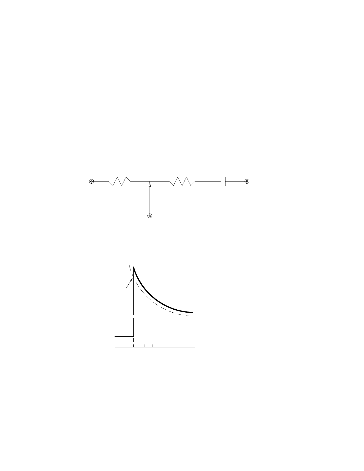
In this measurement, the electrochemical cell is considered to be electronically equivalent to an RC circuit; that is, the uncompensated resistance (R

with the double-layer capacitance (C

) (Figure 5-2). Since a Faradaic impedance

is not considered as part of this model, the test potential (Test E) must be at a value at which no Faradaic process occurs. A 50 mV potential step (∆E) is applied around this potential (i.e., Test E-25 mV to Test E+25 mV), and the current is sampled at 54 µs and 72 µs after the step is applied. The current decays exponentially, and the initial current (I

zero time (Figure 5-3). Since ∆E = I

) is calculated by extrapolating back to

oRu

measurement. To reduce any error, this measurement is performed 256 times, and the results averaged.

) is in series

, Ru can be calculated from this

Figure 5-2.

RC circuit used for calculation of the solution resistance.

-t/R C

i e

u dl

Figure 5-3.

Exponential decay of current response.

0 54 72

t/µs

5-4

Page 41

Ru/Ω

50.3 38 29 -42

100.4 94 92 -8.4 150 146 145 -3.3 200 198 198 -1.0 250 250 249 -0.4 300 302 301 +0.3 347 350 349 +0.6 401 406 404 +0.7 452 360 449 -0.7

Table 5-1. Measured resistance and time constant via exponential extrapolation (P. He and L.R. Faulkner, Anal. Chem. 58 (1986) 523).

measured RC

time constant/µs

measured Ru/Ω

error of R

measurement/ %

Table 5-1 shows the results of resistance measurements for various dummy cells using exponential extrapolation. There is very good agreement when the time constant is greater than 200 µ the time constant is below 100

s; however, the error in the extrapolation is large if

s, since the current has decayed significantly by

the time the response is sampled. Therefore, the Auto iR Compensation may not work when the uncompensated resistance is low, and/or the time constant is small.

Compensation and Circuit Stability Testing

Compensation is achieved by positive feedback into the potentiostat. However, problems due to circuit instability can arise, even when the degree of compensation is significantly less than 100%. Therefore, the positive feedback is applied in increments of the calculated uncompensated resistance: 5% increments up to 80%, 2% increments from 80% to 90%, and 1% increments thereafter. The stability of the circuit is tested after each increment. The degree of compensation is defined by the user (default = 100%).

In the stability test, a 50 mV potential step around Test E is again applied, and the current data are collected at a rate of 20000 points/sec for 50 ms. A baseline is measured by collecting data shortly before the potential step is applied, and these baseline values are subtracted from the potential step data to yield net current values.

As the percent compensation increases, the current response at first exhibits a "ringing effect" following exponential decay (Figure 5-4) which would eventually go into oscillation. The degree of pre-oscillation ringing can quantitated by a term defined as Overshoot, which the ratio of a minimum (net negative) current value (I

) to a maximum current value (I

min

Overshoot = (I

min/Imax

) x 100. The maximum allowable Overshoot value is

) expressed as a percentage: that is,

max

defined by the user (Default = 10%). If the measured Overshoot value is less than the maximum allowable value, then compensation is continued. If it is greater, and the desired level of compensation has not yet been achieved, a capacitor is

5-5

Page 42

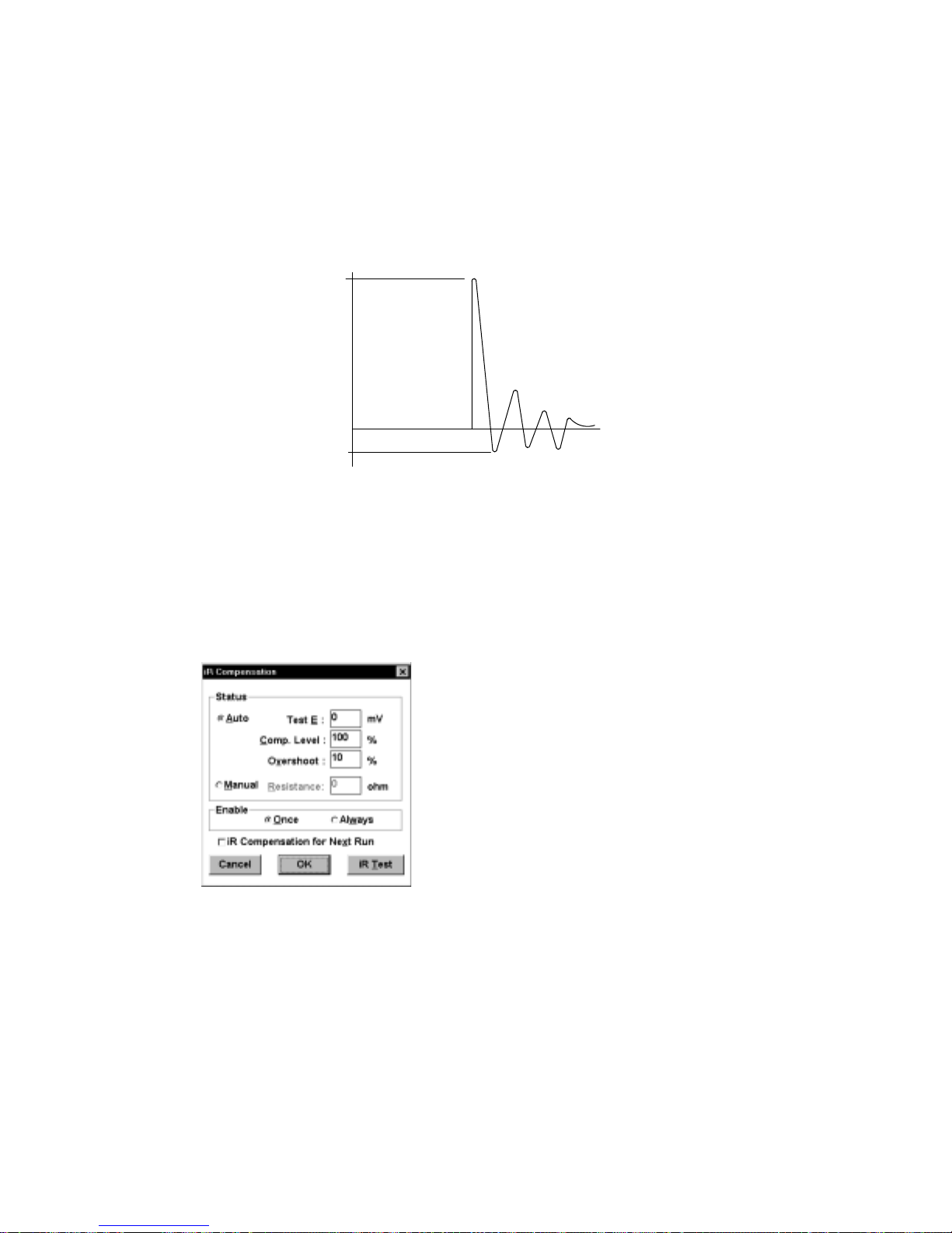
inserted between the reference and auxiliary electrodes to stabilize the circuit, and the testing is continued until the desired level of compensation is achieved or the Overshoot value is exceeded (if this occurs, the amount of compensation to be used in the experiment is slightly decreased from this value). One way to increase the level of compensation is to increase the Overshoot percentage. It is usually safe to go up to 40%.

max

min

Figure 5-4. "Ringing" of the current response.

If the desired compensation cannot be obtained using Auto iR Compensation, then a user-specified compensation resistance can be applied using the Manual option. If this option is used, then a stabilizing capacitor may also need to be selected manually (see Stabilizing Capacitor in the Method menu)

Figure 5-5. iR Compensation

1) Using Auto iR Compensation:

a) Select the Auto option from Status.

b) Select the appropriate option from Enable. If Once is chosen, then only

the next experiment performed will be iR compensated. If Always is selected, then the amount of compensation determined by the iR Test will

dialog box.

5-6

Page 43

be used for every subsequent run (Note: if Always is chosen, the instrument does not redo the iR Test before every run).

c) Before Auto iR Compensation can be used the iR Test must first be run.

This test requires three parameters values to be specified by the user:

Test E (this must be a potential at which no Faradaic process occurs) Comp. Level (the degree of compensation: default = 100%) Overshoot (the extent of instability allowed in the circuit: default = 10%)

d) Click iR Test . As the test is running, the following results are displayed

in the Main window:

Uncompensated resistance (R Cell RC constant (the product of R

)

and Cdl) (these are the results of the

resistance measurements)

R to be compensated (percentage of R

used in positive feedback)

Uncompensated R (uncompensated R remaining after compensation)

(these are the results of the stability testing)

e) Ensure that the iR Comp for Next Run check box is activated.

f) Click OK to exit.

2) Using Manual iR Compensation

a) Select the Manual option from Status.

b) Select the appropriate option from Enable.

c) Enter the desired Resistance.

d) Ensure that the iR Comp for Next Run check box is activated.

e) Click OK to exit.

5.8 Measure Rest Potential

This command measures the open circuit potential. This potential is particularly important in studies on corrosion (corrosion potential) and batteries (open circuit potential), and it can be used as the initial potential in voltammetry experiments.

5-7

Page 44

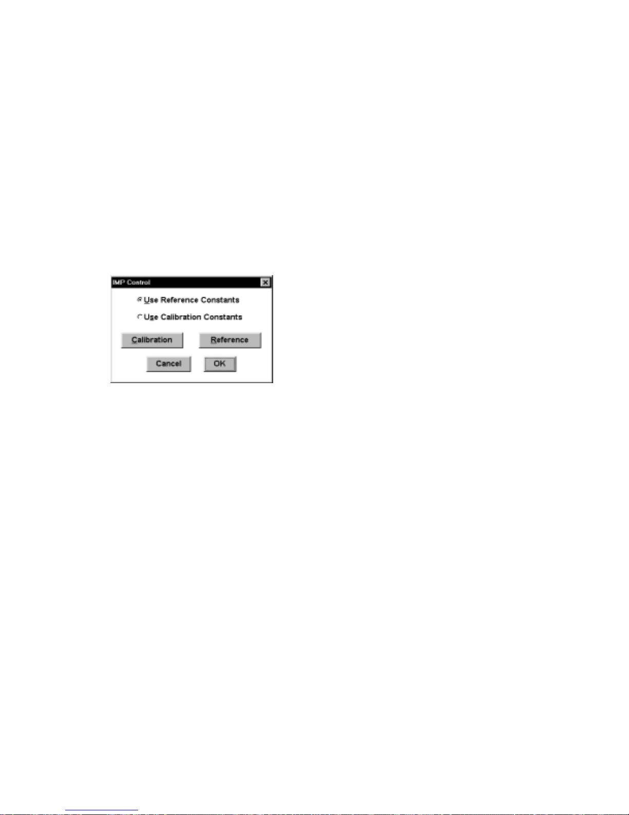
5.9 Measure Impedance

This command is used to calibrate the BAS 100B/W for impedance experiments (BAS Impedance Module required). This calibration requires a 1000 ohm resistor, which is connected to the working electrode on one side and the reference and auxiliary electrodes on the other. The Initial E (in the General Parameters) must be set to zero. The Reference command button calibrates the entire frequency range, using the default parameters. The results are stored in a calibration table in batterybacked RAM, so the Reference procedure does not have to be repeated for the lifetime of the battery. This calibration requires many hours, so is best done overnight. If the Impedance Module was purchased with the BAS 100B/W, this operation was done in the factory before shipping. If not, it must be done by the user.

Figure 5-6. Impedance Control dialog box.

The Calibration command button generates a special calibration table to be used under a given set of user-defined conditions (e.g., frequency range, amplitude). However, this calibration table is not stored in battery-backed RAM, and is lost when the main power is switched off. Once the calibration tables have been set up, either may be used (select the Use Reference/Calibration Constants).

During calibration, numerical values are displayed in the Run window. These values are meaningless, and should be ignored. Once the calibration has been completed, close the Run window and click OK.

5.10 Immediate Purge/Stir

The Immediate Purge/Stir command allows stirring and/or purging for a set length of time. Purging and stirring can be coupled by checking both boxes in the dialog box.

5-8

Page 45

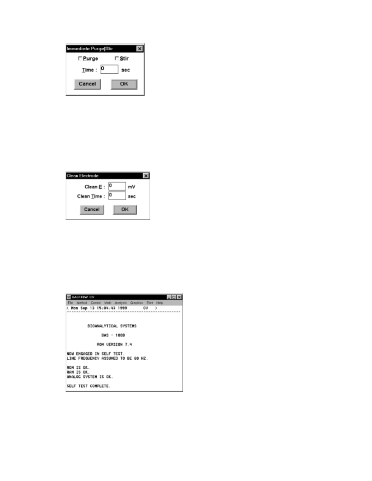
gure 5-7. Immediate Purge/Stir dialog box.

5.11 Clean Electrode

The Clean command is used to hold the electrode at a fixed potential for a set length of time without accumulating any data. This can be useful for generating clean, reproducible working electrode surfaces.

Figure 5-8. Clean Electrode dialog box.

5.12 Self-Test Hardware

This command initiates the potentiostat electronic self-test. The results of the test are displayed in the Main window (Figure 5-9).

Figure 5-9.

Self-Test Hardware

result.

5-9

Page 46

5.13 Cell On/Off

When Cell On is selected, the working electrode is connected at all times. When Cell Off is selected, the working electrode is only connected during experimental runs.

For most experiments, the cell should be off between runs, since there is more chance of damaging the instrument (and of personal injury when using the PWR-3) if the cell leads are connected/disconnected when the cell is on.

5-10

Page 47

6. Math Menu

6.1 Operators

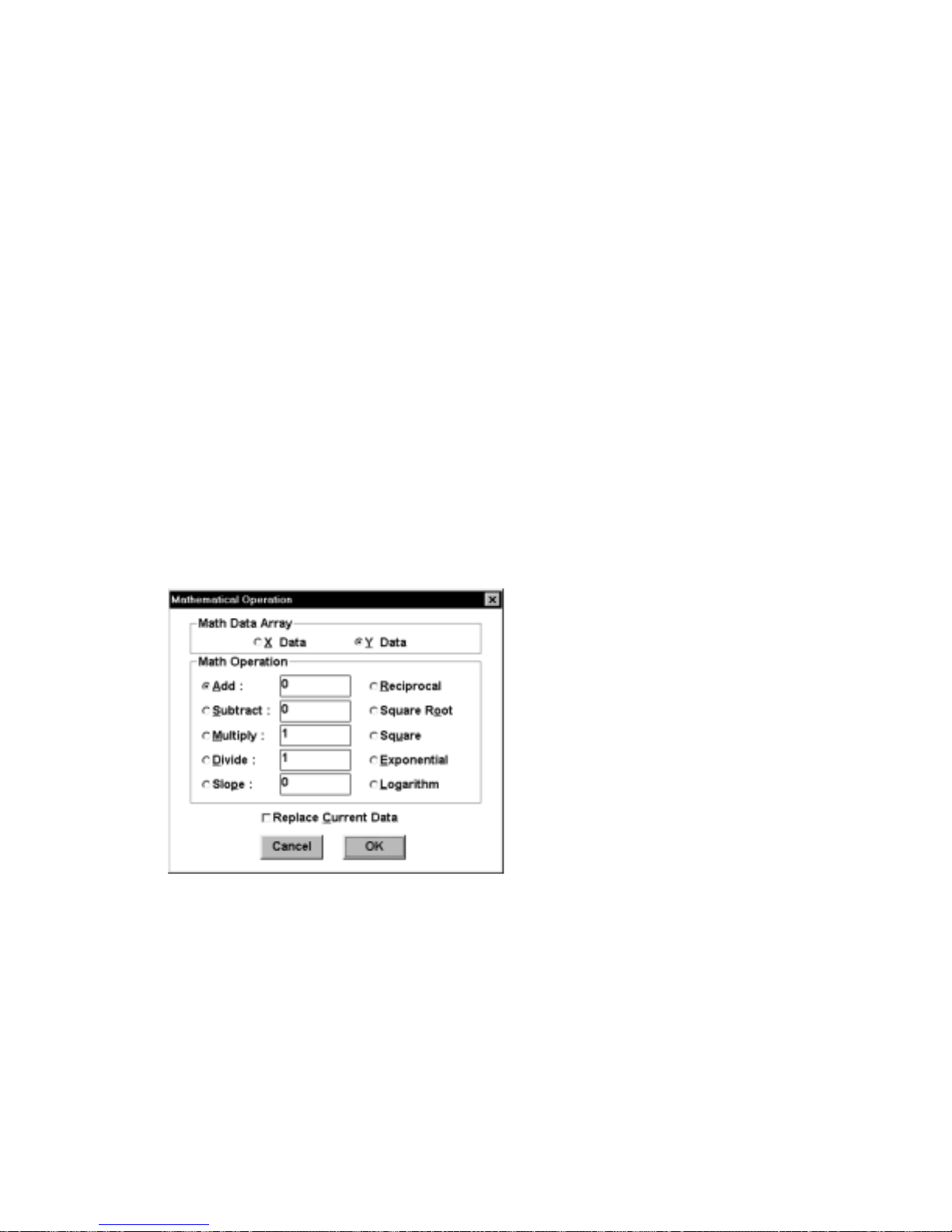
A variety of mathematical operations can be performed on either the X or Y data. These are addition, subtraction, multiplication, division, reciprocal, square, square root, exponent and logarithm (Figure 6-1). In addition, the slope of the baseline can be adjusted. Activating main memory. If this is not activated, the processed data can be displayed only once (after the math operation has been completed).

It should be noted that there is a difference in the way the X data is saved for binary and text files. In binary files, only the initial and final X points and the X sample interval are saved, and the remaining X data points are generated when the file is loaded. However, in text files, all the X data are saved. Therefore, processed X data can only be saved in the text format.

Replace Current Data

will transfer the processed data to

Figure 6-1. Operators

6.2 Smooth

The digital smoothing routines are used to remove unwanted noise from the electrochemical signal thereby improving the signal-to-noise ratio and giving more reliable information. In all data manipulation programs, attempts are made not to bias the signal. The major effect of the programs in the BAS 100W is the elimination of the higher frequency components of the signal, typically 10's of Hz and greater (the

dialog box.

6-1

Page 48

exact cutoff frequency depends on both the electrochemical and smoothing techniques). There are 3 methods for digital smoothing. These are:

a) a modified variable point linear smoothing routine ( b) a variable point least squares smoothing routine ( c) a Fourier Convolution smoothing routine (

Fourier Transform

Moving Average

Least Square

)

Moving Average

In the modified 5-point linear smooth, data is examined in 5 point blocks. Within each block, the first, second, fourth and fifth points are summed and divided by 4. This number (an averaged current value) replaces the third point in the block. The averaging routine moves up 1 point, and repeats the averaging sequence. This routine is repeated for all points.

The first 2 points of the data set are set equal to point 3 and the last 2 points of the data set are set equal to the third from last point. At times, this appears as spurious data points at the ends of the plot. This is unavoidable and is normal.

The only requirement for the number of points is a block is that this number is odd. Any odd number between 5 and 25 can be chosen on the BAS 100W - the larger the number of points, the greater the smoothing.

Least Squares

This digital smoothing function is based on the work of Savitzky and Golay: A. Savitzky and M. J. E. Golay, Anal. Chem. 36 (1964) 1627 - 1639. The smoothing is a quadratic least squares operation working on data blocks of n points (where n is any odd number between 5 and 25).

Fourier Transform

This digital smoothing routine is based on Prof. Donald Smith's work. A more indepth review of this process is given in D. E. Smith, Anal. Chem. 48 (1976) 517A

- 526A and references therein.

The process involves the Fourier Transform of the time or potential based data array, multiplying this frequency spectrum by a frequency domain filter function and then performing the inverse Fourier Transform to give filtered original data. This technique is extremely effective at removing unwanted noise, although the computation time required is slightly longer than the other smoothing routines. Data blocks must be less than 1024 points.

The dialog box for

Smooth

is shown below (Figure 6-2).

6-2

Page 49

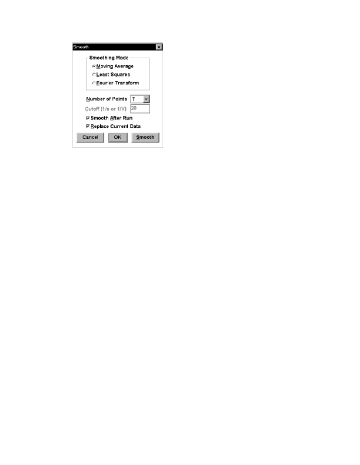
Figure 6-2. Smooth

dialog box.

Smoothing Mode

Point/Cutoff

Smooth After Run

Replace Current Data

Smooth

Cancel

This command exits the dialog box without saving

Default:

This controls the degree of smoothing (higher

When activated, the experimental data is

Moving Average

Point

/lower

Default: 7 (

automatically smoothed at the end of the experiment.

Activating this command will transfer the processed data to main memory

This command activates selected smoothing routine on the data in main memory.

This command exits the dialog box whilst retaining any changes.

any changes.

Cutoff

Point

produces greater smoothing).

Cutoff

), 20 (

)

6.3 Derivative/Integral

These are self-explanatory mathematical operations on the current data of the I-E curves. For differentiation, the 1st, 2nd and 3rd order derivatives are available (Figure 6-3), and are selected using the

Derivative

the Activating the

mode, since differentiation can lead to an increase in the noise level.

Replace Current Data

Order

option. Additional smoothing is available for

transfers the processed data to main memory.

6-3

Page 50

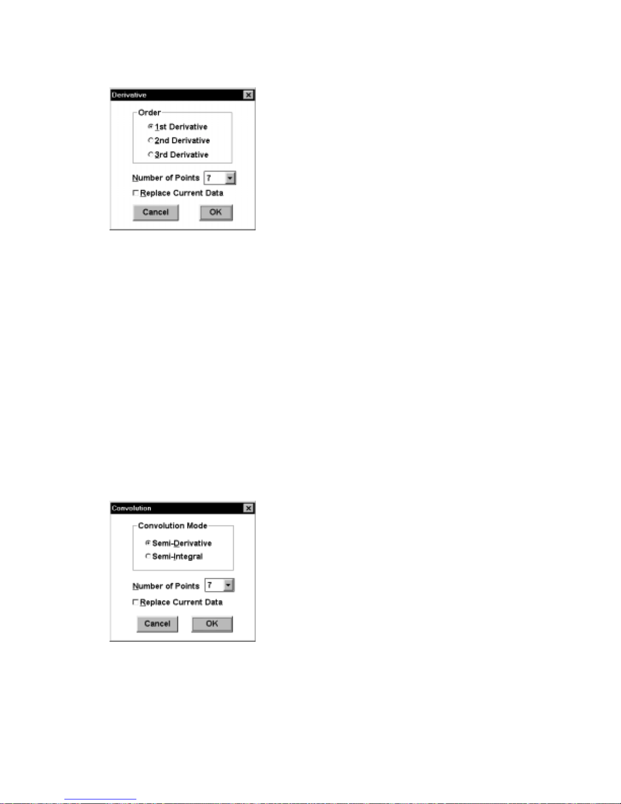
Figure 6-3. Derivative

dialog box.

Differentiation of I is often used for accurate calculation of peak potentials (1st derivative) and half-wave potentials (2nd derivative).

6.4 Convolution

In addition to differentiation and integration, semi-differentiation and semiintegration are also commonly used for processing electrochemical data. Both of these processes are available on the BAS 100W as (Figure 6-4). Additional smoothing is available for semi-differentiation, since this process can increase the noise level. The convoluted data can transferred to main memory us ing

Replace Current Data

. Semi-differentiation is particularly useful for cyclic voltammetry, since it can produce a considerable improvement in the resolution of closely spaced peaks. Semi-integration can be used to remove the effects of iR drop.

Convolution Mode

options

Figure 6-4. Convolution

dialog box.

6-4

Page 51

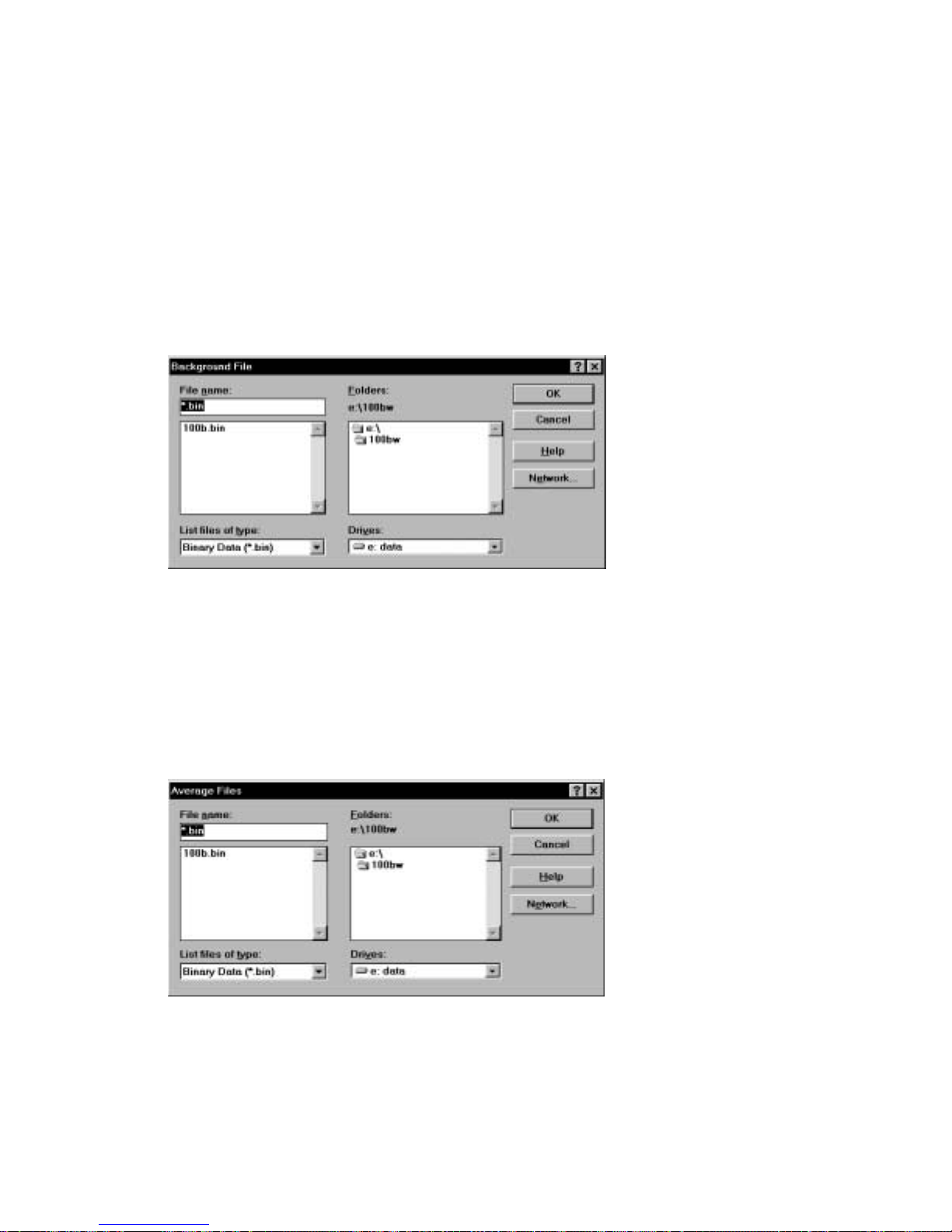
6.5 Background

This command can be used to subtract a voltammogram stored on the hard disk from the voltammogram in the main memory. The data file for subtraction is selected from

Background File

the dialog boxes, see the voltammograms MUST be the same. The subtracted data can be transferred to main memory using

Replace Current Data

dialog box (Figure 6-5) (for a more detailed discussion of file

File

menu section). The potential range of the two

Figure 6-5. Background File

dialog box.

6.6 Average

This command is used to average data files. Up to 100 files can be selected (from the

Average Files

description of file dialog boxes).

Figure 6-6. Average Files

dialog box (Figure 6-6) - see

dialog box.

File

menu section for a more detailed

6-5

Page 52

7. Analysis

7.1 Results Graph

The data available from an electrochemical experiment may be peak potentials and currents, half-wave potentials and limiting currents, slopes and intercepts of straight line plots or the amount of charge passed during the experiments. These data can be obtained using the

Results Graph

There are two options available:

Results Options

windows displays the experimental data, the baseline for peak measurements and the best fit straight line for linear plots (the size and position of this windows can be changed by the user (by dragging the borders or the caption), and are defined initially by the BAS100W.INI file). The The experimental results (see below) are listed in the

CV, LSV

HR (even-numbered segments)

ACV/P, BSWV/P, DPV/P DTACV/P, OSWV

dialog box. When the

, Experimental results - peak potential, current and

Auto

option also selects the appropriate

Selected plot - tailed curve Experimental results - peak potential, current and area

, Selected plot - symmetric curve

area

and

Auto

Manual

. These can be selected from the

option is selected, the

Main

window.

Results Graph

Peak Shape

PSACV/P, TACV/P

BSWSV, DPSV, LSSV OSWSV

HDM, NPV/P, RDE, SCP

CA, CC

, Selected plot - symmetric curve

Experimental results - peak potential, current and area

Selected plot - sigmoidal curve Experimental results - half-wave potential

Selected plot - straight line plots (i vs. t Q vs. t

1/2

for CC)

7-1

1/2

for CA,

Page 53

Experimental results - slope and intercept

(N.B. Due to the finite time required for the potential step to be complete, the data in the first few milliseconds of potential step experiments is often distorted. The BAS 100W

Auto

option therefore only uses the last 80% of the collected

data when calculating slopes and intercepts).

Experimental results - Initial current

End current Current ratio Time Total charge Net charge

LOGI

Selected plot - I vs. E curve Experimental results - minimum potential, log i at the minimum potential

ECM

Experimental results - t

and potential of zero

max

charge

There are no results available for HR (odd-numbered segments),

IMP

and

In addition to the

Results Graph

, the

window also displays the

DPTB, TB, TPTB

coordinates of the mouse cursor as it is moved within the axes. A selected area can be expanded (Zoomed) by dragging the mouse (using the left mouse button) between diagonally opposite corners of the defining rectangle. This operation can be reversed by clicking the left mouse button.

When using the the user. Click and hold down the

Manual

option, the baselines for calculation of results are defined by

right

mouse button at the starting point of the baseline and drag the mouse across the graph to the end point of the baseline. As the mouse is moved within the

Results Graph

window, the coordinates of the mouse cursor are shown in the lower left corner. The number of baselines that must be defined depends on the nature of the plot:

a) Symmetric and tail curves - define one baseline b) Sigmoidal curves - define two baselines c) Straight line plots - define two points on the X axis

For symmetric and tailed plots, the peak area is also listed in the Main window (the peak area is the area between the curve and the user-defined baseline (Figure 7-1)).

7-2

Page 54

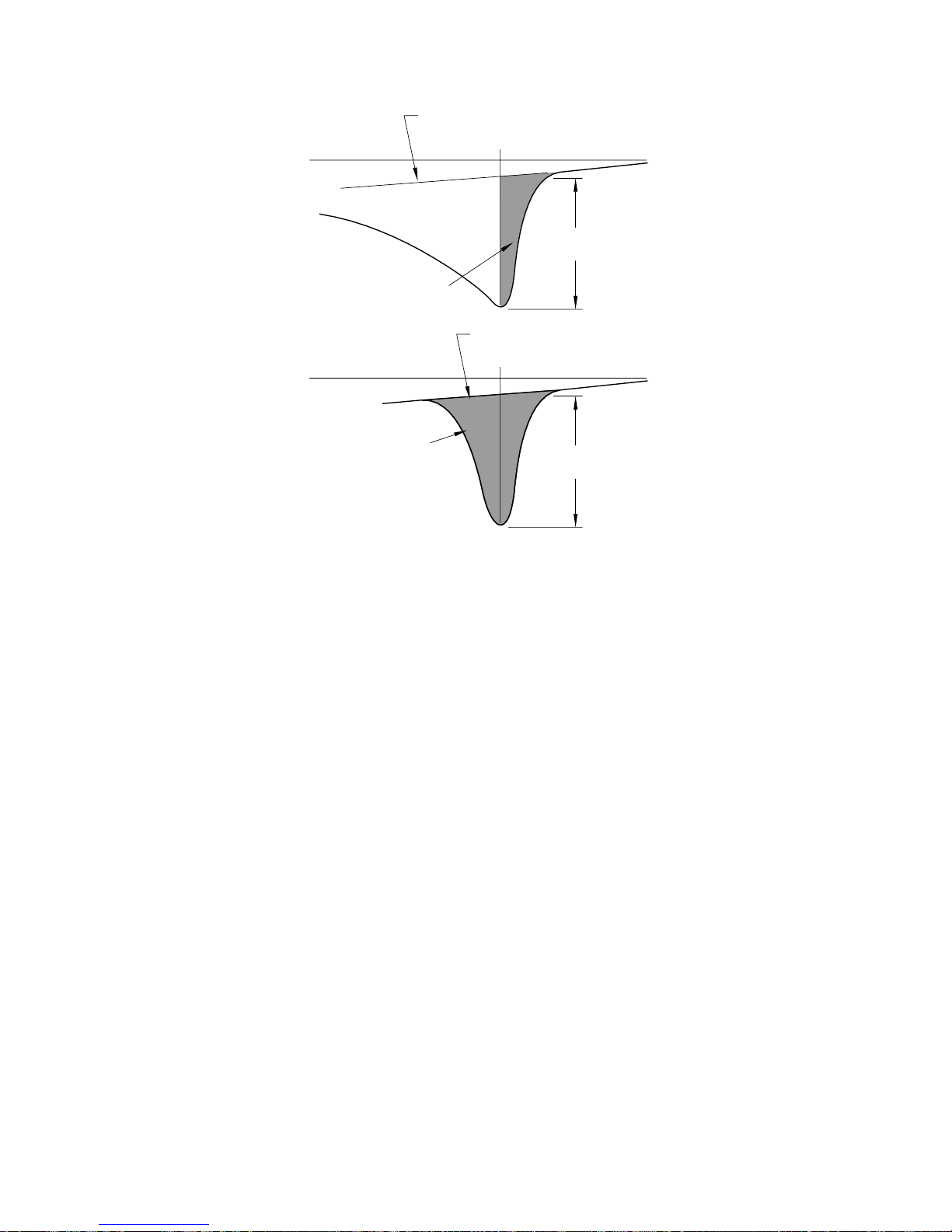
PEAKAREA

BASELINE

PEAK

POTENTIAL

BASELINE

PEAK

POTENTIAL

PEAK

CURRENT

PEAK

CURRENT

Figure 7-1.

Peak area for symmetric and tailed curves.

Determination of Peak Potentials and Inflection Points

NOTE: If there are fewer than 30 points available in a data set of segment, peak finding is not possible and a warning message is shown.

The peak potentials of tailed and symmetric current-potential curves and inflection points of sigmoidal current-potential curves are determined by the manipulation of the first or second derivatives respectively. First derivatives are calculated as differentials across a potential window, ∆E, of about 25 mV; that is,

I is calculated as I(E-25 mV)-I(E). This order is used to produce a consistent

∆

sign convention. The 25 mV interval is not rigid. The actual value is chosen such that an odd number of data points intervene, so that the ∆I value can be assigned to the middle potential of the interval. The derivative plots are actually plots of these ∆I's vs. assigned median ∆E values, not ∆I/∆E vs. ∆E, so the vertical axis has dimensions of current on the same scale used for the ∆I vs. ∆E plot. The derivative values for the first 12 mV and the last 12 mV in a scan are simply equated to the values assigned to the first and last potentials at which ∆I values could be assigned. The second derivative works in the same way, but it operates on the first derivative array.

Peak potentials are determined by examining the first derivative plots. The peak potential value, E

to minus or minus to plus. The first ∆I sign reversal becomes the E

, is determined by first looking for a sign reversal; that is, plus

window (note

7-3

Page 55

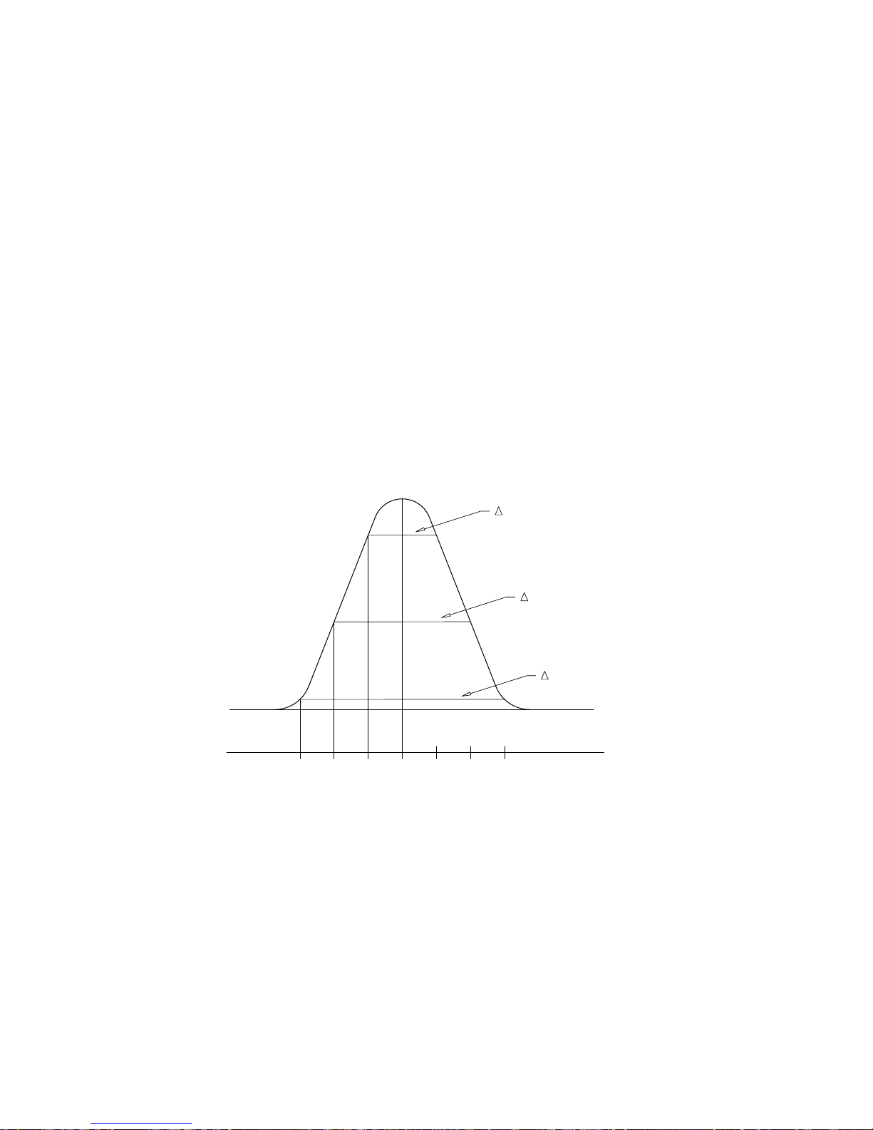
that a 25 mV potential window is being examined for each ∆I calculated). To ensure that it is a true peak (i.e., not merely noise), two criteria must be met. First, the 3 points (∆I values) on either side of the E

window are examined for

continuity of sign; that is, there are three consecutive positive values on the plus side and three consecutive negative values on the minus side. If this test is passed, the actual E

value is determined by choosing the largest current value, I

max

, in a potential window that is 25 mV greater than and less than the median E of the E window.

The second criterion provides a measure of the rate at which the peak is being generated. A rapidly changing peak is more likely to be noise rather than a real electrochemical peak. This noise discrimination routine is implemented by examining the peak width at 50, 100 and 150 mV preceding the peak potential E (Figure 7-). The peak width ratio ∆E50/∆E100, ∆E50/∆E150 and ∆E100/∆E150 are calculated; if these are less than the corresponding values for peak with a

Peak Width

of 200 mV (

Half Peak Width

is the difference between the

Half

potentials at which the current is half the peak current), then the peak is reported

E(peak)

E(50)

E(100)

E(150)

(+) (-)

+50 +100 +150

Figure 7-2.

Peak finding criteria.

Determination of Peak Currents, Limiting Currents and Peak Areas

The most important part of these measurements is the determination of the current baseline. The method for this depends on the curve shape. Peak area is given in units of Amps x Volts. To convert into coulombs, for cyclic voltammetry, the area must be divided by the scan rate (Volts/Sec).

7-4

Page 56

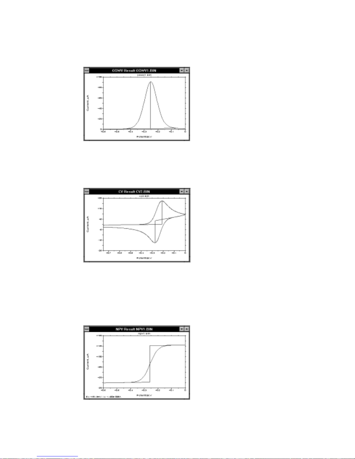
Symmetric

in the range of E

curves - The baseline is the line between the two current minima

+ 250 mV (Figure 73).

Figure 7-3.

Tail

50 mV apart in a range of 250 mV preceding E

Figure 7-4.

Sigmoidal

Symmetric current response.

curves - The baseline is the line between two points on the I vs. E curve

(Figure 7-4).

Tailed current response.

curves - Two baselines are required to measure the limiting current. These are defined by two points on the I vs. E curve 50 mV apart in a range of 250 mV either side of E

(the half-wave potential) (Figure 7-5).

1/2

Different values are chosen to find the lines of absolute minimum slope.

Figure 7-5.

Sigmoidal current response.

7-5

Page 57

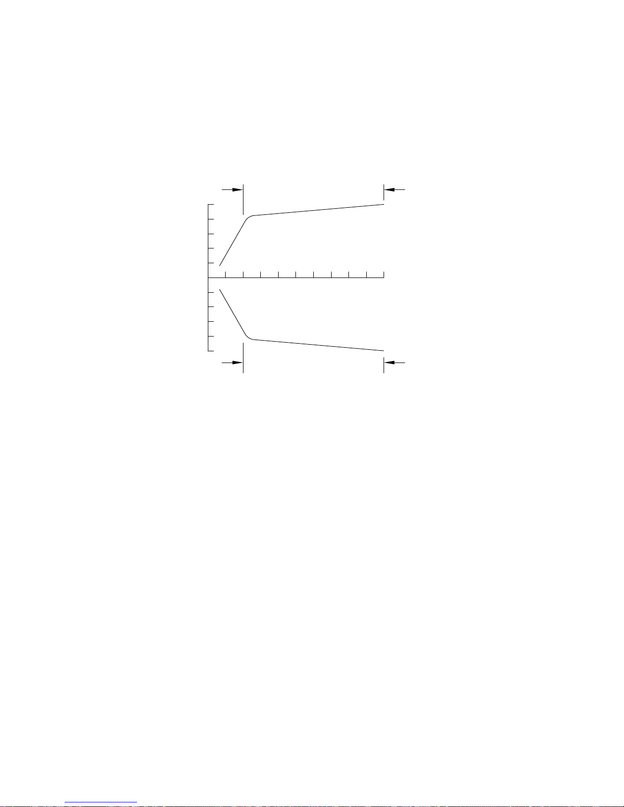
Determination of the Slope and Intercept of an Anson or Cottrell Plot

The slope and intercept of the CA Cottrell plot and the CC Anson plot are determined by an unweighted linear least squares fit routine on the last 80% of the data points following both the forward and reverse potential steps (Figure 7-6).

80% TOTAL NUMBER

FORWARD

STEP

OF DATA POINTS

CHARGE (uC)

REVERSE

STEP

Figure 7-6.

80% TOTAL NUMBER

OF DATA POINTS

Selection of points for the Anson plot.

In all these cases, the lines selected by the

1/2

mSEC 15.8

Auto

screen. These can easily be changed using the calculated slopes are mA

1/2

for Cottrell plot and C/ms

•

option are displayed on the

Manual

option. The units of

1/2

for Anson plot.

7-6

Page 58

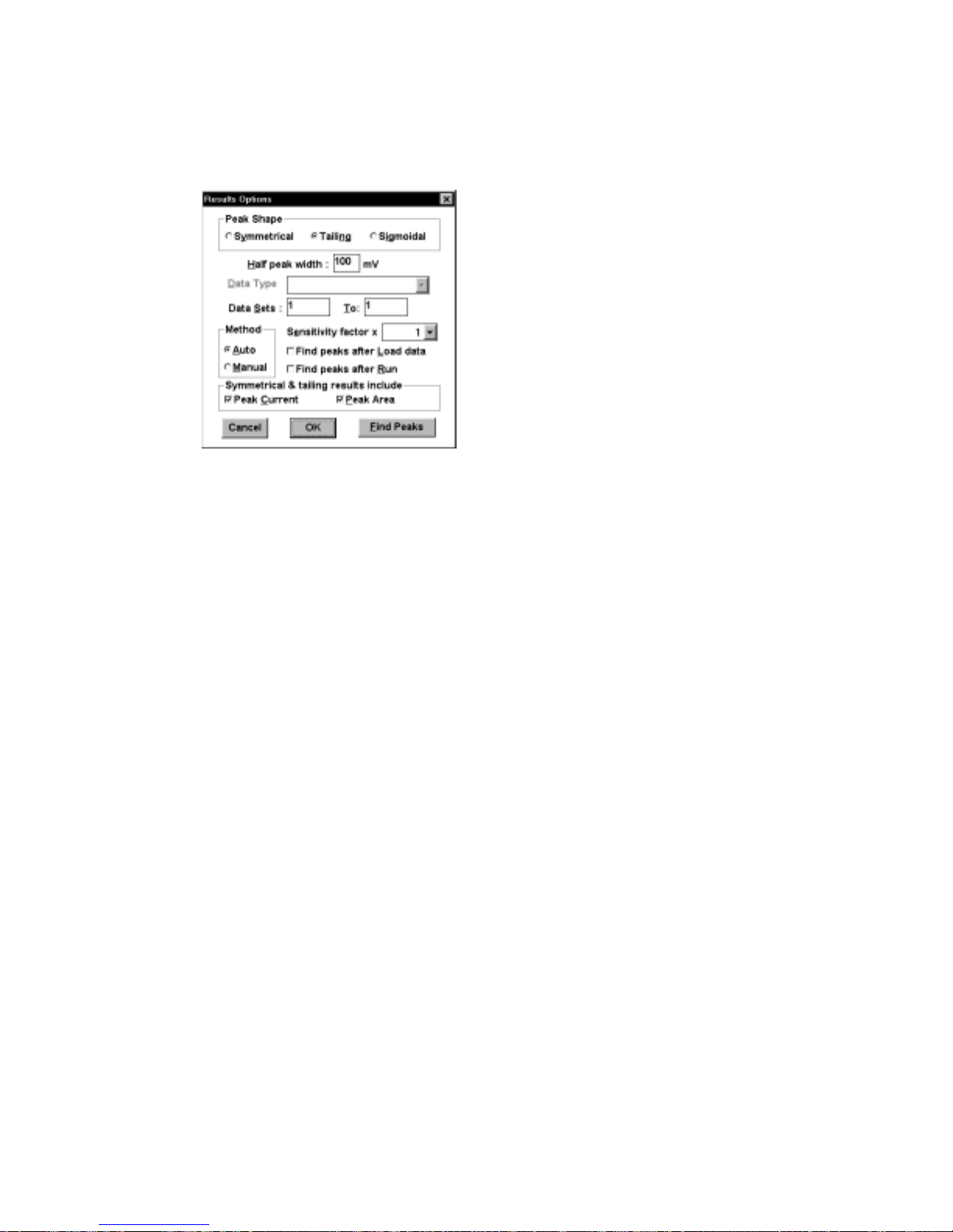
7.2 Results Options

Figure 7-7. Results Options

Peak Shape

Half Peak Width

Data Type

Data Sets

dialog box.

This defines the shape of the curve. There are instances when the default peak shape selection is not appropriate: for example, when using microelectrodes at low scan rates, as this produces a sigmoidal plot for CV.

This defines the expected width of the peak (it may be necessary to increase this value for broader peaks).

This defines how the experimental data is presented when there is more than one presentation format (i.e., BE, CA and CC). The default as follows:

vs. Time

This defines which data set is displayed when there is more than one data set (i.e., CV,

OSWSV Sets

is defined by the

(specified in

OSWSV

number of

Data Sets

The default for CV, the first segment for

Current vs. Time

(for BE and

TPTB

and

TPTB

, and

Data Sets

were defined in

Data Sets

CC)

). For CV, the number of

General Parameters

have

for HR depends on which

are as follows: all segments

(for CA) and

Number of Segments

Data Sets

General Parameters

OSWV, OSWSV

Data Types

HR, OSWV

1 to 3. The

are

Charge

Data

OSWV

and

7-7

Page 59

, and that segment specified for

Display Data Set

General Parameters

(in

TPTB

Method

Sensitivity Factor

Find Peaks after

If this command is activated, the

Load Data

Find Peaks after Run

Symmetrical and Tailing Results Include

This specifies which option (

Auto

Manual

) is to

be used.

This command adjusts the sensitivity of the peak search operation. The height of the smallest detectable peak decreases by a factor of 10 for each stepwise decrease in the

Sensitivity Factor

Results Graph

will be displayed automatically when a data file is loaded (if it is not activated, the

Single Graph

will

be displayed)

If this command is activated, the

Results Graph

will be displayed when the experiment has ended (if it is not activated, the

Single Graph

will be

displayed).

Select whether Peak Current and/or Peak Area are reported in the results.

7-8

Page 60

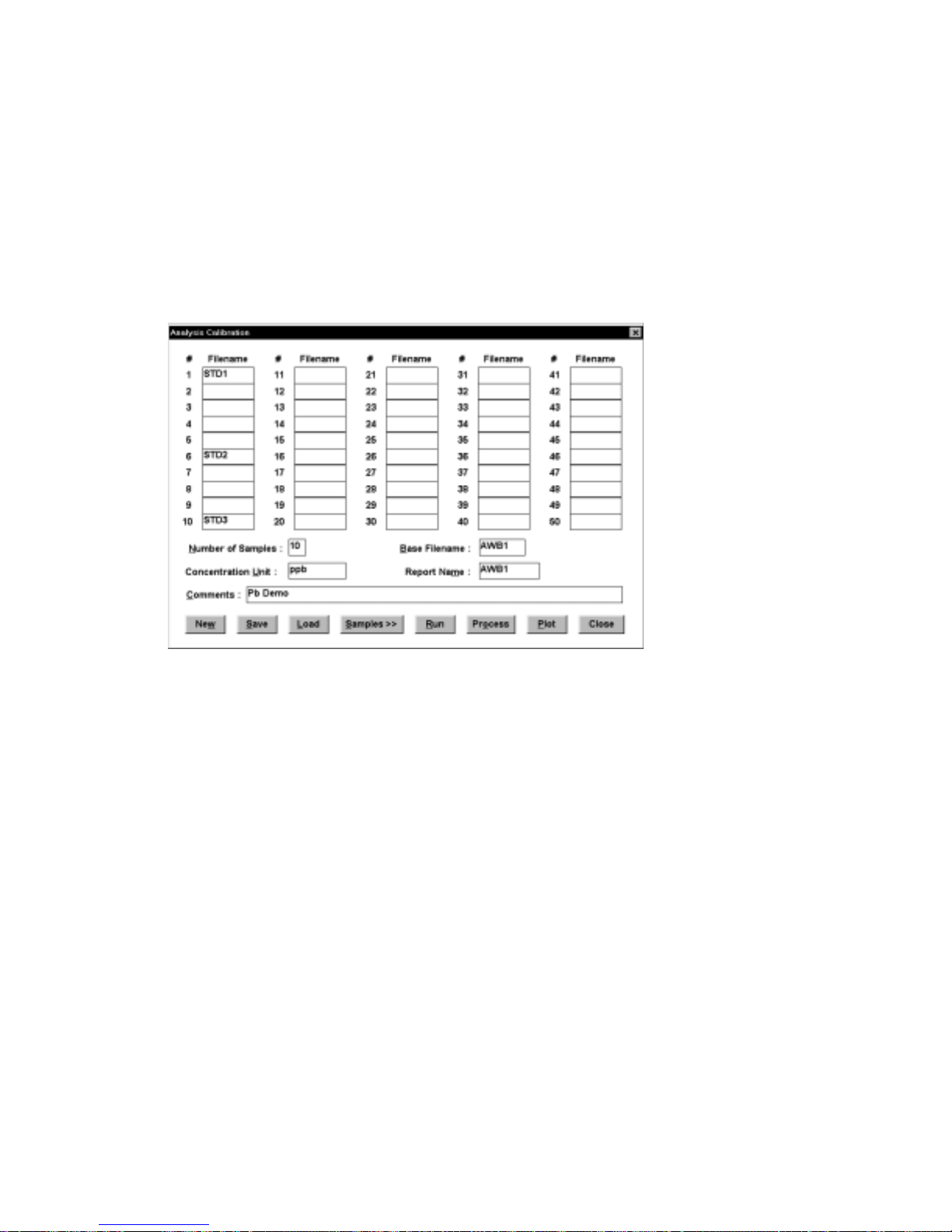
7.3 Calibration

This command is used to set up a calibration curve for quantitative analysis. First, the

Mode

must be selected, and the

General

Specific Parameters

and

entered.

Analysis Calibration

The

8).

Figure 7-8. Analysis Calibration

The maximum sample; if no (e.g., awb11 for sample 1). The specified. In the above example, a total of 10 samples were run, 3 of which were standards - #1, #5 and #10. The reloaded) using the

Number of Samples

Filename

Analysis File

dialog box appears when

dialog box.

is 50. A

is specified, the

Report Name

Analysis

dialog box.

Base Filename

parameters and results can be saved (and

Calibration

Filename

Concentration Unit

and

is clicked (Figure 7-

can be specified for each

+ the sample # will be used

must be

Clicking either an

Conc

with a determined) must also be specified. No information is required for

Prev Analysis Calibration

Samples

Unknown

entration and peak potential (Ep) must been entered for each analyte, together

Tol

erance for Ep. The

and

produces a dialog box which is used to specify each

to move between sample numbers and click

or a

dialog box.

Standard

Number of Peaks

(Figure 7-). For each

(i.e., the number of analytes being

7-9

Escape

Sample

Standard

Unknown

to return to the

, the

s. Use

Page 61

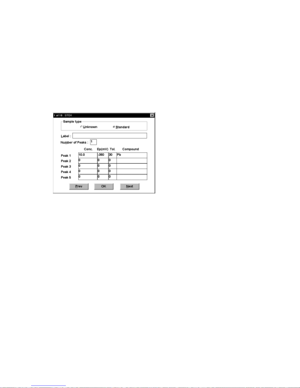
Click request the next sample. When all the samples have been run, the calibration curve for a specified peak can be examined by clicking concentration is saved as a .REP file; the results are also listed in the Main window.

Run

to start the analysis. At the end of each sample run, the software will

Plot

. A report that lists the unknown

Process

peak potentials were used initially). Since 3-digit run numbers are used in the data file names, it may be necessary to rename data files before reprocessing. It should also be noted that the first run number is now 001, not 0 as in previous versions of the BAS 100W software.

Figure 7-9. Samples

is used for reprocessing of existing files (e.g., if incorrect concentrations or

dialog box.

7.4 Standard Addition

This command is used to construct a standard addition curve for quantitative analysis. First, the

The

10).

The

Filename Tol

in the above example, there are three standard additions of 10 ppb. The

Addition

dialog box.

Click the next standard addition. When all the standard additions have been made, the standard addition curve can be examined by clicking

Mode

must be selected, and the

Standard Addition

Number of Peaks, Number of Additions, Concentration Unit

must all be specified. In addition, the peak potentials (Ep) (and

erances) and the total standard concentration after each addition must be entered;

parameters and results can be saved using the

Run

to start the experiment. After each measurement, the software will request

dialog box appears when

General

Specific Parameters

and

Std. Addition

Plot

is clicked (Figure 7-

Standard Addition File

. A report that lists the

entered.

and

Standard

Base

7-10

Page 62

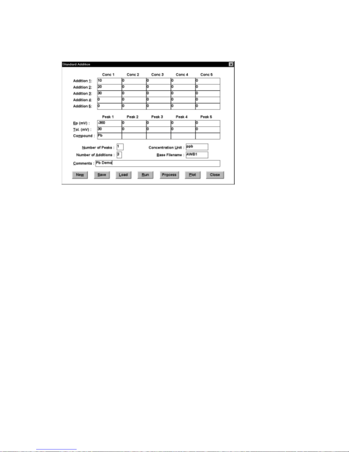
unknown concentration is saved as a .REP file; the results are also listed in the Main window.

Figure 7-10. Standard Addition

Process

is used for reprocessing of existing files (e.g., if incorrect standard additions

dialog box.

or peak potentials were used initially). Since 3-digit run numbers are used in the data filenames, it may be necessary to rename data files before reprocessing. It should also be noted that the first run number is now 001, not 0 as in previous versions of the BAS 100W software.

7-11

Page 63

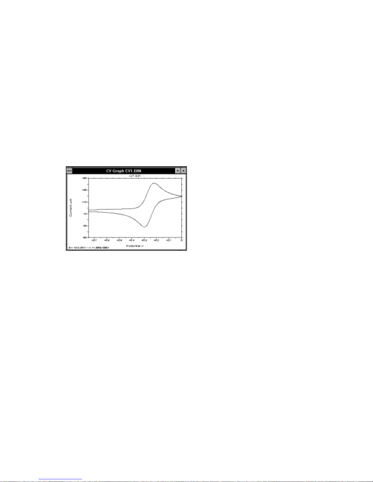
8. Graphics Menu

This Menu is used to display the experimental data after the experimental run and after any post-run data processing.

8.1 Single Graph

Single Graph

The position of this windows can be changed by the user (by dragging the caption or the borders), and are defined initially by the BAS100W.INI file.

window displays the experimental data (Figure 8-1). The size and

Figure 8-1. Single Graph

Single Graph

The experiment and after a data file has been loaded (the

Results Options

to the

In addition to the coordinates of the mouse cursor as it is moved within the axes. Pressing the right mouse button leaves a plus mark on the graph, the coordinates of which are also displayed. A selected area can be expanded (Zoomed) by dragging the mouse between diagonally opposite corners of the defining rectangle. This operation can be reversed by clicking the left mouse button.

Data Type

window.

windows can be displayed automatically at the end of an

Find peaks

dialog box need to be unchecked). The data are graphed according

specified in

Single Graph

Graph Options

, the

Single Graph

, or according to the default

window also displays the

.. check boxes in the

Data Sets

8-1

Page 64

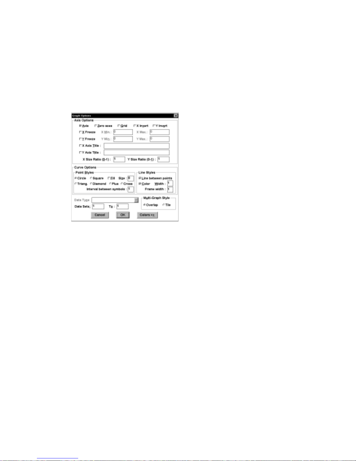
8.2 Graph Options

This dialog box controls the appearance of the graph on the PC screen and on the hard copy (Figure 8-2). All (except particular data file).

X/Y Freeze

and the

Graph Options

Min.

and

Max

are saved in the BAS100W.INI file

. values, which typically only apply to a

Figure 8-2. Graph Options

Axis Options

All the axis options can be enabled or disabled by checking the appropriate box.

Axis

Zero Axes

X/Y Grid

X/Y Invert

X/Y Freeze

When activated, the polarity of the X/Y axis is

When activated, the range of axes is frozen at the

dialog box.

When activated, both axes are drawn.

When activated, dashed lines are drawn on the graph at X=0 and Y=0, if they are within the range of the graph.

When activated, an X/Y grid is displayed.

inverted.

selected range is adjusted automatically to encompass the range of the data set. also applies to graphs displayed during experimental runs. It is a good idea to run the first experiment with

Min

. and

Y Freeze

Max.

values; otherwise, the

Y Freeze

(but not

disabled. After the data

X Freeze

)

8-2

Page 65

for the first run are regraphed with auto-scaling, the

Min

. and

Max.

values are correct for the present

graph.

X/Y Titles

When activated, the specified text replaces the default labels on the axes.

X/Y Size Ratio

This defines the fraction of the total windows area that is occupied by the graph

Curve Options

These control the way the curves are drawn.

Point Styles

Six

Style

s are available in

interior of the

Triangle

symbols can be colored by checking Interval between symbols specifies the interval where dots are replaced by symbols for the data points.

Line Styles

Select

Line between points

with a line of the given draw the points and lines colored pen.

Size

s from 0 to 7. The

Circle, Square, Diamond

to connect the points

Width

, and select

Color

and

Fill

Data Type

Data Sets

This defines how the experimental data is presented when there is more than one presentation format (i.e., BE,

Types

CA, CC

are as follows:

Charge vs. Time

(Nyquist plot) for

(for BE and CC) and

IMP

and

). The default

Current vs. Time

Data

(for CA),

Zi vs. Zr

This defines which data set is displayed when there is more than one data set (i.e., CV,

OSWSV Sets

is defined by the

(specified in

OSWSV

number of

Data Sets

The default for CV, the first segment for

, and that segment specified for

Display Data Set

TPTB

and

). For CV, the number of

General Parameters

TPTB

, and

Data Sets

have

for HR depends on which

were defined in

Data Sets

are as follows: all segments

General Parameters

(in

Number of Segments

Data Sets

General Parameters

OSWV, OSWSV

HR, OSWV

Data

OSWV

1 to 3. The

and

TPTB

8-3

Page 66

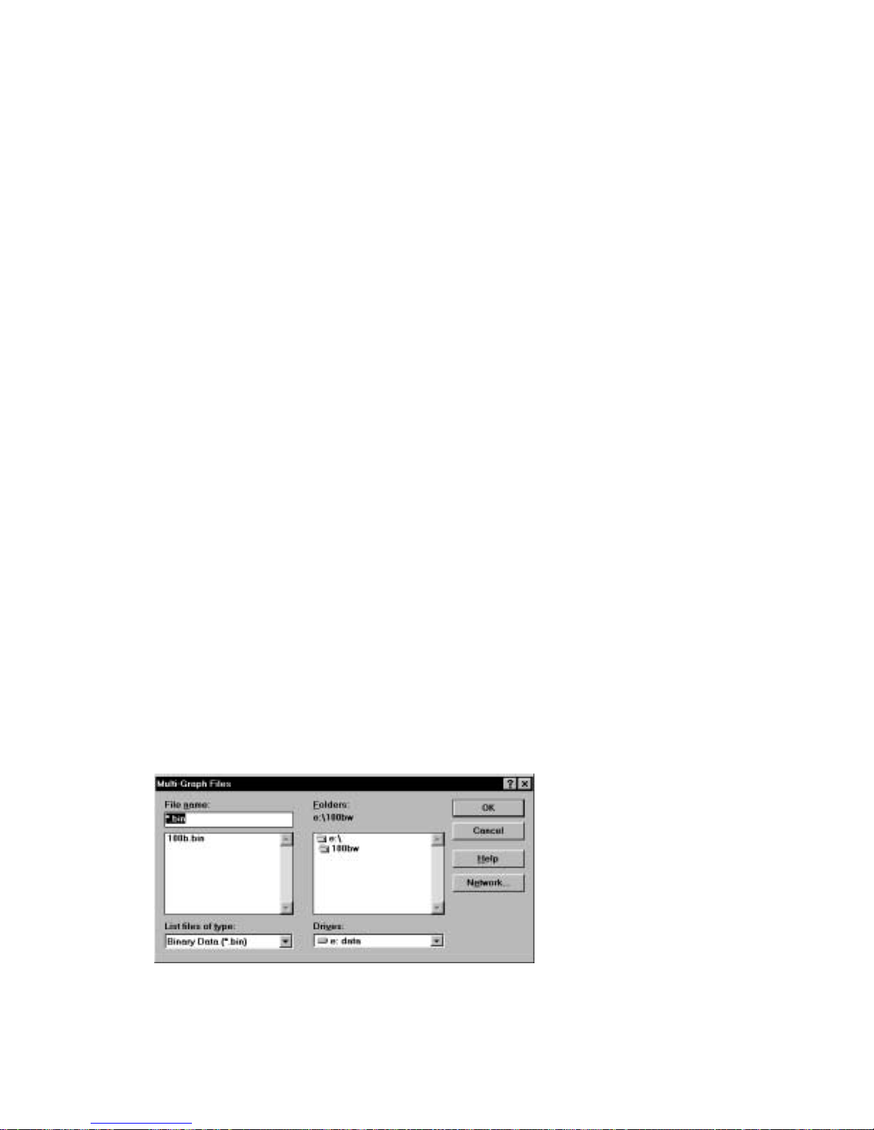
Multi-Graph Style

Overlap

The set of axes and the range of the axes is determined by the data in main memory. The displays each data file on its own set of axes.

option draws all curves on the same

Tile

8.3 Graph Colors

The colors of each feature on the graph can be selected (for both the PC screen and the hard copy). These a color, first click the colored check box beside the selected feature; a cross will replace the color and the sample color patch will change to the present color of that feature. Any color can then be mixed by using the Red, Green and Blue scroll bars or by typing a number between 0 and 255 in the edit box. To apply the present color mix to the selected feature, click the checkmarked box once more. Note that the accuracy of the colors depends the number of colors the display adapter can depict.

Graph Colors

are saved in the BAS 100W.INI file. To change

option

Multi-Graphs

For are used for the first 8 curves, and this sequence repeats for curves 9 through 16, etc.

Default Colors

using the

changes all of the colors back to the original colors.

Overlap

option, the

Curve 1

through

Curve 8

8.4 Multi-Graph

This plots multiple data files, including the data in main memory. The option draws all curves on the same set of axes and the range of the axes is determined by the data in main memory. The own set of axes. Up to 41 files can be displayed, and are selected using the

Graph Files Operation

graph the data. If the data files use different

Data Sets

dialog box (Figure 8-3). If all the data files are for the same

, the

Data Type

and

Data Sets

Data Type

and

are used.

Tile

option displays each data file on its

specified in

Modes of Operation

Graph Options

are used to

, then the default

colors

Overlap

Multi-

Mode of

Figure 8-3.

Multi-Graph Files

dialog box.

8-4

Page 67

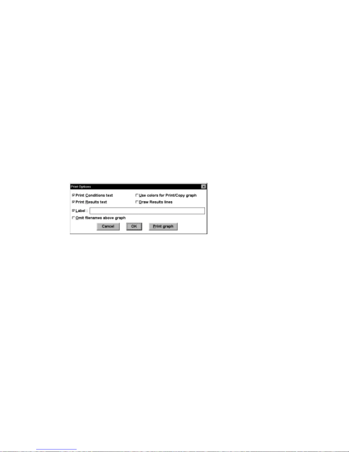
9. Print Menu

9.1 Print Graph

This command transfers the present graph ( default printer (an alternative printer can be selected using options specified in

Print Options

Single Graph

Multi-Graph

Printer Setup

9.2 Print Options

This dialog box contains graph options that pertain only to printed graphs (Figure 9-

1).

Figure 9-1. Print Options

Print Conditions text

dialog box.

This option lists the experimental conditions.

) to the

) using the

Print Results text

Label

Use colors when printing

Draw Results lines

This lists the results from the data analysis.

This is an optional description of the experiment (69 characters maximum).

This option tells the program that the printer in use knows how to translate colors into ink. If it is not checked, everything is printed in black or white. On black-and-white printers, some colors cannot be printed and hence are invisible. In such cases, uncheck this option or try different colors.

This option specifies whether the Results lines (e.g., baselines for peak measurement) are to be drawn on the printed graph (this option also requires the

Results text

9-1

to be active).

Page 68

Omit File Names Above Graph

This option specifies whether the file name is above the graph both on the monitor and on printed/copied to clipboard graphs.

9.3 Multi-Print Files

This command sets up a print queue for data files. Up to 100 files can be selected from the (use the multiple graphs on the same page). If all the data files are for the same

Operation

the data files use different

Type

Multi-Print Files

Multi-Graph

Data Sets

, the

are used.

dialog box. Each data file is printed on a separate page

option in the

Data Type

and

Modes of Operation

Graphics

menu followed by

specified in

, then the default

Graph Options

Print Graph

are printed. If

Data Sets

Mode of

and

9.4 Print Text

for

Data

Print Text

desired lines in the

prints any text selected (highlighted) by dragging the mouse over the

Main

window.

9.5 Copy Text

This command copies to the the mouse over the desired lines in the transferred to other Windows programs.

Clipboard

any text selected (highlighted) by dragging

Main

window. From the

Clipboard

, it can be

9.6 Copy Graph

Copy Graph

From the

Clipboard

transfer the present graph window (without its frame) to the

it can be transferred to other Windows programs.

Clipboard

9.7 Print Setup

This command allows the default printer and other printer options to be changed without using the and the printer driver installed in Windows.

Control Panel

. The options available depend on the type of printer

9-2

Page 69

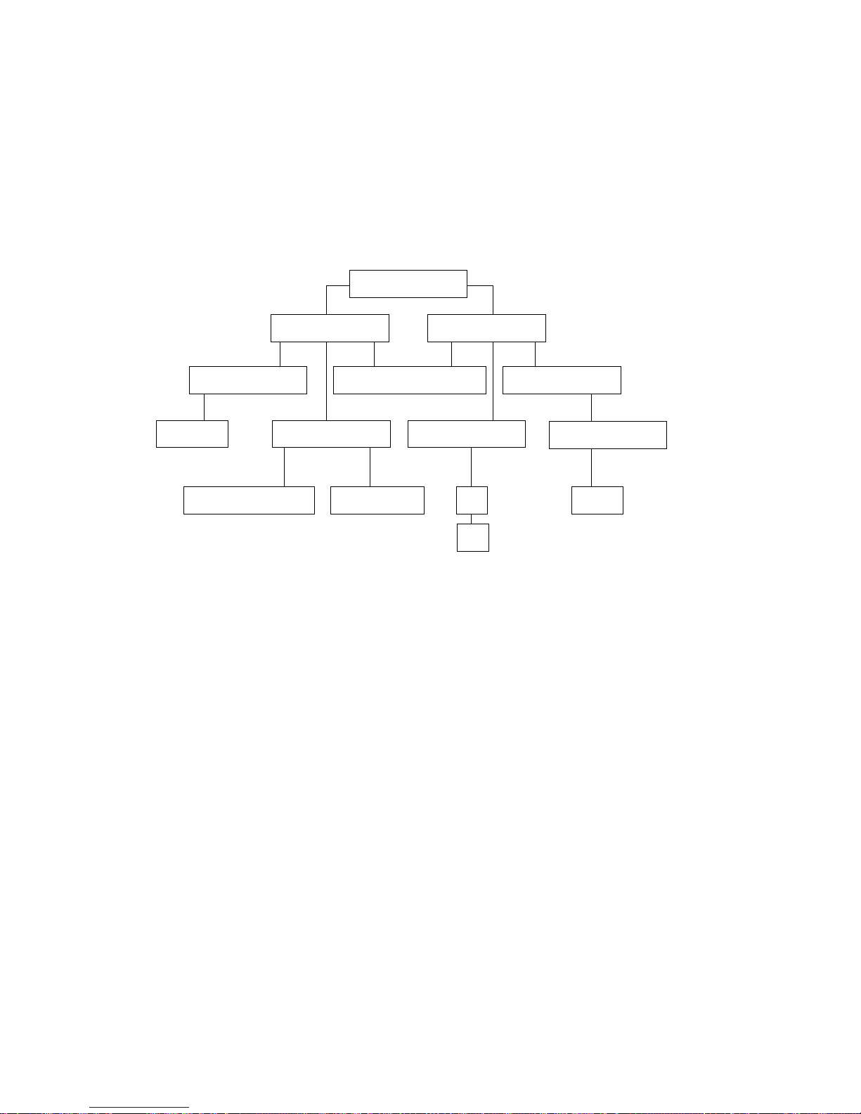
10. Operation Modes

There are 38 techniques available on the BAS 100B/W. This may appear to be a bewildering number, but many of these techniques are related, or are variations of other techniques. There are a number of broad divisions that can be made.

Control Potential

Hydrodynamic

RDE, HDM

Small Amp

ACV, PSACV, SHACV

Voltammetry

(I vs. E)

Pulse Voltammetry

(DPV, SWV, NPV, SCP

Stationary Soln. Stationary Soln.

Large Amp

CV, LSV

Chronoamperometry

(I vs. t at fixed E)

,...)

Hydrodynamic

Control Potential

Electrolysis

LC/EC

a) Voltammetry vs. chronoamperometry (potential step). In voltammetry, the potential is

varied in a defined manner, and the current response is monitored. In chronoamperometry, the potential is held at a fixed value (or is stepped between two values) and the current response is monitored as a function of time.

b) Stationary solution vs. Hydrodynamic. This determines the rate at which electroactive

molecules are brought to the surface of the working electrode (i.e., the rate of mass transport). In stationary solutions, the only mode of mass transport is diffusion, whereas in hydrodynamic techniques, there is a combination of convection (e.g., stirring) and diffusion. Therefore, in these latter techniques, the rate of mass transport can be controlled.

There is another set of techniques (pulse techniques) in which the applied potential is a combination of voltammetry and potential step. This are discussed in more detail below.

Sweep Techniques

(Stationary Solution) Cyclic Voltammetry (CV) Linear Sweep Voltammetry ( Linear Sweep Voltammetry with Log output ( Cyclic waveform (

Step Techniques

CYCLE

(Stationary Solution)

)

LSV

)

LOGI

10-1

)

Page 70

Chronocoulometry (CC) Chronoamperometry (CA) Step waveform (

STEP

)

Pulse Techniques

Differential Pulse Voltammetry/Polarography ( Normal Pulse Voltammetry/Polarography ( Sampled Current Polarography (

Square Wave Techniques

Barker Square Wave Voltammetry/Polarography ( Osteryoung Square Wave Voltammetry (

AC Techniques

Alternating Current Voltammetry/Polarography ( Phase Selective Alternating Current Voltammetry/Polarography ( Second Harmonic Alternating Current Voltammetry/Polarography ( Triangular wave Alternating Current Voltammetry/Polarography (

(Stationary Solution)

SCP

(Stationary Solution)

)

NPV/P

OSWV

DPV/P

)

BSWP/V

)

ACV/P

)

PSACV/P

SHACV/P

TACV/P

)

Differential Triangular wave Alternating Current Voltammetry/Polarography

DTACV/P

(

)

Stripping Techniques

Barker Square Wave Stripping Voltammetry ( Differential Pulse Stripping Voltammetry ( Linear Sweep Stripping Voltammetry (

LSSV

Osteryoung Square Wave Stripping Voltammetry (

BSWSV

DPSV

)

OSWSV

)

Hydrodynamic Techniques

Rotating Disk Electrode ( Hydrodynamic Modulation (

RDE

HDM

)

Time Base

Time Base (TB)

TPTB

DPTB

)

Differential Pulse Time Base ( Triple Pulse Time Base (

Miscellaneous

Bulk Electrolysis with Coulometry (BE) Electrocapillary Measurement (

ECM

) Programmable potential waveform - Hold/Ramp/Step (HR) A.C. Impedance (

IMP

)

10-2

Page 71

There are a number of parameters that are common to all techniques.

a) Potential range. When only a single potential is required, this is defined by

If a potential range is required, this is defined by sweep/scan/step experiments), or

Initial E, High E

Initial E

and

Low E

Final E

and

(for two or more

Initial E

(for single

sweep/ scans/steps in the experiment). The range for any potential is -3276 to +3276 mV.

Sensitivity

techniques (except CC,

. This is the gain of the current-to-voltage converter output. For all

IMP

and

LOGI

), the range of sensitivities is 100 mA/V to 10 pA/V, although for sensitivities greater than 100 nA/V, the Low Current Module (LCM) must be used.

Quiet Time

. This is the time between the initiation of the

potential scan/step. The working electrode is connected at

Run

and the start of the

Initial E

during this time, so that equilibration can occur before the start of the experiment. The allowed range for the

Quiet Time

is 0 to 65535 seconds.

10-3

Page 72

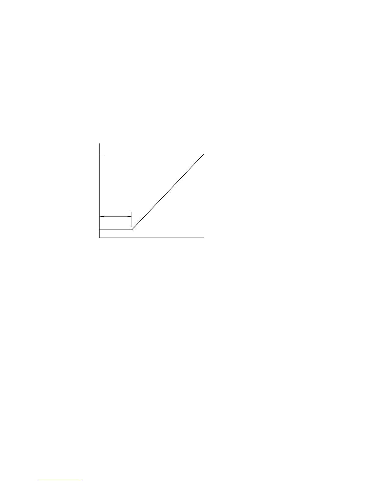
10.1 Linear Sweep Techniques (LSV, CV, LOGI, CYCLE)

LSV

In potential (

, the potential is varied linearly from an initial potential (

Final E

) at a constant rate (

Scan Rate

), and the current is monitored as a

function of the applied potential. The potential wave form for

Initial E

LSV

is shown in

) to a final

Figure 10-1.

FINAL

QUIET TIME

INIT

Figure 10-1.

Potential wave form for

A more commonly used variation of

LSV

is CV. In this technique, when the final potential is reached, the scan direction is reversed and the same potential range is swept again in the opposite direction. Therefore, the product of the electrochemical reaction on the forward scan can be examined on the reverse scan. This feature is one of the main reasons for the widespread use of this technique.

In CV, the potential can be cycled over the same range many times. Three potential parameters are required; the initial potential ( potentials (i.e., the potential at which the direction of the scan is reversed),

Low E

and

. The potential wave form for CV is shown in Figure 10-2.

The simplest I-E curve for CV is shown in Figure 10-3. The asymmetry of the curve is due to the diffusional mass transport. However, there are many other parameters that can affect the shape of this curve; for example, slow heterogeneous transfer kinetics, instability of the oxidized or reduced species, and adsorption. If the heterogeneous electron transfer is rapid (relative to the timescale of the experiment) and both the oxidized and reduced species are stable (again, on the timescale of the experiment),then the redox process is said to be electrochemically reversible. The standard redox potential is the mean of the two peak potentials (E

10-4

Initial E

), and the two switching

High E

and Epc), and the

Page 73

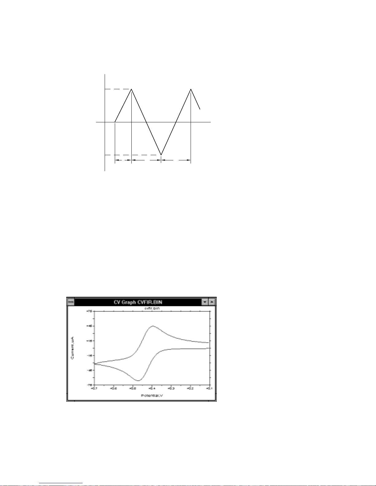
separation of the peak potentials is 57/n mV (n = number of electrons transferred per molecule).

HIGH

INITIAL

LOW E

Figure 10-2.

-E

Potential wave form for

SCAN SEGMENTS

CV.

The peak current for a reversible process is given by the Randles-Sevcik equation:

−

532 12 12

ixnADC

26910

where: i

///

= peak current (A)

n = number of electrons transferred per molecule

A = electrode surface area (cm D = diffusion coefficient (cm C = concentration (mol/cm

= scan rate (V/s)

)

/s)

)

Figure 10-3.

Typical current response for

10-5

Page 74

Therefore, for a reversible process, ip is proportional to the concentration, C, and the square root of the scan rate,

1/2

As discussed above, there are many parameters that can affect the shape of the

curve. Slow electron transfer kinetics can increase the separation of the peak potentials (∆E examining the variation of ∆E between the working and reference electrodes can also increase ∆E

), and the rate constant for electron transfer can be calculated by

with scan rate. However, uncompensated resistance

. The effect of

uncompensated resistance can be lowered or eliminated using electronic iR compensation (see

iR Compensation

under the

Control

menu).

Another application for CV is the study of the reactions of electrolyzed species. These are generated on the forward scan, and their reactivity can be examined on the reverse and subsequent scans. Qualitative estimates of reaction rates can be obtained by varying the scan rates.

The simplicity and speed of CV means that it is often used as the first technique to characterize a redox system, and it is a very powerful technique for qualitative analysis of kinetics and mechanism. However, quantitative kinetic measurements using CV generally require digital simulation, since there is no other way to separate the effects of slow electron transfer and chemical reactivity.

The charging current that is present in CV and techniques for quantitative analysis. However,

LSV

limit their usefulness as

LSV

is used as one of the techniques for the detection of trace metals using stripping voltammetry. This is discussed in more detail in section 10.6.

It is important to note that the potential wave form used for CV and

LSV

on the BAS 100B/W (and other digital instruments) is a staircase wave form, since it is impossible to generate digitally a true linear wave form. There has been much discussion on the equivalence of "digital staircase" CV and

LSV

and

, and it has been shown that variation of the parameters used for the

LSV

and "analog"

"staircase" techniques can lead to significant differences. Theoretical studies have shown that equivalence can only be guaranteed if the potential step height of the staircase wave form is less than 0.3/n mV (where n = number of electrons transferred). Therefore, for BAS 100B/W for CV and the step height is 0.1 mV. However, for

Scan Rates

LSV

is identical to a true analog linear wave form, since

in mV/s, the potential wave form used on the

Scan Rates

in V/s, the step height is 1.6 mV,

so small inequivalences may arise.

BAS has a considerable number CV Notes, together with articles and Capsules that describe the applications of CV (the articles and capsules are listed below). These can beobtained at no charge from BAS.

10-6

Page 75

BAS Capsules

132 Adsorption of Reduced Glutathione on a Mercury Surface 141 Determination of Heterogeneous Electron Transfer Rate Constant 264 Electrochemical Conversion of [FeIr

(CO)16]- to [FeIr5(CO)15]

265 Identification of the Products of Oxidation of [CpFe(CO)2]2 Using Infra-

red Spectroelectrochemistry

266 Potentiostatic Measurements of a Tc(III)/Tc(II) Couple Using an OTTLE

Cell 267 Cis-Trans Isomerization of Ru(MeOCS 271 Two Electron Reduction of [CpCo(NO)] 272 Reductive Dimerization of CpW(NO)I

2)2

(PPh3)

273 Investigation of Electron Transfer Chain Catalysis Using Cyclic

Voltammetry 274 Calculation of the Standard Heterogeneous Charge Transfer Rate Constant

) for Dimeric Iron Fulvalene Complexes Using Cyclic Voltammetry

275 Investigation of E-Z Isomerization of Iron Alkenyl Complexes Using

Semi-Derivative Voltammetry 276 Investigation of the Metal-Initiated Oligomerization of Alkynes

Current Separation Articles

1 Voltammetry Primer: Basic CV, R.E. Shoup, 4 (1982) 31. 2 Cyclic Voltammetry as a Tool for Assessing Dual Electrode Detector

Feasibility, R.E. Shoup, 4 (1982) 48. 3 Electrochemistry for the Nonelectrochemist, P.T. Kissinger, 6 (1985) 62. 4 Voltammetric Microelectrodes, J.O. Howell, 8 (1987) 2. 5 Cyclic Voltammetry: The Electrochemical Equivalent of Spectroscopy,

W.R. Heineman and P.T. Kissinger, 9 (1989)15. 6 Doing Things by Halves: Semidifferentiation in Voltammetry, K. Oldham

and R. Philp, 10 (1990) 3. 7 The Electrochemical Behavior of Nifedipine and Related Compounds and

Quantitation of Nifedipine in Plasma by LCEC, K. Bratin and P.T.

Kissinger, 4 (1982) 4. 8 Reduction of Anthracyclines at a Glassy Carbon Electrode, J. Pursley, 4

(1982) 11. 9 Electrochemical Characterization of Ni/Ni

Fe(CN)

, K. Kuo, 5 (1983)

30.

10 Electrochemical Characterization of Battery Electrodes, K. Kuo, 5 (1983)

45.

11 Chromatographic and Electrochemical Investigation of Codeine, D.A.

Meinsma and P.T. Kissinger, 6 (1985) 42. 12 Electrochemical Oxidation of Caffeic Acid: Formation of 6,7-

Dihydroxycoumarin, T.M. Kenyhercz and P.T. Kissinger, 6 (1985) 48. 13 Cyclic Voltammetric Studies of Transition Metal Complexes, K.A.

Connor and R.A. Walton, 6 (1985) 67.

10-7

Page 76

14 Transient Electrochemical Response of Thermal Ruthenium Oxide Thin

Films in Aqueous Electrolytes, E.W. Tsai, P. Abraham and K. Rajeshwar,

9 (1990) 130. 15 Electrochemistry of C60 and C70 Fullerenes, A.W. Bott, 10 (1991) 137. 16 Cyclic Voltammetry in Organometallic Chemistry, A.W. Bott, 10 (1991)

139.

17 Analysis of the Isomerization of Cr(CO)

PPh2) Using Cyclic Voltammetry Simulation, A.W. Bott, 13

2CH2

(

-Ph2PCH2CH2P(Ph)

(1994) 45. 18 Electron-Transfer-Induced Isomerization of (Cyclooctatetraenecyclo

pentadienyl-cobalt, A.W. Bott, 13 (1994) 49. 19 Electrochemical Deligation of Bis(arene)iron(II) Dications, A.W. Bott, 13

(1994) 70.

The potential waveform for

LOGI

is the same as that for

LSV

. For

LOGI

, the output is the logarithm of the absolute value of the current output. This can linearize portions of the voltammogram where the current is controlled only by the rate of electron transfer. Such plots are called Tafel plots, and are used to obtain transfer coefficients and exchange currents. These are frequently used in corrosion studies (to measure the corrosion (exchange) current). The log plot can also be used to display a large current range in a single plot.

CYCLE

has the same waveform as CV. However, in

CYCLE

there is no digital data acquisition, but the analog current-to-voltage converter is connected and the output is sent to the I

jack on the back panel of the BAS 100B. This is used when many CV

OUT

cycles are required, and the required data storage exceeds the data storage capacity. It can also be used to condition the working electrode.

Mode = LSV

General Parameters

Initial E (mV) = 0 -3276 to 3276 Final E (mV) = 0 -3276 to 3276 Scan rate = 100 mV/s 1 to 51200 (µV/s)

1 to 51200 (mV/s) 1 to 300 (V/s)

Sensitivity = 1 µA/V 100 mA/V to 100 nA/V (10 pA/V with the

Low Current Module)

Specific Parameters

Sample Interval (mV) = 1 1 to 20 Quiet Time (sec) = 2 0 to 65535

10-8

Page 77

Mode = CV

General Parameters

Initial E (mV) = 0 -3276 to 3276 High E (mV) = 0 -3276 to 3276 Low E (mV) = 0 -3276 to 3276 Scan Rate = 100 1 to 51200 (µV/s)

1 to 51200 (mV/s)

1 to 300 (V/s) Initial Direction = Negative Negative or Positive Number of Segments = 2 0 to 65535 Sensitivity = 1 µA/V 100 mA/V to 100 nA/V (10 pA/V with the

Low Current Module)

Specific Parameters

Sample Interval (mV) = 1 1 to 20 Quiet Time (sec) = 2 0 to 65535

Comments (LSV/CV

)

a) The wave form generator that drives the potentiostat is a Digital-to-Analog

Converter (DAC) with 2

(65,636) resolution elements. The resolution of the

staircase potential wave form is 0.1 mV, which generates a potential range of

3276 mV. The rate at which the potential can change (the

Scan Rate

) is

dependent on the rate at which each digital element can be changed. This rate is determined by the speed of the clock pulses, which is set at 2.048 x 10

pulses/s in the BAS 100B/W. The rate of change from the DAC is controlled by allowing only a fraction of the clock pulses to reach the DAC. The allowed

Scan Rates

(for mV/s) are calculated from the equation shown below and some values are listed in Table 10-1. If the entered scan rate is between two values, the higher scan rate will be used.

2.048 x 10

pulses/s x 0.1 mV/pulse =

Scan Rate

(mV/s)

Frequency divisor

10-9

Page 78

Frequency divider Scan Rate (mV/s) Frequency divider Scan Rate (mV/s)

4 51200 200 1024 5 40960 201 1019 6 34166 202 1014 7 29257 203 1009 8 25600 204 1004

9 22755 205 999 10 20480 206 994 11 18618 207 989 12 17066 208 984 13 15753 209 980 14 14628 210 975

15 13653 .. ..

16 12800 .. ..

17 12047 500 410 18 11378 501 409 19 10799 502 408 20 10240 503 407

21 9752 .. ..

22 9309 (1 mV/s resolution)

Table 10-1.

For

Scan Rates

Frequency divider Scan Rate (mV/s) Frequency divider Scan Rate (mV/s)

10 327 31 105 11 297 32 102 12 273 33 99 13 252 34 96 14 234 35 93 15 218 36 91 16 204 37 88

17 192 .. ..

18 182 .. ..

19 172 .. ..

20 613 40 81 21 156 41 79 22 148 42 78 23 142 43 76

24 136 .. ..

25 131 .. ..

26 126 60 54 27 121 61 53 28 117 62 52 29 112 30 109 80 40

Table 10-2

Some allowed

Scan Rates

for this resolution are shown in Table 10-2.

Some allowed

Scan Rates

for mV/s.

of V/s, the resolution of the staircse is 1.6 mV. A list of some

Scan Rates

for V/s.

10-10

Page 79

b) The

Sample Interval

(potential resolution) is dependent on the

The best potential resolution for the

Scan Rates

Scan Rate

(for mV/s) are shown below.

Scan Rate (ν)/mV/s

ν ≤

15753 17066 ≤ ν ≤ 29257 34166 ≤ ν≤ 40960

= 51200

Resolution/m

1 2 3 4

c) The maximum number of data points that can be collected in one experiment

is 8000. Therefore, a

Sample Interval

of greater than 1 mV may be required for multisegment experiments. Any such changes are made automatically by the software.

d) When the

performed. If

Number of Segments

Initial E

is between

is 0, one complete potential cycle is

High E

and

Low E

, start at

Initial E

sweep to one switching potential, reverse and sweep to the other switching potential, reverse and return to the

High E Segments

e) The maximum

Low E

= 2.

, then

Number of Segments

Initial E

is determined by the data storage

capacity, and hence depends on the potential range,

Initial E

. If

is the same as either

= 0 is the same as

Sample Interval

Number of

, etc.

Graphics Menu (LSV

Single Graph

Analysis Menu (LSV

Auto

The

option for

and the peak potentials and peak currents are listed in the

and CV)

displays the current vs. potential plot.

and CV)

Results Graph

displays the current vs. potential plot,

Main

window for

all the segments scanned. Alternative baselines can be set by the user through

Manual

the

Math Menu (LSV

option.

and CV)

The derivative voltammogram is sometimes used to measure the peak potential more accurately, since the sign of the first derivative change at the peak potential. The convoluted voltammograms (both semi-derivative and semi-integral) are sometimes reported. The semi-differential voltammogram has symmetric peaks and better resolution than the standard voltammogram (see BAS Capsule 275 and Current Separation article 6. The semi-integral is used to correct for iR drop.

10-11

Page 80

Mode = LOGI

The

General

Specific Parameters

and

for

LOGI

are the same as for

with two exceptions.

Scan Rates

generally used for

are only allowed in µV/S, since very slow scan rates are

LOGI

experiments. The range for

Scan Rate

51200.

b) The default

Sensitivity

is set to Auto; that is, automatic current ranging. This is used because of the wide range of current values generally measured in

LOGI

experiments.

Graphics Menu

Single Graph

displays the log (absolute current) vs. potential plot.

Analysis Menu

The

Auto

option for

Results Graph

displays the log (absolute current) vs. potential plot and the minimum potential (Min E) and the log I at this potential are listed in the

Main

window.

LSV

is 1 to

Tafel slopes and intercepts can be measured using the

Manual

option. The user must define the slope of the line by specifying two X values on the plot. In addition, the axis for the intercept must be defined (by clicking any point along this axis). This axis is generally the line E = Emin.

Mode = CYCLE

General

The

, except that there is no data acquisition or handling parameters. The

Specific Parameters

and

for

CYCLE

are the same as those for

analog-to-digital conversion function is disabled, but the analog current-tovoltage converter is connected, and the output is sent to the Iout jack on the rear panel of the BAS 100B. If the current is not being recorded, it is advisable to adjust the current is being recorded (e.g., on an XY recorder), the

Sensitivity

to 100 mA/V to avoid saturation. If the

Sensitivity

adjusted appropriately.

must be

10-12

Page 81

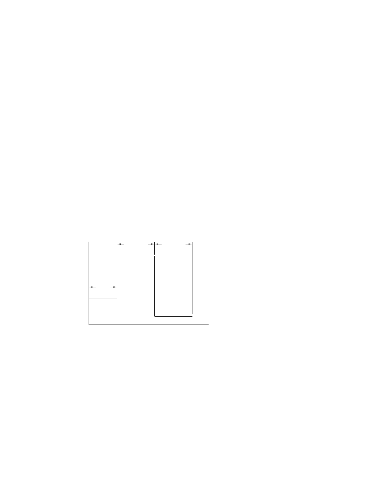
10.2 Potential Step Techniques (CA, CC, STEP)

In these techniques, the potential is stepped from one value to another, and the current (CA) (or charge (CC)) response is monitored as a function of time (it should be remembered that charge is simply the integral of current). After the potential has been held at this value for a time τ, the potential can be stepped to another value (often the original potential). Therefore, potential step experiments can be single step, or double step.

General Parameters

The potential (

Initial E

), and high and low potentials ( The potential can be stepped from determined by the

Pulse Width

(the

High E

Initial Direction

), the potential can be stepped in the opposite direction (from

High E

For CC, the only potentials are the initial potential (

Final E

(

) (Figure 10-5).

are slightly different for CA and CC. For CA, an initial

Low E

High E

Initial E

Positive

to either

Negative

Low E

), and is held at this value for time τ (Figure 10-4).

Initial E

Low E

and

) are required.

High E

(this is

respectively). After time

) and the final potential

Low

HIGH E

INIT. E

LOW E

Figure 10-4.

QUIET

TIME

Potential wave form for

PULSE WIDTH

The current/charge response depends on the values of the initial and final potentials. If no faradaic reaction occurs at either potential (a faradaic reaction is the electrolysis of any molecules in solution), then the response is due to charging of the electrode (the charging or background current). The response is a current 'spike', which decays exponentially.

10-13

Page 82

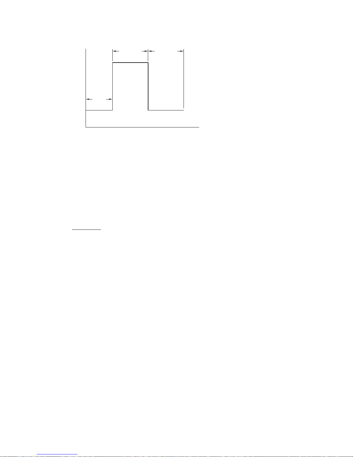
FINAL E

INIT. E

QUIET

TIME

PULSE WIDTH

Figure 10-5.

Potential wave form for

Often, the initial potential is a potential at which no faradaic reaction occurs, and the final potential is a potential at which the Faradaic reaction occurs very rapidly; that is, the electroactive molecules are electrolyzed as soon as they arrive at the surface of the working electrode. The current is therefore determined by the rate of mass transport from the bulk solution to the surface of the working electrode; that is, the rate of diffusion. The diffusion controlled current is given by the Cottrell equation.

12 12

nFAD C

where: i = current (A)

n = number of electrons transferred per molecule F = Faraday`s constant (96,485 C/eq)

A = electrode area (cm D = diffusion coefficient (cm C = concentration (mol/cm

)

/s)

)

t = time (s)

The diffusion controlled faradaic current therefore decays with t chronoamperogram is shown in Figure 10-6). The analogous expression for the diffusion controlled charge (Q

1/2

proportional to t

), and a typical chronocoulogram is shown in Figure 10-7.

Although i (or Q) vs. t plot is displayed during the experimental run, it is also useful to plot i vs. t

-1/2

(for CA) and Q vs. t these are straight line plots, and are often referred to as the Cottrell plot (for CA) and the Anson plot (for CC). These plots are available as standard plots on the BAS 100B/W.

-1/2

(a typical

) is the integral of the above expression (i.e., Q

diff

1/2

(for CC). For diffusion controlled systems,

10-14

diff

Page 83

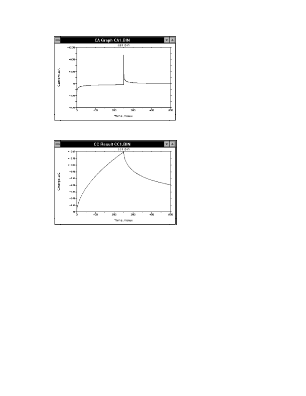
Figure 10-6.

Chronoamperogram (current-time) response for double-potential-step

Figure 10-7.

Chronocoulogram (charge-time) response for double-potential-step

Therefore, both CA and CC can be used to measure one of n, C, A and D using the gradients of these straight line plots, provided the other three constants are known. However, other techniques (e.g., pulse techniques) have lower detection limits, so

and CC are generally not used for concentration measurements. However, A and D are frequently measured using these techniques (1-3).

The relationship between i and t

-1/2

(or Q and t

1/2

) can be used to investigate the

period of time for which the current (or charge) is strictly controlled by diffusion.

-1/2

Figure 10-8 shows a plot of i/t

vs. time. The deviation from ideality at short times is due to the finite length of time required to charge the working electrode to the step potential. The deviations at long times are due to natural convection.

10-15

Page 84

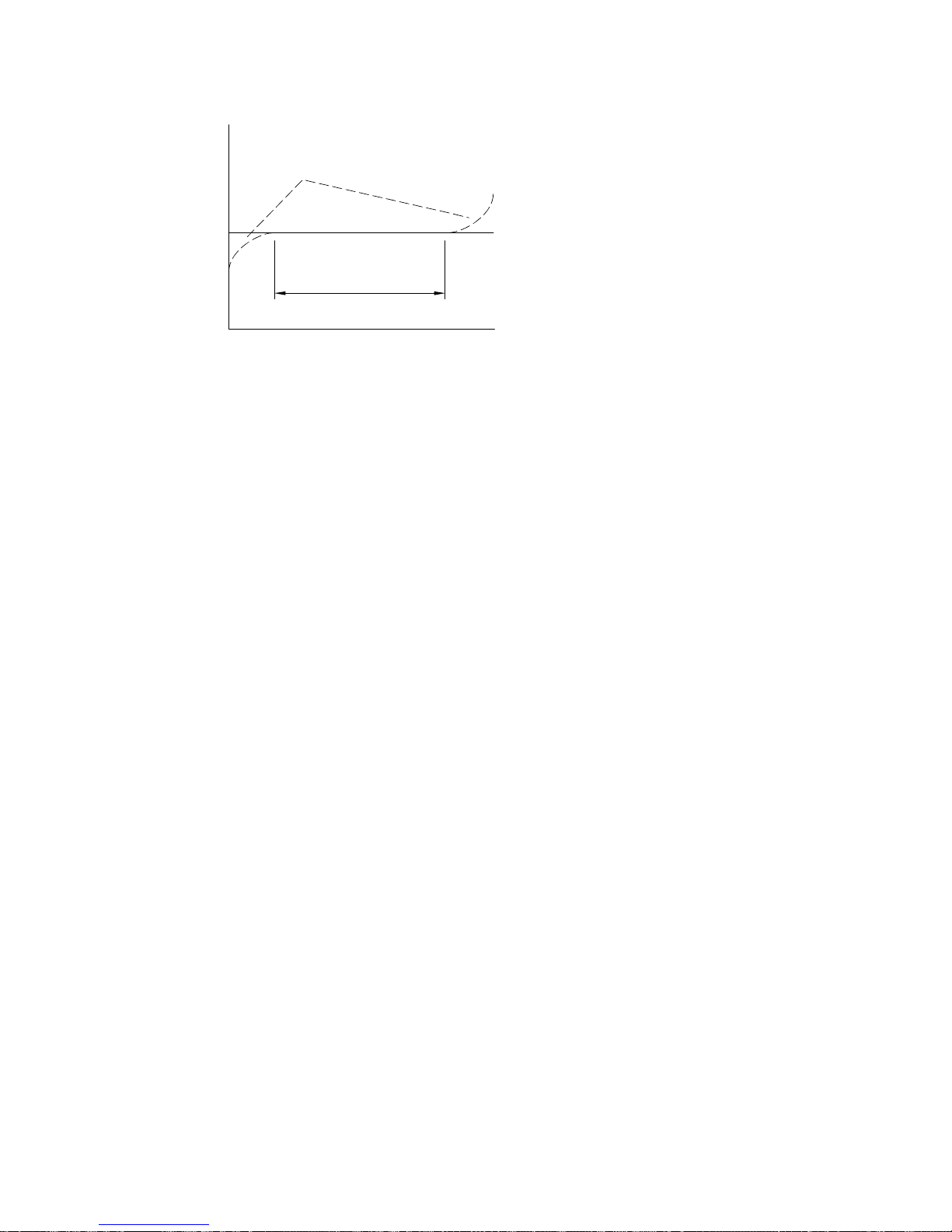
-1/2

i/t

TYPICAL DEVIATIONS

IDEAL

TIME WINDOW

Figure 10-8.

Plot of i/t

-1/2

vs. t for

showing "time window" for condition of planar diffusion.

Although CA and CC are not used to measure absolute concentrations, they can be used to measure changes in concentrations due to homogeneous chemical reactions of the electrolyzed molecules (3,4). This uses the double step technique, and measures the ratio of the forward and backward currents (or charges). If the molecules undergo a chemical reaction after electrolysis in the forward step, then these molecules are not available for electrolysis in the reverse step. Hence, the faster the chemical reaction, the smaller the current/charge on the reverse step. The rate of the chemical reaction can be calculated by measuring the current (or charge) ratio at different pulse widths.

If the final potential is at a value at which the electron transfer does not occur rapidly, then the current (or charge) response may be influenced by the rate of heterogeneous electron transfer as well as the rate of diffusion. The rate of electron transfer can therefore be measured by CA and CC (5).

has several advantages over CA. The signal increases with time, so the latter parts of the response, which are least distorted by the finite charging time of the electrode, offer better signal-to-noise ratios (in addition, any white noise tends to averaged by integration) . In addition, since charge is a summation over the time frame of the experiment, the information from the early response is retained. However, in some instruments, this is not strictly the case, since the charge is obtained by integrating the discrete current values, and some charge is invariably lost. In contrast, in the BAS 100B/W, there is a 'true' charge-to-voltage converter, which means that none of the early information is lost.

Another application of CC which takes advantage of it's ability to retain early information is the detection of species adsorbed to the surface of the working electrode (3). Such species are electrolyzed very rapidly when the potential is stepped. The total charge measured during the CC experiment is

Q = Q

+ Qdl + Q

diff

ads

10-16

Page 85

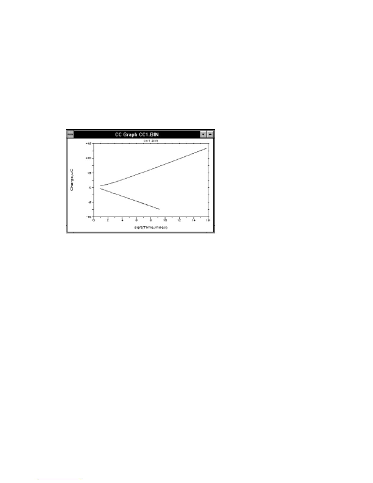
Qdl is the charge due to charging of the working electrode, and Q

is the charge due

ads

to electrolysis of the adsorbed species, and is directly proportional to the surface concentration of the adsorbate. Of the three components, only Q Therefore, the intercept of the Anson plot is Q

+ Q

. One way of calculating Q

ads

is time dependent.

diff

ads

is to measure Qdl by performing the CC experiment on the background solution. However, this assumes that Q

is the same in the presence and absence of the

electroactive species; this is not necessarily true. A more accurate method is to use double step CC, since Q

can be eliminated by calculating the difference between the

intercepts of the forward and reverse Anson plots (Figure 10-9).

Figure 10-9.

Forward and reverse Anson plots.

References

1) BAS Capsule, No. 133 Determination of Electrode Area with

Chronocoulometry

2) BAS Capsule, No. 143 Determination of Diffusion Coefficients Using

Chrono coulometry

3) W.R. Heineman, Curr. Seps 7 (1986) 58-67.

4) BAS Capsule, No. 268 Measurement of Reaction Kinetics Using

Chronocoulometry.

5) A. J. Bard and L. R. Faulkner "Electrochemical Methods" Wiley, New

York, 1980; p. 204-206

STEP

allows a cyclic potential step wave form to be applied to the working electrode. There is no data acquisition in this mode although the response can be monitored at the I

rear panel jack of the BAS 100B. The

OUT

STEP

mode is primarily designed for electrode cleaning and conditioning. The surface of several types of electrodes (e.g., Pt, Au, etc.) have been found to be prepared more reproducibly by applying such a potential wave form to them (the surface is cycled between oxide formation and reduction) In addition, it is often possible to remove adsorbed species with this method.

10-17

Page 86

Mode = CA

General Parameters

Initial E (mV) = 0 -3276 to 3276 High E (mV) = 0 -3276 to 3276 Low E (mV) = 0 -3276 to 3276 Initial Direction = Negative Negative or Positive Pulse width (msec) = 250 1 to 32000 Sensitivity = 1 µA/V 100 mA/V to 100 nA/V (10 pA/V with the

Low Current Module)

Specific parameters

Number of Steps = 2 1 or 2 Quiet Time (sec) = 2 0 to 65535

Graphics Menu

Single Graph

Cottrell plot (

Type

drop-down list box in the

displays the

Current vs. 1/sqrt (Time)

Current vs. Time

) can be selected using the

Graphics Options

plot as the default plot. The

dialog box.

Analysis Menu

The

Auto

option for

Results Graph

displays the plot selected in

Data Type

and the slope, intercept and correlation coefficient are listed in the window. Since data at early time points can be distorted due to the finite time required for the potential step, the

Auto

option uses only the last 80% of the data. An alternative line can be defined by the user through the option (the line is specified by the X values of 2 points on the plot). The units for the slope are mA

Comment:

The maximum data file length is 1000 pts/step.

•

1/2

Mode = CC

General Parameters

Initial E (mV) = 0 -3276 to 3276 Final E (mV) = 0 -3276 to 3276 Pulse Width (msec) = 250 3 to 32000 Sensitivity = 1 µC/V 100 nC/V to 10 µC/V

Data

Main

Manual

Specific Parameters

Number of Steps = 2 1 or 2 Quiet Time (sec) = 2 0 to 65535

10-18

Page 87

Comments

The maximum data file length is 1000 points/step. The circuitry for CC is a direct charge-to-voltage converter. The integrating capacitor that is used to accumulate the charge in the 10 µC/V

Sensitivity

range is automatically discharged and reset to zero when it nears the voltage saturation level. This operation allows a much greater charge to be measured during the experiment. Discharging the capacitor requires 0.5 msec during which time no charge is measured. We have never had a situation where thishas caused a noticeable error in the output, since discharge typically occursafter the initial large current transients have decayed and the current isrelatively small (so the charge lost over 0.5 msec is less than the resolution of the instrument and the expected precision of the experiment). However, errors can occur if the initial current are very large, since this may cause discharging at short times. Such errors are shown by discontinuities in the

Charge vs. Time

plot. If this occurs, the initial current must be decreased by, for

example, decreasing the concentration and/or the electrode surface area.

The automatic discharge is not allowed for the 100 nC/V and 1 µC/V ranges, since the charge lost during the 0.5 msec may be significant.

Too much current may also cause the digital accumulators to overload. This occurs after 32 discharge-charge cycles, and is shown by sharp discontinuities in

Charge vs. Time

the

plot as the charge drops to zero.

Graphics Menu

Single Graph

Anson plot (

displays the

Charge vs. sqrt (Time)

drop-down list box in the

Charge vs. Time

)can be selected using the

Graph Options

plot as the default plot. The

Data Type

dialog box.

Analysis Menu

The

Auto

option for

Results Graph

displays the plot selected in

Data Type

and the slope, intercept and correlation coefficient are listed in the window. Since data at early time points can be distorted due to the finite time required for the potential step, the

Auto

option uses only the last 80% of the data. An alternative line can be defined by the user through the Manual option (the line is specified by the X values of 2 points on the plot). The slope is reported in units of c/ms

1/2

Main

10-19

Page 88

Mode = STEP

General Parameters

Initial E (mV) = 0 -3276 to 3276 High E (mV) = 0 -3276 to 3276 Low E (mV) = 0 -3276 to 3276 Initial Direction = Negative Negative or Positive Pulse width (msec) = 250 1 to 32000 Number of Cycles = 1 0 to 65535 Sensitivity = 1 µA/V 100 mA/V to 10 pA/V

Specific parameters

Quiet Time (sec) = 2 0 to 65535

Comments

When the

Number of Cycles

until it is stopped by the user.

is set to 0, the cycling continues indefinitely

10-20

Page 89

10.3 Pulse Techniques (SCP, NPV/P, DPV/P)

The basis of all pulse techniques is the difference in the rate of decay of background and faradaic currents following a potential step. The background current decays exponentially, whereas the faradaic current decays as a function of 1/(time) the rate of decay of the background current is considerably faster than the decay of the faradaic current. The background current is negligible at a time of 5R

the potential step (R ranges from µs to ms). Therefore, after this time, the measured current consists solely

of the faradaic current; that is, measuring the current at the end of the potential pulse allows discrimination between the faradaic and charging current.

The important parameters for Pulse techniques are as follow:

Pulse Amplitude

Pulse Width

Sample Width

current is measured. It must be at least 2 msec shorter than the current is sampled and averaged 16 times per msec. The default the time required for 1 line cycle.

is the duration of the potential pulse in msec.

is the time (in msec) at the end of the pulse during which the

is the time constant for a given electrochemical cell, and

uCdl

is the height of the potential pulse in mV.

Pulse Width

Sample Width

1/2

uCdl

; that is,

after

. The

Pulse Period/Dropping Time

(in msec) and must be at least twice the voltammetry experiments, whereas experiments, in which the potential pulse, current sampling and renewal of the mercury drop are coordinated (this is controlled by the BAS 100B/W). As discussed above, the current is sampled at the end of the pulse, and the mercury drop is knocked off at the end of the end of the pulse). For polarography experiments using a dropping mercury electrode (DME), the advantage of sampling the current at the end of the drop lifetime is that the rate of change of the surface area (which contributes to the charging current) is at a minimum at this point.

Three different pulse techniques are available on the BAS 100B/W Electrochemical Workstation. These differ in the potential pulse waveforms and the number of sampling times. The discrimination against the charging current that is inherent in these techniques leads to lower detection limits (compared to linear sweep techniques), which make these techniques suitable for quantitative analysis.

- This is the time required for one potential cycle

Pulse Width. Pulse Period

Dropping Time

Sample Width

10-21

applies to polarography

(which coincides with the

is used for

Page 90

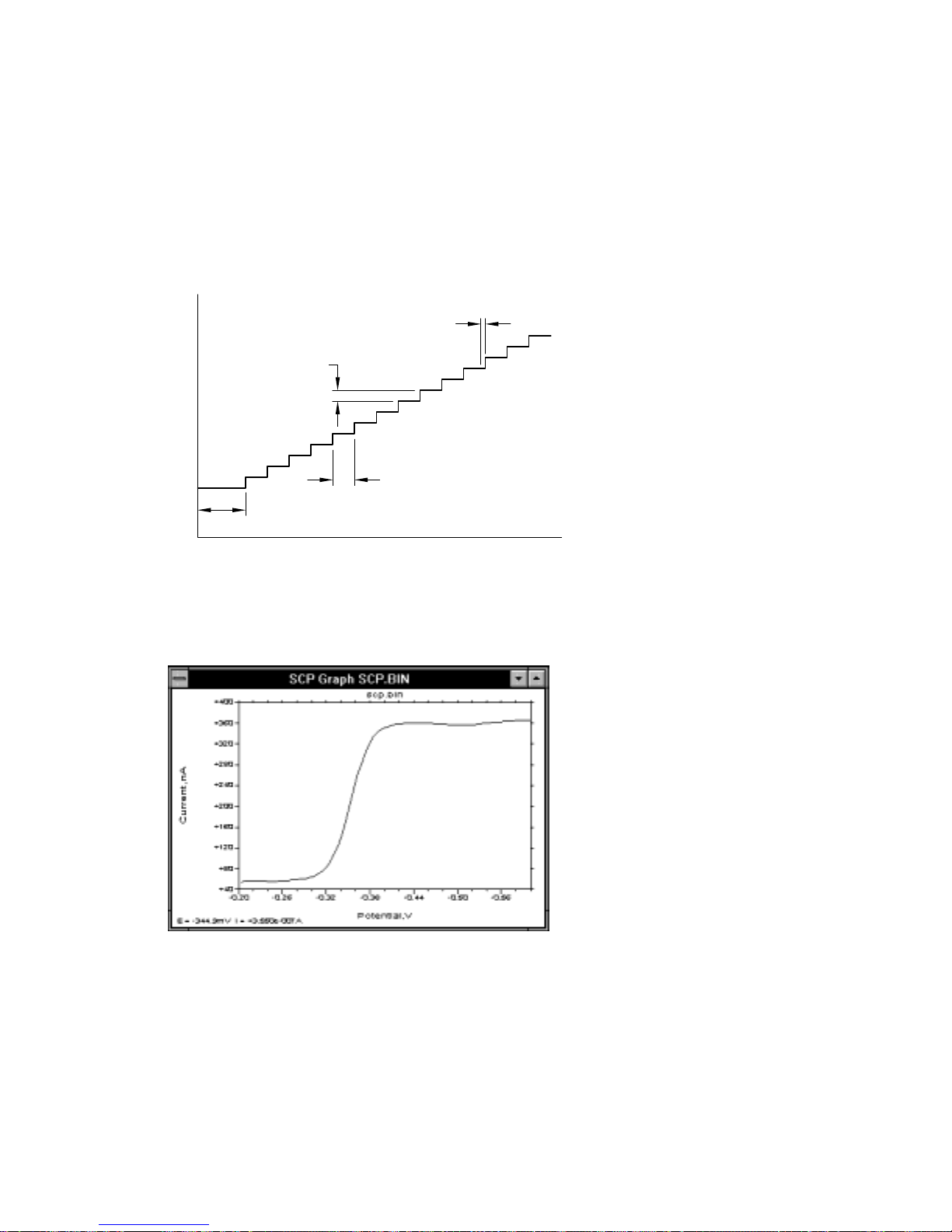
Sampled Current Polarography (

SCP

) or Tast polarography is a modification of the classical D.C. polarography experiment, and was designed to reduce the effect the changing surface area of the mercury drop. The potential wave form is shown in Figure 10-10. The potential is varied in a series of steps (it is held at each step for the

Drop Time

), and the current is sampled at the end of each drop. The

the size of the potential step can be varied (through variation of the

Drop Time

Scan Rate

and

). This

potential waveform is often referred as a staircase waveform.

-E SAMPLING WIDTH

STEP

DROP TIME

QUIET TIME

Figure 10-10.

Potential wave form for

SCP

The current response is shown in Figure 10-11. The limiting current (id) is given by the Ilkovic equation:

Figure 10-11.

id = 708nD

1/2Cm2/3τ1/6

Typical current response for

SCP

where: n = number of electrons transferred/molecule

D = diffusion coefficient (cm m = mercury flow rate (mg/s)

= sampling interval (s)

/s)

10-22

Page 91

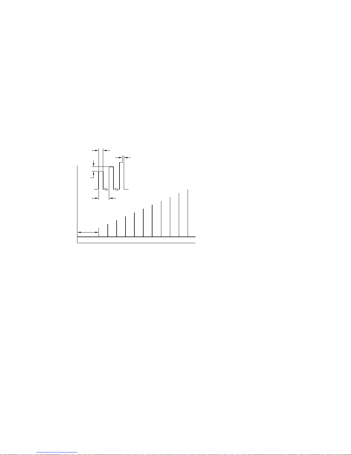
The sensitivity and detection limit of

A/mM and 10

-5

M). The major advantage of

SCP

are similar to those of DC polarography (5

SCP

over D.C. polarography is the smoothed current output, which facilitates measurement of the half-wave potentials and limiting currents.

Although this is a essentially a polarographic technique, it can be used as a slow scan rate voltammetry technique. This modification is often called "staircase" voltammetry.

The potential wave form for Normal Pulse Voltammetry/Polarography

(NPV/P)

is shown in Figure 10-12, and consists of a series of pulses of increasing amplitude, with the potential returning to the initial value in between the pulses.

PULSE WIDTH

SAMPLE

∆

QUIET

TIME

Figure 10-12.

Potential wave form for

Consider a reduction. If

WIDTH

PULSE PERIOD

Initial E

NPV/P

is well positive of the redox potential, the application of small amplitude pulses does not cause any faradaic reaction, so there is no faradaic current response. When the pulse amplitude is sufficiently large that the pulsed potential is around the redox potential, there is a faradaic reaction in response to the pulse (assuming moderately rapid electron transfer kinetics), and the magnitude of this faradaic current may depend on both the rate of diffusion and the rate of electron transfer. When the pulsed potentials are sufficiently negative of the redox potential that the electron transfer occurs rapidly, the faradaic current depends only of the rate of diffusion; that is, a limiting current has been reached. This current response is shown in Figure 10-13. The sigmoidal shape is similar to the shape of the curve obtained in the classical polarography experiment, which gives rise to the name of normal for this pulse technique. The limiting current for

SCP

for detection limit (10

, and is therefore a more sensitive technique (30 µA/mM) and has a lower

-6

M).

NPV/P

is greater than that

There is a variation of this technique called Reverse Pulse Voltammetry/Polarography (RPV/P). In

NPV/P

occurs, whereas in RPV/P, the initial potential is at a value at which the faradaic

, the initial potential is at a value at which no faradaic reaction

10-23

Page 92

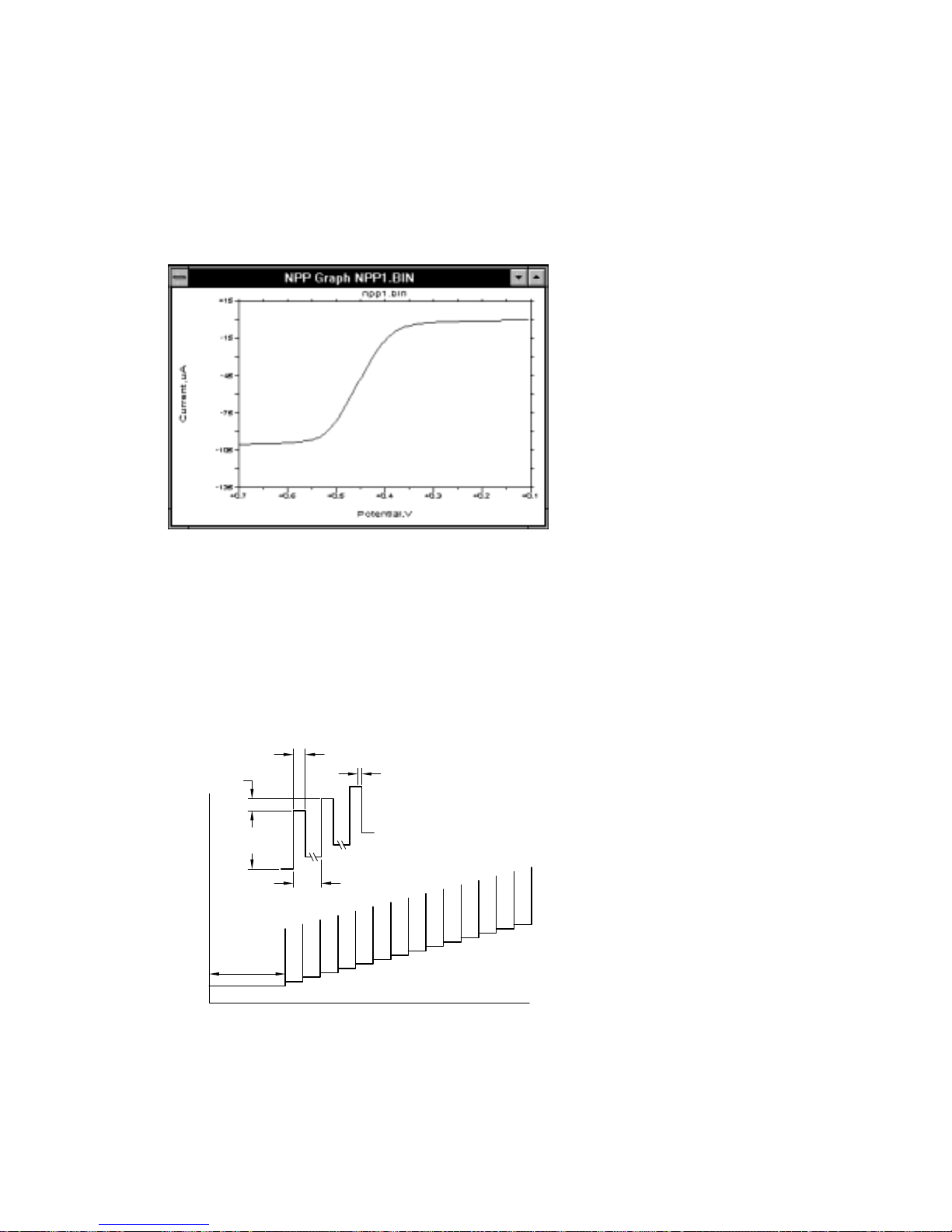
reaction of interest occurs at the diffusion limited rate. This technique is useful for discriminating between a reversible redox process (rapid electron transfer) and an irreversible redox process (slow electron transfer on the reverse step), since both can be detected by NPV/P, whereas only the reversible process can be detected by RPV/P. One example of this is the detection of metal ions (reversible) in the presence of oxygen (irreversible).

Figure 10-13.

Typical current response for

Differential Pulse Voltammetry/Polarography ( two techniques in that the current is sampled twice in each potential wave form is shown in Figure 10-14. The

NPV/P

DPV/P

) is different from the previous

Pulse Amplitude

Pulse Period

is constant with

. The

respect to the base potential, and the base potential increases in small steps; that is, the potential wave form consists of small amplitude pulses superimposed upon a staircase waveform.

PULSE WIDTH

∆

PULSE

AMPLITUDE

QUIET

TIME

SAMPLE WIDTH

PULSE PERIOD

Figure 10-14.

Potential wave form for

The current is sampled just before the pulse (i1) and at the end of the pulse (i2), and the difference (i

- i1) is recorded as a function of the base potential. Consider a

DPV/P

10-24

Page 93

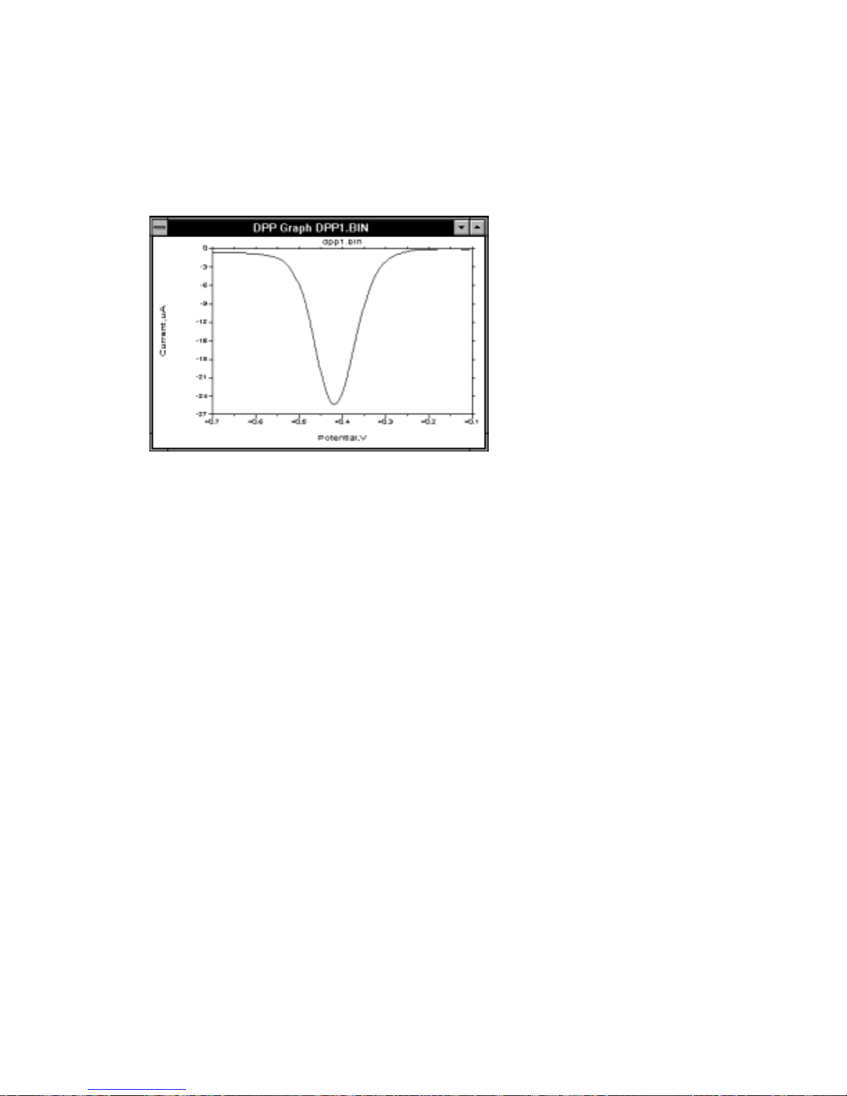
reduction. At potentials well positive of the redox potential, there is no faradaic reaction is response to the pulse, so the differential current is zero. At potentials around the redox potential, the differential current reaches a maximum and decreases to zero as the current becomes diffusion-controlled. The current response is therefore a symmetric peak (Figure 10-15).

Figure 10-15.

The sensitivity of

Typical current response for

DPV/P

the detection limit of

is intermediate between

DPV/P

is significantly lower (10

DPV/P

discrimination against the charging current.

Mode = SCP General Parameters

Initial E (mV) = 0 -3276 to 3276 Final E (mV) = 0 -3276 to 3276 Sensitivity = 1µA/V 100 mA/V to 100 nA/V (10 pA/V with the

Low Current Module)

Specific Parameters

Scan Rate (mV/s) = 4 1 to 200 Sample Width (msec) = 17 1 to 250 Drop Time (msec) = 1000 100 to 8000 Quiet Time (sec) = 2 0 to 65535

Comments

NPV/P

SCP

and

-7

M) due to more effective

(20 µA/mM), but

a) Increasing the

b) The step height (or sampling interval) is the product of the

Dropping Time

Sample Width

can reduce noise.

(e.g. the default values is 4 mV).

10-25

Scan Rate

and the

Page 94

Graphics Menu

Single Graph

displays the current vs. potential plot.

Analysis Menu

The

Auto

option for

Results Graph

displays the current vs. potential plot, and the half-wave potential and limiting current are listed in the window. Alternative baselines can be set by the user through the option.

Mode = NPV/P General Parameters

Initial E (mV) = 0 -3276 to 3276 Final E (mV) = 0 -3276 to 3276 Sensitivity = 1µA/V 100 mA/V to 100 nA/V (10 pA/V with the

Low Current Module)

Specific Parameters

Scan Rate (mV/sec) = 20 (4) 1 to 200 Sample Width (msec) = 17 1 to 250 Pulse Width (msec) = 50 3 to 2000 Pulse Period (msec) = 200 40 to 8000 Drop Time (msec) = 1000 100 to 8000 Quiet Time (sec) = 2 (0) 0 to 65535

Main

Manual

Comments

a) The

Pulse Period

parameter value for

is used in

NPP

NPV

, the

Drop Time

is different from that for

parentheses

b) Increasing the

Sample Width

can reduce the response noise.

c) The sample interval is equal to the product of the

Period

Drop Time

(or

) (e.g., the default value is 4 mV).

Graphics Menu

Single Graph

displays the current vs. potential plot.

NPP

. When thedefault

NPV

Scan Rate

, it is shown in

and the

Pulse

10-26

Page 95

Analysis Menu

The

Auto

option for

Results Graph

displays the current vs. potential plot, and the half-wave potential and limiting current are listed in the window. Alternative baselines can be set by the user through the option.

Mode = DPV/P

General Parameters

Initial E (mV) = 0 -3276 to 3276 Final E (mV) = 0 -3276 to 3276 Sensitivity = 1µA/V 100 mA/V to 100 nA/V (10 pA/V with the

Low Current Module)

Specific Parameters

Scan Rate (mV/sec) = 20 (4) 1 to 200 Pulse Amplitude (mV) = 50 -250 to 250 Sample Width (msec) = 17 1 to 250 Pulse Width (msec) = 50 3 to 2000 Pulse Period (msec) = 200 40 to 8000 Drop Time (msec) = 1000 100 to 8000 Quiet Time (sec) = 2 (0) 0 to 65535

Main

Manual

Comments

Pulse Period

is used for

default parameter value for

DPV

DPP

Drop Time

, and

is used for

is different from that for

parentheses.

b) The product of the

than the

c) When the

Pulse Amplitude

Pulse Period

, and greater than 1 mV.

is negative, the direction of the

Drop Time

(or

) and

to that of the scan.

d) Increasing the

Sample Width

can reduce the noise.

e) The sample interval is equal to the product of the

Period

Drop Time)

(or

(e.g., the default value is 4 mV).

Graphics Menu

Single Graph

displays the current vs. potential plot.

DPV

Scan Rate

Pulse

Scan Rate

DPP

. When the

, it is shown in

must be less

is opposite

and the

Pulse

10-27

Page 96

Analysis Menu

The

Auto

option for

Results Graph

displays the current vs. potential plot, and the peak potential and peak current are listed in the Alternative baselines can be set by the user through the

Manual

Main

option.

window.

10-28

Page 97

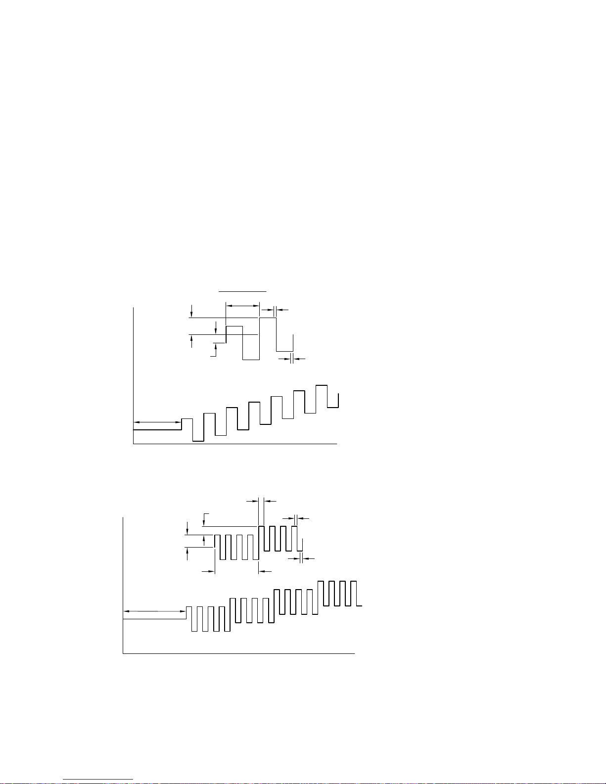
10.4 Square Wave Techniques (OSWV, BSWV/P)

Square wave techniques are related to both pulse techniques and A.C. voltammetric techniques. They are similar to peak and that there is effective discrimination against background charging currents. The chief advantages are the greater sensitivity and the faster speed (for

There are two different square wave potential wave forms available on the BAS 100B/W, Osteryoung (

OSWV

10-16 and Figure 10-17.

FREQUENCY

S.W. AMPLITUDE

DPV/P

) and Barker (

in that the current response is a symmetric

OSWV

BSWV/P

SAMPLE WIDTH (i )

). These are shown in Figure

QUIET

TIME

Figure 10-16.

PULSE

AMPLITUDE

QUIET TIME

STEP

Potential wave form for

PULSE WIDTH

∆

DROPPING TIME

OSWV

SAMPLE WIDTH (i )

Figure 10-17.

Potential wave form for

BSWV/P

10-29

Page 98

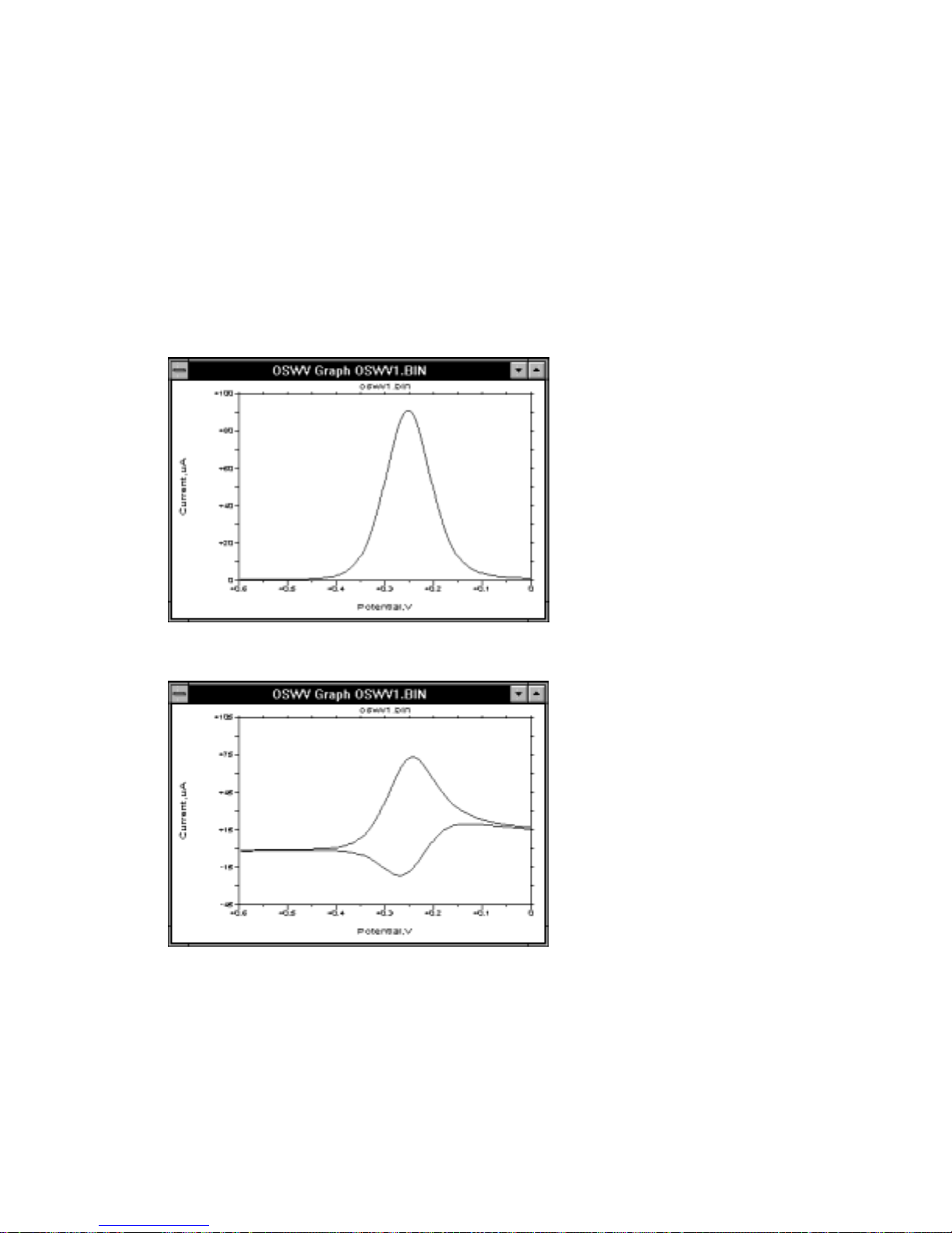
The potential wave form for

OSWV

consists of a square wave superimposed on a staircase wave form. It can also be viewed as a series of pulses alternating in direction (hence, the relation to both pulse and A.C. techniques). The current is sampled at the end of each of the pulses (or half-cycles). The default current output is the difference current (Figure 10-18), but the forward current (i

) can also be examined (Figure 10-19). For a reversible system, the reverse current

) and reverse current

is significant, so the difference current is greater than either the forward or reverse currents. This is one reason for the greater sensitivity of

DPV/P

. The magnitude of the reverse current can also be used to investigate the

OSWV

compared with

reversibility of the electron transfer.

Figure 10-18.

Figure 10-19.

Difference current response for

Forward and reverse current responses for

The waveform for

BSWV/P

is similar to that for

OSWV and BSWV/P

OSWV

. The main difference is that the samples are collected and averaged over a number of cycles. In addition, only the difference current is available (Figure 10-18). Due to the signal averaging, is significantly slower than

OSWV

BSWV/P

10-30

Page 99

The other advantage of

OSWV

compared to

DPV/P

is its speed. Scan rates of up to 80 V/s are available on the BAS 100B/W, although scan rates of 100s mV/s to a few V/s are typically used (note that the scan rate for frequency). This is significantly faster than the scan rate for mV/s). In addition, the sensitivity of

OSWV

depends on the square wave

(compared with

DPV/P

DPP/V

(ca. 10 -20

) increases with increasing scan rate, even for irreversible processes. The greater sensitivity and faster speed of

OSWV

has increased the popularity of this technique for quantitative determination of electroactive species in solution. The detection limit can be further lowered by using stripping methods, which are discussed in section 10.6.

Mode = OSWV

General Parameters

Initial E (mV) = 0 -3276 to 3276 Final E (mV) = 0 -3276 to 3276 Sensitivity = 1µA/V 100 mA/V to 100 nA/V (10 pA/V with the

Low Current Module)

Specific Parameters

Step E (mV) = 4 1 to 40 S.W. Amplitude (mV) = 25 1 to 250 S.W. Frequency (Hz) = 15 1 to 2000 Sampling Points = 256 1, 16, 256 Quiet Time (sec) = 2 0 to 65535

Comments

a) The

S.W. Amplitude

must be greater than

Step E

(which is the potential step

height for the staircase potential wave form).

Sampling Points

is the number of current samples taken and averaged at the

end of each half-cycle. The 3 current sampling options are:

i) 256 samples taken and averaged over 1 line cycle (maximum

Frequency

ii) 16 samples taken and averaged over 1 msec (maximum

= 15 Hz).

S.W. Frequency

= 250 Hz)

iii) 1 sample taken (maximum

S.W. Frequency

= 2000 Hz).

The maximum frequency for each option is such that the sampling time is no longer than 1/2 of each half-cycle. The option is selected by the software.

c) The scan rate (mV/s) is the product of the

d) The sample interval is equal to

Step E

S.W. Frequency

and

Step E

e) Maximum data file length is 1279 points.

S.W.

10-31

Page 100

Graphics Menu

Single Graph

specified in the

displays the current vs. potential plot(s) of the

Graph

Results Options

and

dialog boxes.

Data Sets

Analysis Menu

Auto

The of the

option for

Data Sets

and the peak potential and peak current are listed in the Alternative baselines can be set by the user through the

Results Graph

specified in the

displays the current vs. potential plot(s)

Graph

Results Options

and

Main

Manual

dialog boxes,

window.

option.

Mode = BSWV/P

General Parameters

Initial E (mV) = 0 -3276 to 3276 Final E (mV) = 0 -3276 to 3276 Sensitivity = 1µA/V 100 mA/V to 100 nA/V (10 pA/V with the

Low Current Module)

Specific Parameters

Scan Rate (mV/s) = 4 1 to 200 S.W. Amplitude (mV) = 25 1 to 250 S.W. Frequency (Hz) = 14 5 to 250 Drop Time (msec) = 1500 1500 to 8000 Quiet time (sec) = 2 (0) 0 to 65535

Comments

a) Parameters values in parentheses refer to

used for

BSWP

(the analogous parameter for

BSWP

BSWV

. The

Drop Time

Step Period

, the

at 1500 msec).

b) The number of current samples averaged during each

Period

) is determined by the

S.W. Frequency

Drop Time

c) Sampling width is fixed at 1/4 cycle time period for all frequencies.

d) The sample interval is the product of the

Step Period

) (e.g., the default value is 6 mV).

Scan Rate

and the

Drop Time

Graphics Menu

Single Graph

and reverse current plots are not available for

displays the difference current vs. potential plot. The forward

BSWV/P

10-32

is only

, is set

(or

Step

(or