Autodesk Inventor Inventor Simulation - 2009 Getting Started

Autodesk Inventor Simulation 2009

Getting Started

January 2008Part No. 462A1-050000-PM02A

©

2008 Autodesk, Inc. All Rights Reserved. Except as otherwise permitted by Autodesk, Inc., this publication, or parts thereof, may not be

reproduced in any form, by any method, for any purpose.

Certain materials included in this publication are reprinted with the permission of the copyright holder.

Trademarks

The following are registered trademarks or trademarks of Autodesk, Inc., in the USA and other countries: 3DEC (design/logo), 3December,
3December.com, 3ds Max, ActiveShapes, Actrix, ADI, Alias, Alias (swirl design/logo), AliasStudio, Alias|Wavefront (design/logo), ATC, AUGI,
AutoCAD, AutoCAD Learning Assistance, AutoCAD LT, AutoCAD Simulator, AutoCAD SQL Extension, AutoCAD SQL Interface, Autodesk, Autodesk
Envision, Autodesk Insight, Autodesk Intent, Autodesk Inventor, Autodesk Map, Autodesk MapGuide, Autodesk Streamline, AutoLISP, AutoSnap,
AutoSketch, AutoTrack, Backdraft, Built with ObjectARX (logo), Burn, Buzzsaw, CAiCE, Can You Imagine, Character Studio, Cinestream, Civil
3D, Cleaner, Cleaner Central, ClearScale, Colour Warper, Combustion, Communication Specification, Constructware, Content Explorer,
Create>what's>Next> (design/logo), Dancing Baby (image), DesignCenter, Design Doctor, Designer's Toolkit, DesignKids, DesignProf, DesignServer,
DesignStudio, Design|Studio (design/logo), Design Your World, Design Your World (design/logo), DWF, DWG, DWG (logo), DWG TrueConvert,
DWG TrueView, DXF, EditDV, Education by Design, Exposure, Extending the Design Team, FBX, Filmbox, FMDesktop, Freewheel, GDX Driver,
Gmax, Heads-up Design, Heidi, HOOPS, HumanIK, i-drop, iMOUT, Incinerator, IntroDV, Inventor, Inventor LT, Kaydara, Kaydara (design/logo),
LocationLogic, Lustre, Maya, Mechanical Desktop, MotionBuilder, Mudbox, NavisWorks, ObjectARX, ObjectDBX, Open Reality, Opticore,
Opticore Opus, PolarSnap, PortfolioWall, Powered with Autodesk Technology, Productstream, ProjectPoint, ProMaterials, Reactor, RealDWG,
Real-time Roto, Recognize, Render Queue, Reveal, Revit, Showcase, ShowMotion, SketchBook, SteeringWheels, StudioTools, Topobase, Toxik,
ViewCube, Visual, Visual Bridge, Visual Construction, Visual Drainage, Visual Hydro, Visual Landscape, Visual Roads, Visual Survey, Visual Syllabus,
Visual Toolbox, Visual Tugboat, Visual LISP, Voice Reality, Volo, Wiretap, and WiretapCentral

The following are registered trademarks or trademarks of Autodesk Canada Co. in the USA and/or Canada and other countries: Backburner,
Discreet, Fire, Flame, Flint, Frost, Inferno, Multi-Master Editing, River, Smoke, Sparks, Stone, and Wire

All other brand names, product names or trademarks belong to their respective holders.

Disclaimer

THIS PUBLICATION AND THE INFORMATION CONTAINED HEREIN IS MADE AVAILABLE BY AUTODESK, INC. "AS IS." AUTODESK, INC. DISCLAIMS
ALL WARRANTIES, EITHER EXPRESS OR IMPLIED, INCLUDING BUT NOT LIMITED TO ANY IMPLIED WARRANTIES OF MERCHANTABILITY OR
FITNESS FOR A PARTICULAR PURPOSE REGARDING THESE MATERIALS.

Published by:
Autodesk, Inc.
111 Mclnnis Parkway
San Rafael, CA 94903, USA

Contents

Stress Analysis . . . . . . . . . . . . . . . . . . . . . . . . . . . 1

Chapter 1 Get Started With Stress Analysis . . . . . . . . . . . . . . . . . . 3

About Autodesk Inventor Simulation . . . . . . . . . . . . . . . . . . . 3

Learning Autodesk Inventor Simulation . . . . . . . . . . . . . . . . . . 3

Using Help . . . . . . . . . . . . . . . . . . . . . . . . . . . . . . . . . 4

Using Stress Analysis Tools . . . . . . . . . . . . . . . . . . . . . . . . . 5

Understanding the Value of Stress Analysis . . . . . . . . . . . . . . . . 6

Understanding How Stress Analysis Works . . . . . . . . . . . . . . . . 7

Analysis Assumptions . . . . . . . . . . . . . . . . . . . . . . . . 7

Interpreting Results of Stress Analysis . . . . . . . . . . . . . . . . . . . 9

Equivalent Stress . . . . . . . . . . . . . . . . . . . . . . . . . . 10

Maximum and Minimum Principal Stresses . . . . . . . . . . . . 10

Deformation . . . . . . . . . . . . . . . . . . . . . . . . . . . . . 10

Safety Factor . . . . . . . . . . . . . . . . . . . . . . . . . . . . . 10

Frequency Modes . . . . . . . . . . . . . . . . . . . . . . . . . . 11

Chapter 2 Analyze Models . . . . . . . . . . . . . . . . . . . . . . . . . . 13

Working in the Stress Analysis Environment . . . . . . . . . . . . . . . 13

Running Stress Analysis . . . . . . . . . . . . . . . . . . . . . . . . . . 14

Verifying Material . . . . . . . . . . . . . . . . . . . . . . . . . . 15

Applying Loads . . . . . . . . . . . . . . . . . . . . . . . . . . . 16

Applying Constraints . . . . . . . . . . . . . . . . . . . . . . . . 19

iii

Setting Parameters . . . . . . . . . . . . . . . . . . . . . . . . . . 20

Feature Suppression Tracking . . . . . . . . . . . . . . . . . . . . 21

Setting Solution Options . . . . . . . . . . . . . . . . . . . . . . 21

Obtaining Solutions . . . . . . . . . . . . . . . . . . . . . . . . . 23

Running Modal Analysis . . . . . . . . . . . . . . . . . . . . . . . . . 23

Chapter 3 View Results . . . . . . . . . . . . . . . . . . . . . . . . . . . . 25

Using Results Visualization . . . . . . . . . . . . . . . . . . . . . . . . 25

Editing the Color Bar . . . . . . . . . . . . . . . . . . . . . . . . . . . 26

Reading Stress Analysis Results . . . . . . . . . . . . . . . . . . . . . . 28

Interpreting Results Contours . . . . . . . . . . . . . . . . . . . . 28

Animate Results . . . . . . . . . . . . . . . . . . . . . . . . . . . 29

Setting Results Display Options . . . . . . . . . . . . . . . . . . . 30

Chapter 4 Revise Models and Stress Analyses . . . . . . . . . . . . . . . . 31

Changing Model Geometry . . . . . . . . . . . . . . . . . . . . . . . . 31

Changing Solution Conditions . . . . . . . . . . . . . . . . . . . . . . 32

Updating Results of Stress Analysis . . . . . . . . . . . . . . . . . . . . 34

Chapter 5 Generate Reports . . . . . . . . . . . . . . . . . . . . . . . . . 35

Running Reports . . . . . . . . . . . . . . . . . . . . . . . . . . . . . . 35

Interpreting Reports . . . . . . . . . . . . . . . . . . . . . . . . . . . . 35

Summary . . . . . . . . . . . . . . . . . . . . . . . . . . . . . . 36

Introduction . . . . . . . . . . . . . . . . . . . . . . . . . . . . . 36

Scenario . . . . . . . . . . . . . . . . . . . . . . . . . . . . . . . 36

Appendices . . . . . . . . . . . . . . . . . . . . . . . . . . . . . 37

Saving and Distributing Reports . . . . . . . . . . . . . . . . . . . . . 37

Saving Reports . . . . . . . . . . . . . . . . . . . . . . . . . . . . 37

Printing Reports . . . . . . . . . . . . . . . . . . . . . . . . . . . 37

Distributing Reports . . . . . . . . . . . . . . . . . . . . . . . . . 38

Chapter 6 Manage Stress Analysis Files . . . . . . . . . . . . . . . . . . . 39

Creating and Using Analysis Files . . . . . . . . . . . . . . . . . . . . . 39

Understanding File Relationships . . . . . . . . . . . . . . . . . . 40

Repairing Disassociated Files . . . . . . . . . . . . . . . . . . . . . . . 40

Copying Geometry Files . . . . . . . . . . . . . . . . . . . . . . 41

Resolving File Link Failures . . . . . . . . . . . . . . . . . . . . . 41

Creating New Analysis Files . . . . . . . . . . . . . . . . . . . . . 42

Exporting Analysis Files . . . . . . . . . . . . . . . . . . . . . . . . . . 42

Simulation . . . . . . . . . . . . . . . . . . . . . . . . . . . . . 43

iv | Contents

Chapter 7 Get Started with Simulation . . . . . . . . . . . . . . . . . . . 45

About Autodesk Inventor Simulation . . . . . . . . . . . . . . . . . . . 45

Learning Autodesk Inventor Simulation . . . . . . . . . . . . . . . . . 46

Using Help . . . . . . . . . . . . . . . . . . . . . . . . . . . . . . . . . 46

Understanding Simulation Tools . . . . . . . . . . . . . . . . . . . . . 47

Simulation Assumptions . . . . . . . . . . . . . . . . . . . . . . . . . 47

Interpreting Simulation Results . . . . . . . . . . . . . . . . . . . . . 47

Relative Parameters . . . . . . . . . . . . . . . . . . . . . . . . . 47

Coherent Masses and Inertia . . . . . . . . . . . . . . . . . . . . 48

Continuity of Laws . . . . . . . . . . . . . . . . . . . . . . . . . 48

Chapter 8 Simulate Motion . . . . . . . . . . . . . . . . . . . . . . . . . . 49

Understanding Degrees of Freedom . . . . . . . . . . . . . . . . . . . . 49

Understanding Constraints . . . . . . . . . . . . . . . . . . . . . . . . 49

Converting Assembly Constraints . . . . . . . . . . . . . . . . . . . . 50

Defining Forces . . . . . . . . . . . . . . . . . . . . . . . . . . . . . . 54

Creating Simulations . . . . . . . . . . . . . . . . . . . . . . . . . . . 56

Chapter 9 Construct Moving Assemblies . . . . . . . . . . . . . . . . . . 59

Creating Rigid Bodies . . . . . . . . . . . . . . . . . . . . . . . . . . . 59

Adding Joints . . . . . . . . . . . . . . . . . . . . . . . . . . . . . . . 60

Working with Z Axes . . . . . . . . . . . . . . . . . . . . . . . . . . . 61

Working with Joint Triad . . . . . . . . . . . . . . . . . . . . . . . . . 62

Chapter 10 Simulation Tools . . . . . . . . . . . . . . . . . . . . . . . . . . 73

Input Grapher . . . . . . . . . . . . . . . . . . . . . . . . . . . . . . . 73

Output Grapher . . . . . . . . . . . . . . . . . . . . . . . . . . . . . . 76

Index . . . . . . . . . . . . . . . . . . . . . . . . . . . . . . . . 79

Contents | v

vi

Stress Analysis

Part 1 of this manual presents the getting started information for Stress Analysis in the
Autodesk® Inventor™ Simulation software. This add-on to the Autodesk Inventor part and
sheet metal environments provides the capability to analyze the stress and frequency responses
of mechanical part designs.

1

2

Get Started With Stress Analysis

Autodesk® Inventor™ Simulation software provides a combination of industry-specific tools
that extend the capabilities of Autodesk Inventor for completing complex machinery and
other product designs.

Stress Analysis in Autodesk Inventor Simulation is an add-on to the Autodesk Inventor part
and sheet metal environments. It provides the capability to analyze the stress and frequency
responses of mechanical part designs.

This chapter provides basic information about the stress analysis environment and the
workflow processes necessary to analyze loads and constraints placed on a part.

1

About Autodesk Inventor Simulation

Built on the Autodesk Inventor application, Autodesk Inventor Simulation
includes several different modules. The first module included in this manual is
Stress Analysis. It provides functionality for stressing and analyzing mechanical
product designs.

This manual provides basic conceptual information to help get you started and
specific examples that introduce you to the capabilities of Stress Analysis in
Autodesk Inventor Simulation.

Learning Autodesk Inventor Simulation

We assume that you have a working knowledge of the Autodesk Inventor
Simulation interface and tools. If you do not, use Help for access to online

3

documentation and tutorials, and complete the exercises in the Autodesk
Inventor Simulation Getting Started manual.

At a minimum, we recommend that you understand how to:

■ Use the assembly, part modeling, and sketch environments and browsers.

■ Edit a component in place.

■ Create, constrain, and manipulate work points and work features.

■ Set color styles.

Be more productive with Autodesk® software. Get trained at an Autodesk
Authorized Training Center (ATC®) with hands-on, instructor-led classes to
help you get the most from your Autodesk products. Enhance your productivity

with proven training from over 1,400 ATC sites in more than 75 countries.
For more information about training centers, contact [e-mail]
or visit the online ATC locator at www.autodesk.com/atc.

We also recommend that you have a working knowledge of Microsoft
Windows NT® 4.0, Windows® 2000, or Windows® XP, and a working
knowledge of concepts for stressing and analyzing mechanical assembly

designs.

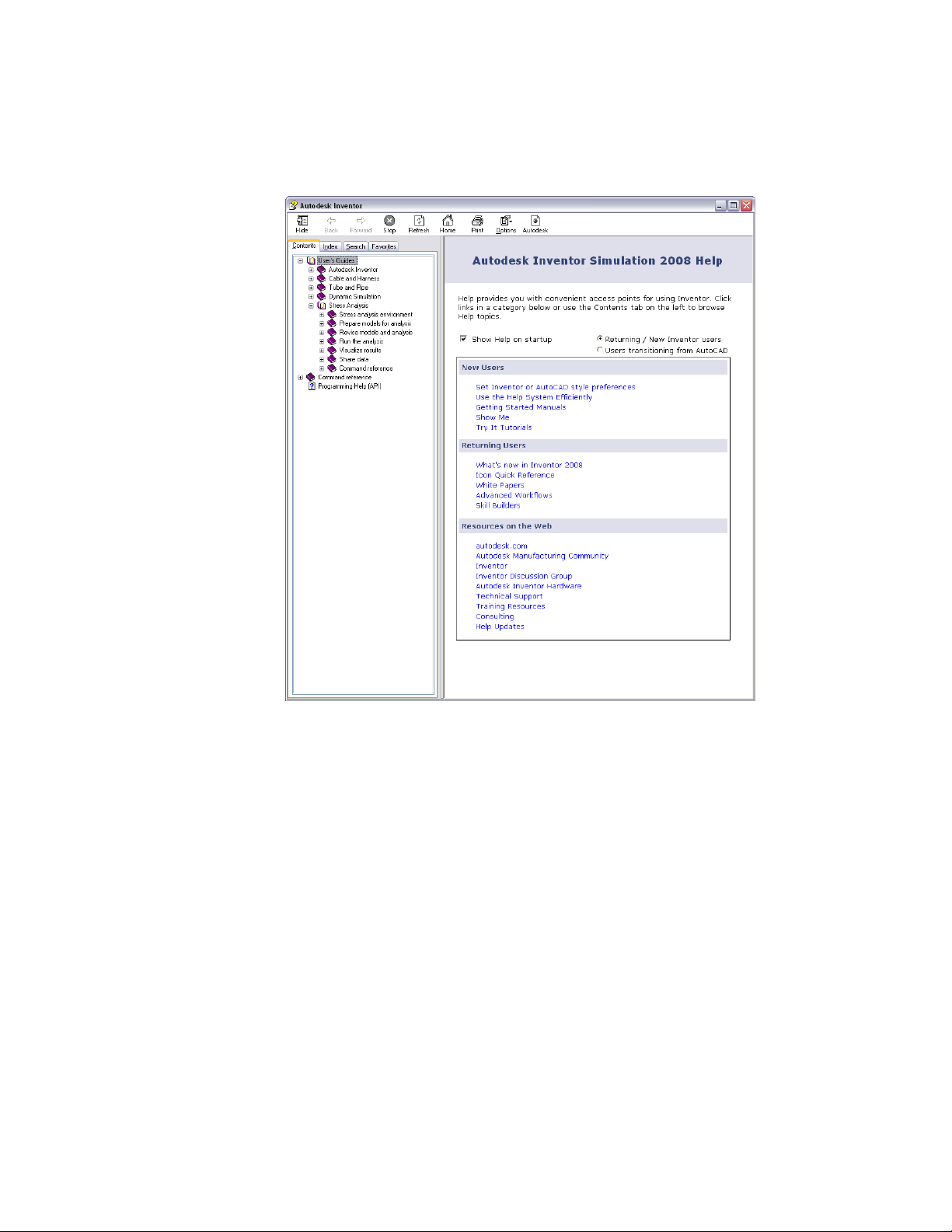
Using Help

®

As you work, you may need additional information about the task you are
performing. The Help system provides detailed concepts, procedures, and
reference information about every feature in the Autodesk Inventor Simulation
Simulation modules as well as the standard Autodesk Inventor Simulation
features.

To access the Help system, use one of the following methods:

■ Click Help ➤ Help Topics, and then use the Table of Contents to navigate

to Stress Analysis topics.

■ Press F1 for Help with the active operation.

■ In any dialog box, click the ? icon.

■ In the graphics window, right-click, and then click How To. The How To

topic for the current tool is displayed.

4 | Chapter 1 Get Started With Stress Analysis

Using Stress Analysis Tools

Autodesk Inventor Simulation Stress Analysis provides tools for determining
structural design performance directly on your Autodesk Inventor Simulation
model. Autodesk Inventor Simulation Stress Analysis includes tools to place
loads and constraints on a part and calculate the resulting stress, deformation,
safety factor, and resonant frequency modes.

Enter the stress analysis environment in Autodesk Inventor Simulation with
an active part.

With the stress analysis tools, you can:

■ Perform a stress or frequency analysis of a part.

Using Stress Analysis Tools | 5

■ Apply a force, pressure, bearing, moment, or body load to vertices, faces,

or edges of the part, or apply a motion load directly to a part.

■ Apply fixed or non-zero displacement constraints to the model.

■ Evaluate the impact of multiple parametric design changes.

■ View the analysis results in terms of equivalent stress, minimum and

maximum principal stresses, deformation, safety factor, or resonant
frequency modes.

■ Add or suppress features such as gussets, fillets or ribs, re-evaluate the

design, and update the solution.

■ Animate part through various stages of deformation, stress, safety factor,

and frequencies.

■ Generate a complete and automatic engineering design report that can be

saved in HTML format.

Understanding the Value of Stress Analysis

Performing an analysis of a mechanical part in the design phase can help you
bring a better product to market in less time. Autodesk Inventor Simulation
Stress Analysis helps you:

■ Determine if the part is strong enough to withstand expected loads or

vibrations without breaking or deforming inappropriately.

■ Gain valuable insight at an early stage when the cost of redesign is small.

■ Determine if the part can be redesigned in a more cost-effective manner

and still perform satisfactorily under expected use.

Stress analysis, for this discussion, is a tool to understand how a design will
perform under certain conditions. It might take a highly trained specialist a
great deal of time performing what is often called a detailed analysis to obtain
an exact answer with regard to reality. What is often as useful to help predict
and improve a design is the trending and behavioral information obtained
from a basic or fundamental analysis. Performing this basic analysis early in
the design phase can substantially improve the overall engineering process.

Here is an example of stress analysis use: When designing bracketry or single
piece weldments, the deformation of your part may greatly affect the alignment
of critical components causing forces that induce accelerated wear. When

6 | Chapter 1 Get Started With Stress Analysis

evaluating vibration effects, geometry plays a critical role in the resonant
frequency of a part. Avoiding or, in some cases, targeting critical resonant
frequencies literally is the difference between part failure and expected part
performance.

For any analysis, detailed or fundamental, it is vital to keep in mind the nature
of approximations, study the results, and test the final design. Proper use of
stress analysis greatly reduces the number of physical tests required. You can
experiment on a wider variety of design options and improve the end product.

To learn more about the capabilities of Autodesk Inventor Simulation Stress
Analysis, view online demonstrations and tutorials, or see how to run analysis
on Autodesk Inventor Simulation assemblies, visit

http://www.ansys.com/autodesk.

Understanding How Stress Analysis Works

Stress analysis is done using a mathematical representation of a physical system
composed of:

■ A part (model).

■ Material properties.

■ Applicable boundary conditions and loads, referred to as preprocessing.

■ The solution of that mathematical representation (solving).

To find a solution, the part is divided into smaller elements. The solver
adds up the individual behaviors of each element to predict the behavior
of the entire physical system.

■ The study of results of that solution, referred to as post-processing.

Analysis Assumptions

The stress analysis provided by Autodesk Inventor Simulation is appropriate
only for linear material properties where the stress is directly proportional to
the strain in the material (meaning no permanent yielding of the material).
Linear behavior results when the slope of the material stress-strain curve in
the elastic region (measured as the Modulus of Elasticity) is constant.

Understanding How Stress Analysis Works | 7

The total deformation is assumed to be small in comparison to the part
thickness. For example, if studying the deflection of a beam, the calculated
displacement must be less than the minimum cross-section of the beam.

The results are temperature-independent. The temperature is assumed not to
affect the material properties.

The CAD representation of the physical model is broken down into small
pieces (think of a 3D puzzle). This process is called meshing. The higher the
quality of the mesh (collection of elements), the better the mathematical
representation of the physical model. By combining the behaviors of each
element using simultaneous equations, you can predict the behavior of shapes
that would otherwise not be understood using basic closed form calculations
found in typical engineering handbooks.

The following is a block (element) with well-defined mechanical and modal
behaviors.

In this example of a simple part, the structural behavior would be difficult to
predict solving equations by hand.

8 | Chapter 1 Get Started With Stress Analysis

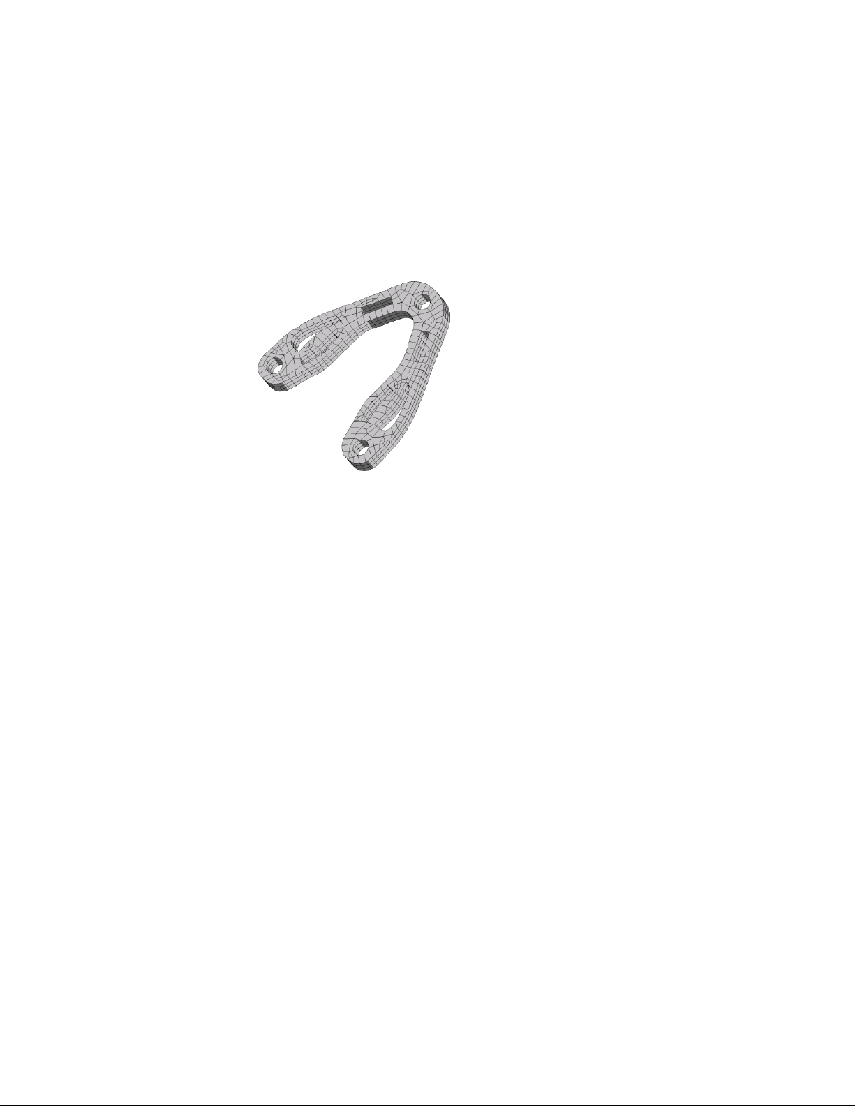
Here, the same part is broken into small blocks (meshed into elements), each
with well-defined behaviors capable of being summed (solved) and easily
interpreted (post-processed). For sheet metal, a special element type is used.
It is assumed that the model is thin in one direction relative to the size of the
other dimensions. The model has identical topologies on the top and bottom
and has only one topology through the thickness of the model.

Interpreting Results of Stress Analysis

The output of a mathematical solver is generally a substantial quantity of raw
data. This quantity of raw data would normally be difficult and tedious to
interpret without the data sorting and graphical representation traditionally
referred to as post-processing. Post-processing is used to create graphical
displays that show the distribution of stresses, deformations, and other aspects
of the model. Interpretation of these post-processed results is the key to
identifying:

■ Areas of potential concern as in weak areas in a model.

■ Areas of material waste as in areas of the model bearing little or no load.

■ Valuable information about other model performance characteristics, such

as vibration, that otherwise would not be known until a physical model
is built and tested (prototyped).

The results interpretation phase is where the most critical thinking must take
place. You compare the results (such as the numbers versus color contours,
movements) with what is expected. You determine if the results make sense,
and explain the results based on engineering principles. If the results are other

Interpreting Results of Stress Analysis | 9

than expected, evaluate the analysis conditions and determine what is causing
the discrepancy.

Equivalent Stress

Three-dimensional stresses and strains build up in many directions. A common
way to express these multidirectional stresses is to summarize them into an
Equivalent stress, also known as the von-Mises stress. A three-dimensional
solid has six stress components. If material properties are found experimentally
by an uniaxial stress test, then the real stress system is related by combining
the six stress components to a single equivalent stress.

Maximum and Minimum Principal Stresses

According to elasticity theory, an infinitesimal volume of material at an
arbitrary point on or inside the solid body can be rotated such that only normal
stresses remain and all shear stresses are zero. When the normal vector of a
surface and the stress vector acting on that surface are collinear, the direction
of the normal vector is called principal stress direction. The magnitude of the
stress vector on the surface is called the principal stress value.

Deformation

Deformation is the amount of stretching that an object undergoes due to the
loading. Use the deformation results to determine where and how much a
part will bend, and how much force is required to make it bend a particular
distance.

Safety Factor

All objects have a stress limit depending on the material used, which is referred
to as material yield. If steel has a yield limit of 40,000 psi, any stresses above
this limit result in some form of permanent deformation. If a design is not
supposed to deform permanently by going beyond yield (most cases), then
the maximum allowable stress in this case is 40,000 psi.

10 | Chapter 1 Get Started With Stress Analysis

A factor of safety can be calculated as the ratio of the maximum allowable
stress to the equivalent stress (von-Mises) and must be over 1 for the design
to be acceptable. (Less than 1 means there is some permanent deformation.)

Factor of safety results immediately points out areas of potential yield, where
equivalent stress results always show red in the highest area of stress, regardless
of how high or low the value. Since a factor of safety of 1 means the material
is essentially at yield, most designers strive for a safety factor of between 2 to
4 based on the highest expected load scenario. Unless the maximum expected
load is frequently repeated, the fact that some areas of the design go into yield
does not always mean the part will fail. Repeated high load may result in a
fatigue failure, which is not simulated by Autodesk Inventor Simulation Stress
Analysis. Always, use engineering principles to evaluate the situation.

Frequency Modes

Use vibration analysis to test a model for:

■ Its natural resonant frequencies (for example, a rattling muffler during idle

conditions, or other failures)

■ Random vibrations

■ Shock

■ Impact

Each of these incidences may act on the natural frequency of the model,
which, in turn, may cause resonance and subsequent failure. The mode shape
is the displacement shape that the model adopts when it is excited at a
resonant frequency.

Frequency Modes | 11

12

Analyze Models

2

Once your model is defined, define the loads and constraints for the condition you want to
test, and then perform an analysis of the model. Use the stress analysis environment to prepare
your model for analysis, and then run the analysis.

This chapter explains how to define loads, constraints, and parameters, and run your analysis.

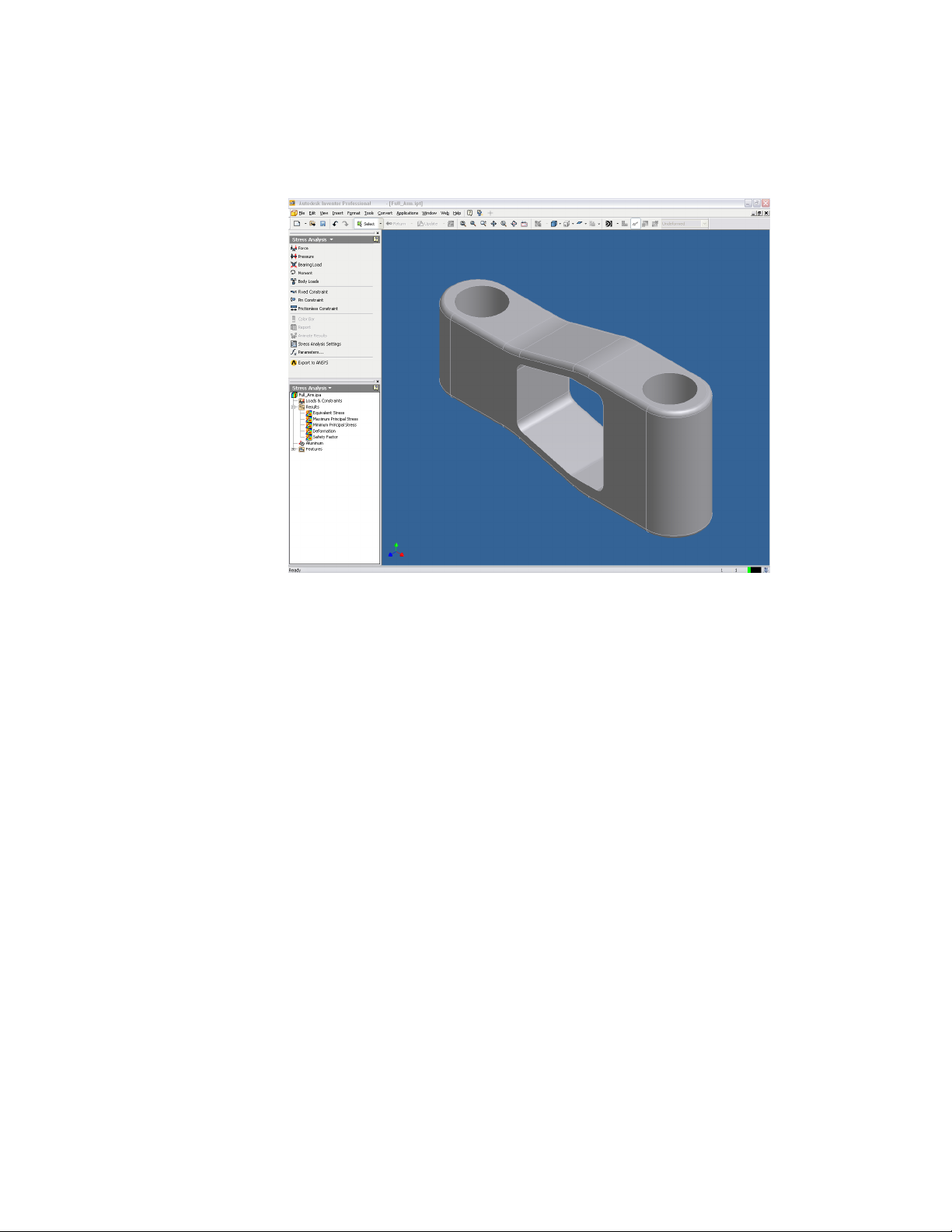
Working in the Stress Analysis Environment

Use the stress analysis environment to analyze your part design and evaluate
different options quickly. You can analyze a part model under different
conditions using various materials, loads, and constraints (or boundary
conditions), and then view the results. You have a choice of performing a stress
analysis, or a resonant frequency analysis with associated mode shapes. After
viewing and evaluating the results, you can change your model and rerun the
analysis to see what effect your changes produced.

You can enter the stress analysis environment from the part and sheet metal
environments.

Enter the stress analysis environment

1 Start with the part or sheet metal environment active.

2 Click Applications ➤ Stress Analysis.

The Stress Analysis panel bar displays.

13

Loads and constraints are listed under Loads & Constraints in the browser. If
you right-click a load or constraint in the browser, you can:

■ Edit the item. The dialog box for that item opens so that you can make

changes.

■ Delete the item.

To rename an item in the browser, click it, enter a new name, and then press
ENTER.

Running Stress Analysis

Once you build or load a part, you can run an analysis to evaluate it for its
intended use. You can perform either a stress analysis or a resonant frequency
analysis of your part under defined conditions. Use the same workflow steps
in either analysis.

The following are the basic steps to perform a stress or resonant frequency
analysis on a part design.

14 | Chapter 2 Analyze Models

Workflow: Perform a typical analysis

1 Enter the stress analysis environment.

2 Verify that the material used for the part is suitable, or select one.

3 On the Stress Analysis panel bar, select the type of load to apply. The

choices are Force, Pressure, Bearing Load, Moment, Body Load, Motion
load (for a part exported from Dynamic Simulation), or Fixed Constraint.

4 On the model, select the faces, edges, or vertices where you want to apply

the load.

5 Enter the load parameters (for example, on the Force dialog box, enter

the magnitude and direction). Numerical parameters can be entered as
numbers or equations that contain user-defined parameters.

6 Repeat steps 3 through 5 for each load on the part.

7 Apply constraints to the model.

8 Change stress analysis environment settings as needed.

9 Modify or add parameters as needed.

10 Start the analysis.

11 View the results.

12 Change the model and reanalyze it until you simulate the appropriate

behavior.

Verifying Material

The first step is to verify that your model material is appropriate for stress
analysis. When you select Stress Analysis, Autodesk® Inventor™ checks the
material defined for your part. If the material is suitable, it is listed in the
Stress Analysis browser. If it is not suitable, a dialog box is displayed so that
you can select a new material.

Verifying Material | 15

You can cancel this dialog box and continue setting up your stress analysis.
However, when you attempt a stress analysis update, this dialog box is
displayed so you can select a valid material before running the analysis.

If the yield strength or density are zero, you cannot perform an analysis.

Once you select a suitable material, click OK.

Applying Loads

The first step in preparing your model for analysis is applying one or more
loads to the model.

Workflow: Apply loads for analysis

1 Select the type of load you want to apply.

2 Select the geometry of the model where the load is applied.

3 Enter the required information for that load.

You can apply as many loads as you need. As you apply them, the loads are
listed in the browser under Loads & Constraints. Once you define a load, you
can edit it by right-clicking it, and then selecting Edit from the menu.

Select and apply a load

1 In the stress analysis environment, Stress Analysis panel bar, click Force.

16 | Chapter 2 Analyze Models

After you select Force, you define the force on the Force dialog box.

2 Click faces, edges, or vertices on the part to select them. Use CTRL-click

to remove a feature from the selection set.

Once you select an initial feature, your selection is limited to features of
the same type (only faces, only edges, only vertices). The location arrow
turns white.

3 Click the direction arrow to set the direction of the force. You can set the

direction normal to a face or work plane, or along an edge or work axis.

Applying Loads | 17

When the force location is a single face, the direction is automatically
set to the normal of the face, with the force pointing to the outside of
the part.

4 To reverse the direction of the force, click the Flip Direction button.

5 Enter the magnitude of the force.

6 To specify the force components, click the More button to expand the

dialog box, and then select the check box for Use Components.

7 Enter either a numerical force value or an equation using defined

parameters. The default value is 100 in the unit system defined for the
part.

8 Click OK.

An arrow is displayed on the model indicating the direction and location
of the force.

You follow a similar procedure for each of the different load types.

18 | Chapter 2 Analyze Models

This table summarizes information about each load type:

Load-Specific InformationLoad

Force

Pressure

Bearing
Load

Moment

Body Loads

Applying Constraints

Apply a force to a set of faces, edges, or vertices. When the
force location is a face, the direction is automatically set to
the normal of the face, with the force pointing to the inside
of the part. Define the direction planar faces, straight edges,
and axes.

Pressure is uniform and acts normal to the surface at all loca­tions on the surface. Apply pressure only to faces.

Apply a bearing load only to cylindrical faces. By default, the
applied load is along the axis of the cylinder and the direction
of the load is radial.

Apply a moment only to faces. Define direction planar faces,
straight edges, two vertices, and axes.

Select a direction from the Earth Standard Gravity list to apply
gravity. Select the Enable check box under Acceleration or
Rotational Velocity. You can only apply one body load per
analysis.

After you define your loads, specify the constraints on the geometry of the
part. You can apply as many constraints as you need. The defined constraints
are listed in the browser under Loads & Constraints. After you define a
constraint, you can edit it by right-clicking it, and then selecting Edit from
the menu.

Select and apply a constraint

1 On the Stress Analysis panel bar, click Fixed Constraint, Pin Constraint,

or Frictionless Constraint.

2 In the graphics window, select a set of faces, edges, or vertices to constrain.

The location arrow turns white.

Applying Constraints | 19

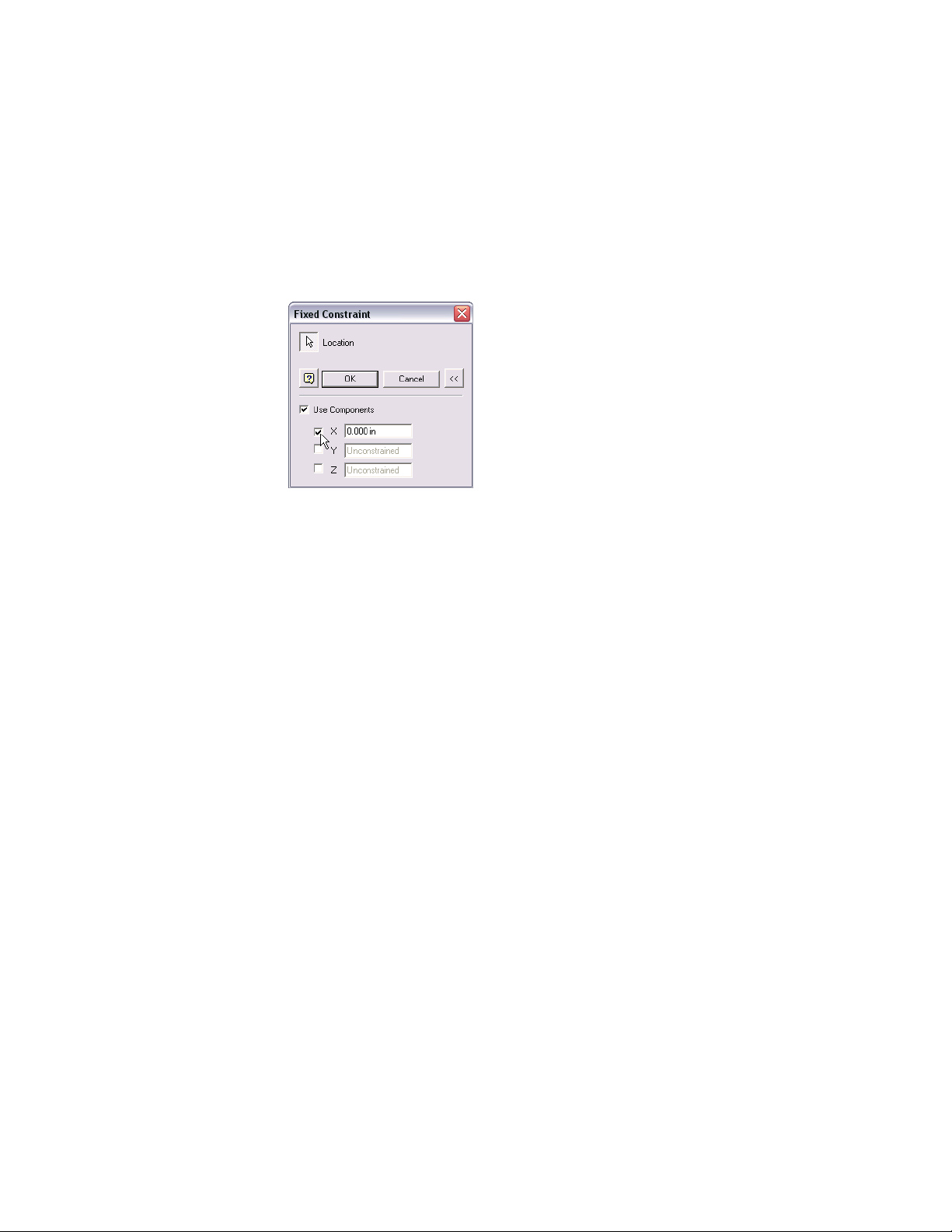
3 Click the More button to specify a fixed displacement for the constraint,

if needed. Check Use Components, and then check the box next to the
global axis label (X, Y, or Z) along which the displacement occurs.

You can use parameters and negative values. Use Components to specify
a non-zero displacement that can be used as a load.

4 Click OK.

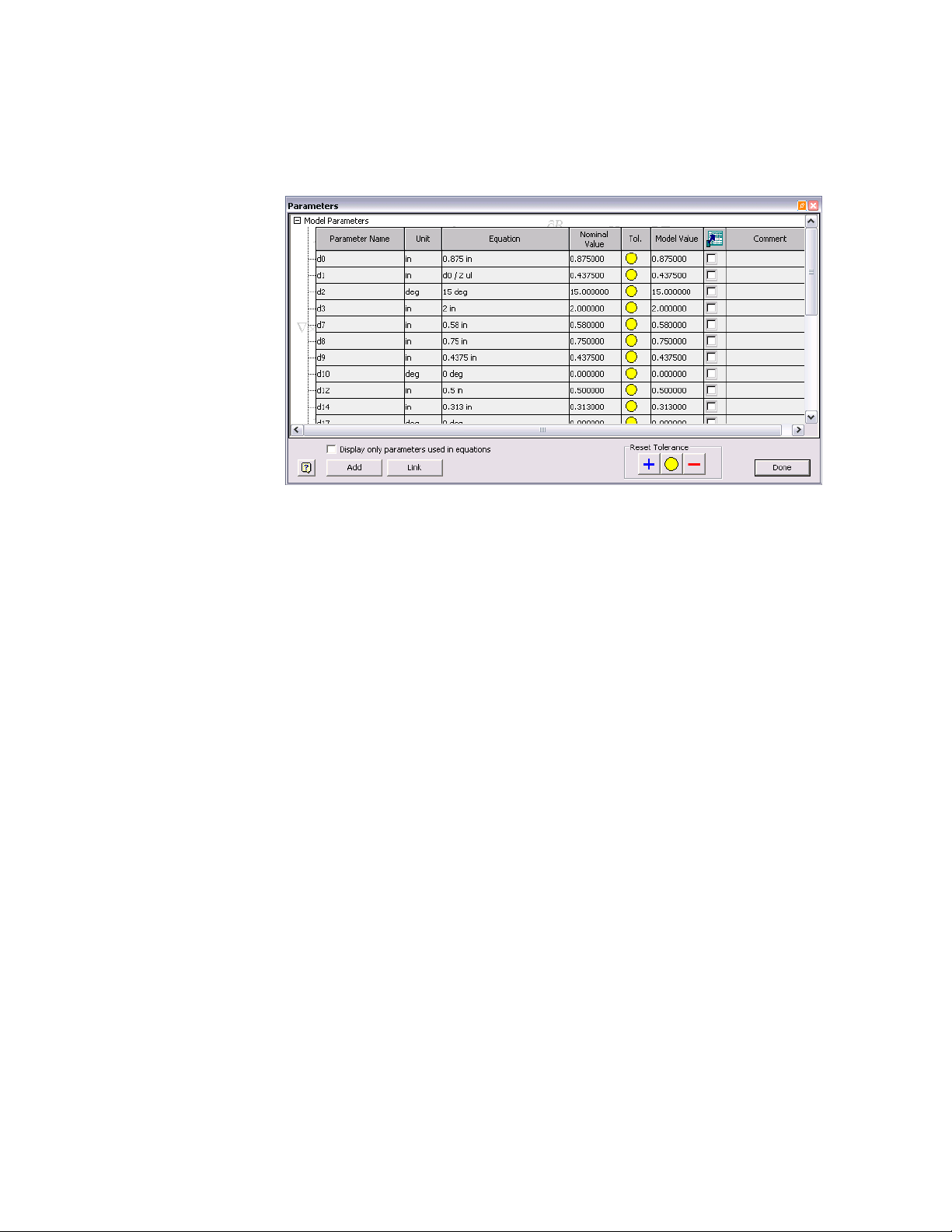
Setting Parameters

When you define loads and constraints for a part, the values you enter
(magnitudes, vector components, and so on) are stored as parameters in
Inventor. It automatically generates the parameter names. For example, load
parameters are labeled dn, where d0 is the first load created, d1 the second
load, and so on.

Load magnitude and constraint displacement values can be entered as
equations when you are defining them. Or, after defining the loads and
constraints, select Parameters from the stress analysis panel bar. On the
Parameters dialog box, enter equations for any of the load or constraint
parameters.

20 | Chapter 2 Analyze Models

You can define and edit parameters at any time, either during part modeling,
analysis setup, or post-processing. If you change the parameters associated
with a load or constraint after a solution is obtained, the Update command
is enabled so you can run a new solution.

You cannot delete the system-generated parameters, although they are deleted
automatically if their associated loads or constraints are deleted. You also
cannot delete parameters that are currently used by a system-generated
parameter.

Feature Suppression Tracking

When conducting analysis studies, you may need to tailor portions of a model
to allow for a more efficient analysis. Generally, this technique involves
removing geometrically small features which only complicated the mesh,
without significant effects to the final result.

Setting Solution Options

Before starting your solution, set the analysis type and mesh relevance for the
analysis, and then specify whether to create new analysis file. Select Stress
Analysis Settings from the stress analysis panel bar to open the dialog box.
When you finish setting the options, click OK to commit them.

Feature Suppression Tracking | 21

Setting Analysis Type

Before starting your solution, on the Settings dialog box, Analysis Type, select
Stress Analysis, Modal Analysis (to perform resonant frequency analysis) or
Both (to run a stress analysis and a prestressed modal analysis of your part).

Setting Mesh Control

There are two meshing model types: standard solid model and optimized thin
model. For a part, the default is standard solid model. It can be meshed in all
X, Y, and Z directions. The default meshing model for sheet metal is optimized
thin model. It is assumed that the model is thin in one direction relative to
the size of the other dimensions, has identical topologies on the top and
bottom, and has only one topology through the thickness of the model. On
the Settings dialog box, move the Mesh Relevance slider to set the size of your
mesh. The default value of zero is an average mesh. Setting the slider to 100
causes a fine mesh to be used. It gives you a highly accurate result, but causes
the solution to take a longer time. Setting the slider to -100 gives you a coarse
mesh, which solves quickly, but may contain significant inaccuracies. The
Mesh Relevance and Result Convergence only work for the standard solid

22 | Chapter 2 Analyze Models

model. You can see the mesh that to use at a particular setting by clicking
Preview Mesh.

Select the Results Convergence check box to allow Autodesk Inventor
Simulation to improve the mesh adaptively.

Multi-Step Motion

Move Active Part

Create OLE Link to
Result Files

Simulates the position for a part applied motion load
from Dynamic Simulation in an assembly.

Moves the active part and fixes other non-active parts
with different time steps.

Fixes the active part and moves other non-active parts.Move Assembly

Keeps the relationship between a part document and
other stress analysis files.

Obtaining Solutions

After you complete all the required steps, the Stress Analysis Update command
on the Standard toolbar is active. Select it to start the solution.

The Solutions Status dialog box is displayed while the solution is in progress.
During the solution, Autodesk Inventor Simulation is unavailable. Once the
solution finishes, the results are displayed graphically.

For information about reviewing the results of your solution, see View Results
on page 25.

Running Modal Analysis

In addition to the stress analysis, you can perform a resonant frequency (modal)
analysis to find the frequencies at which your part vibrates, and the mode
shapes at those frequencies. Like stress analysis, modal analysis is available in
the stress analysis environment.

You can do a resonant frequency analysis independent of a stress analysis.
You can do a frequency analysis on a prestressed structure, in which case you
can define loads on the part before the analysis. You can also find the resonant
frequencies of an unconstrained part.

Your initial steps must be the same as for stress analysis. Refer to the
instructions in Running Stress Analysis on page 14 to set up your loads,
constraints, parameters, and solution options.

Obtaining Solutions | 23

Workflow: Run a modal analysis

1 Enter the stress analysis environment.

2 Verify that the material used for the part is suitable, or select one.

3 Apply any loads (optional).

4 Apply the necessary constraints (optional).

5 Before starting the solution, on the Settings dialog box, Analysis Type

section, select Modal Analysis.

Selecting Both runs a stress analysis and a modal analysis of your part.
Selecting a modal analysis with a load applied produces a prestressed
modal solution.

6 Click OK.

The results for the first six frequency modes are inserted under the Modes
folder in the browser. For an unconstrained part, the first six frequencies
are essentially zero.

7 To change the number of frequencies displayed or limit the range of

frequency results returned, right click the Modes folder, and then select
Options.

The Frequency Options dialog box is displayed. Enter the maximum
number of modes to find, or the range of frequencies to which you want
to limit the results set.

After you complete all the required steps, the Stress Analysis Update
command on the standard toolbar is active.

8 Select Stress Analysis Update to start the solution.

The Solutions Status dialog box is displayed while the solution is in
progress. Once the solution finishes, the results are available for viewing.

24 | Chapter 2 Analyze Models

View Results

3

After analyzing your model under the stress analysis conditions that you defined, you can
visually observe the results of the solution.

This chapter describes the how to interpret the visual results of your stress analyses.

Using Results Visualization

Use results visualization to see how your part responds to the loads and
constraints you apply to it. You can visualize the magnitude of the stresses that
occur throughout the part, the deformation of the part, and the stress safety
factor. For modal analysis, you can visualize the resonant frequency modes.

Enter results visualization

1 Start in the stress analysis environment. Open a part or sheet metal part

that was analyzed previously, or complete the required steps in your current
analysis.

2 On the standard toolbar, click the Stress Analysis Update tool.

The color bar displays in the graphics window.

Post-processing commands are enabled on the standard toolbar, and the display
mode shifts to stepped contours.

25

To view the different results sets, double-click them in the browser. While
viewing the results, you can:

■ Change the color bar to emphasize the stress levels that are of concern.

■ Compare the results to the undeformed geometry.

■ View the mesh used for the solution.

Use the normal view controls to manipulate the model for a 3-dimensional
view of the results.

To change any model parameters, return to part modeling, and then return
to stress analysis and update the solution.

Editing the Color Bar

The color bar shows you how the contour colors correspond to the stress
values or displacements calculated in the solution. You can edit the color bar
to set up the color contours so that the stress/displacement is displayed in a
way that is meaningful to you.

26 | Chapter 3 View Results

Edit the color bar

1 Click Color Bar on the Stress Analysis panel bar.

By default, the maximum and minimum values shown on the color bar
are the maximum and minimum result values from the solution. You
can edit the extreme maximum and minimum values, and the values at
the edges of the bands.

2 To edit the maximum and minimum critical threshold values, click the

Automatic check box to clear the selection, and then edit the values in
the text box. Click Apply to complete the change.

To restore the default maximum and minimum critical threshold values,
select Automatic, and then click Apply.

The levels are initially divided into seven equivalent sections, with default
colors assigned to each section. You can select the number of contour
colors in the range of 1 to 12.

3 To increase or decrease the number of colors, click the Increase

Colors and Decrease Colors buttons. You can also enter the number of
colors you want in the text box.

4 Click the Invert Colors check box to reverse the sequence of colors

displayed in the color bar.

5 You can view the result contours in different colors or in shades

of gray. To view result contours on the grayscale, click Grayscale under
Color.

NOTE It does not work for safety factor.

6 By default, the color bar is positioned in the upper-left corner. Select an

appropriate option under Position to place the color bar at a different
location.

7 Under Size, select an appropriate option to resize the color bar, and then

click Apply.

The color bar preferences such as color, position, and size are applied to
all of the result types.

The Maximum and Minimum threshold values, number of colors and
Invert colors preferences are applied only to the selected result type.

Editing the Color Bar | 27

Reading Stress Analysis Results

When the analysis is complete, you see the results of your solution. If you did
a stress analysis or specified that both types of analyses to do, you initially see
the equivalent stress results set displayed. If your initial analysis is a resonant
frequency analysis (without a stress analysis), you see the results set for the
first mode. To view a different results set, double-click that results set in the
browser pane. The currently viewed results set has a check mark displayed
next to it in the browser. You always see the undeformed wireframe of the
part when you are viewing results.

Interpreting Results Contours

The contour colors displayed in the results correspond to the value ranges
shown in the legend. In most cases, results displayed in red are of most interest,
either because of their representation of high stress or high deformation, or
a low factor of safety. Each results set gives you different information about
the effect of the load on your part.

Equivalent Stress

Equivalent stress results use color contours to show you the stresses calculated
during the solution for your model. The deformed model is displayed. The
color contours correspond to the values defined by the color bar.

Maximum Principal Stress

The maximum principal stress gives you the value of stress that is normal to
the plane in which the shear stress is zero. The maximum principal stress helps
you understand the maximum tensile stress induced in the part due to the
loading conditions.

28 | Chapter 3 View Results

Minimum Principal Stress

The minimum principal stress acts normal to the plane in which shear stress
is zero. It helps you understand the maximum compressive stress induced in
the part due to the loading conditions.

Deformation

The deformation results show you the deformed shape of your model after
the solution. The color contours show you the magnitude of deformation
from the original shape. The color contours correspond to the values defined
by the color bar.

Safety Factor

Safety factor shows you the areas of the model that are likely to fail under
load. The color contours correspond to the values defined by the color bar.

Frequency Modes

You can view the mode plots for the number of resonant frequencies that you
specified in the solution. The modal results appear under the Modes folder in
the browser. When you double-click a frequency mode, the mode shape is
displayed. The color contours show you the magnitude of deformation from
the original shape. The frequency of the mode shows in the legend. It is also
available as a parameter.

Animate Results

Use the Animate Results tool to visualize the part through various stages of
deformation. You can also animate stress, safety factor, and deformation under
frequencies.

Animate Results | 29

Setting Results Display Options

While viewing your results, you can use the following commands located on
the Stress Analysis Standard toolbar to modify the features of the results display
for your model.

Used toCommand

Maximum

Minimum

Condition

Element Visi­bility

Turns on and off the display of the point of maximum result
in the mode.

Turns on and off the display of the point of minimum result
in the model.

Turns on or off the display of the load symbols on the part.Boundary

Displays the element mesh used in the solution in conjunction
with the result contours.

Use the Deformation Style menu to change the deformed shape exaggeration.
Selecting Actual shows you the deformation to scale. Since the deformations
are often small, the various automatic options exaggerate the scale so that the
shape of the deformation is more pronounced.

Use the Display Settings menu to set the contour style to stepped, smooth, or
no contours. If you turn off the contours, the mesh is displayed for your
deformed part. If you have Element Visibility on, the mesh elements are
displayed. Otherwise, a solid, gray mesh is displayed. The legend shows while
contours are off.

The values of all of the display options for each results set are saved for that
results set.

30 | Chapter 3 View Results

Revise Models and Stress Analyses

After you run a solution for your model, you can evaluate how changes to the model or
analysis conditions will affect the results of the solution.

This chapter explains how to change solution conditions on the part and rerun the solution.

4

Changing Model Geometry

After you run an analysis on your model, you can change the design of your
model. Rerun the analysis to see the effects of the changes.

Edit a design and rerun analysis

1 Return to part modeling by clicking Applications ➤ Part, or Model on the

browser menu.

The part modeling toolbars and browser are displayed, and the graphics
window changes back to the solid undeformed part.

2 Click Last Displayed Stress Result to turn on the display of the last

results set.

Viewing the results of your solution as you edit the initial geometry can
give you an insight as to which dimension to edit to get results closer to
your intent.

3 In the browser, select the feature that you want to edit. It highlights on

the wireframe.

31

4 In the browser, right-click a sketch for the feature that you want to edit.

Click Visibility to make the sketch visible on the model.

5 Double-click the dimension that you want to change, enter the new value

in the text box, and then click the green check mark. The sketch updates.

6 Click Applications ➤ Stress Analysis.

7 On the Standard toolbar, click Stress Analysis Update.

After you update the stress analysis, the load symbols relocate if the feature
that they were associated with moved as a result of the geometry change. The
direction of the load does not change, even if the feature associated with the
load changes orientation.

Changing Solution Conditions

After you run an analysis on your model, you can change the conditions under
which the solution was obtained. Rerun the analysis to see effects of the
changes. You can edit the loads and constraints you defined, add new loads
and constraints, or delete loads and constraints. You can also change the
relevance of your mesh or the analysis type. To change your solution
conditions, enter the stress analysis environment if you are not already in it.

Delete a load or constraint

■ In the browser, right-click a load or constraint, and then select Delete from

the menu.

Add a load or constraint

■ On the panel bar, select the command and follow the same procedure you

used to create your initial loads and constraints.

Edit a load or constraint

1 In the browser, right-click a load or constraint, and then select Edit from

the menu.

The same dialog box you used to create the load or constraint is displayed.
The values on the dialog box are the current values for that load or
constraint.

32 | Chapter 4 Revise Models and Stress Analyses

2 Click the location arrow on the left side of the dialog box to enable feature

picking.

You are initially limited to selecting the same type of feature (face, edge,
or vertex) that is currently used for the load or constraint.

To remove any of the current features, control-click them. If you remove
all of the current features, your new selections can be of any type.

3 Click the white Direction arrow to change the direction of the load.

4 Click the Flip Direction button to reverse the direction, if needed.

5 Change any values associated with the load or constraint.

6 Click OK to apply the load or constraint changes.

Hide a load symbol

■ On the toolbar, click the Boundary Condition display button.

The load symbols are hidden.

Redisplay a load symbol

■ On the toolbar, click the Boundary Condition display button again.

The load symbols redisplay.

Temporarily display load symbols

■ In the browser, pause the cursor over the Loads & Constraints folder

or a particular load.
The load symbols display.

NOTE If you edit a load while the load symbols are hidden, the symbols for
all the loads display. They remain displayed after the editing is complete.

Change the mesh relevance

1 On the Stress Analysis panel bar, click Stress Analysis Settings.

2 On the Settings dialog box, move the slider to set the relevance of your

mesh.

3 Click Preview Mesh to view the mesh at a particular setting.

Changing Solution Conditions | 33

The preview mesh is shown on the undeformed shaded view of your part.

Change the analysis type

1 On the Stress Analysis panel bar, click Stress Analysis Settings.

2 On the Settings dialog box, Analysis Type menu, select the new analysis

type.

If you choose Stress Analysis or Modal Analysis, only the results sets for
the selected analysis type are displayed in the browser. Any previously
obtained results sets are removed.

Change the element type for sheet metal

1 On the Stress Analysis panel bar, click Stress Analysis Settings.

2 On the Setting dialog box, select Standard Solid Model.

Updating Results of Stress Analysis

After you change any of the solution conditions, or if you edit the part
geometry, the current results are invalid. A lightning bolt symbol on the results
icons indicates the invalid status. The Stress Analysis Update item becomes
active on Standard toolbar.

Update stress analysis results

■ On the Standard toolbar, click Stress Analysis Update.

New results generate based on your revised solution conditions.

34 | Chapter 4 Revise Models and Stress Analyses

Generate Reports

5

Once you run an analysis on a part, you can generate a report that provides you with a written
record of the analysis environment and results.

This chapter tells you how to generate a report for an analysis and interpret the report, and
how to save and distribute the report.

Running Reports

After you run a stress analysis on a part, you can save the details of that analysis
for future reference. Use the Report command to save all the analysis conditions
and results in HTML format for easy viewing and storage.

Generate a report

1 Set up and run an analysis for your part.

2 Set the zoom and view orientation to illustrate the analysis results. The

view you choose is the view used in the report.

3 On the panel bar, click Report to create a report for the current analysis.

When it finishes, a browser window containing the report is displayed.

4 Save the report for future reference using the browser Save As command.

Interpreting Reports

The report contains a summary, introduction, scenario, and appendices.

35

Summary

The summary contains an overview of the files used for the analysis and the
analysis conditions and results.

Introduction

The introduction describes the contents of the report and how to use them
in interpreting your analysis.

Scenario

The scenario gives details about the various analysis conditions.

Model

The model section contains:

■ A description of the mesh relevance, and number of nodes and elements

■ A description of the physical characteristics of the model

Environment

The environment section contains:

■ Loading conditions and constraints

Solution

■ Equivalent stress

■ Maximum and minimum principal stresses

■ Deformation

36 | Chapter 5 Generate Reports

■ Safety factor

■ Frequency response results

Appendices

Appendices include labeled scenario figures, which show the contours for the
different results sets. The sets include equivalent stress, maximum and
minimum principal stresses, deformation, safety factor, and mode shapes

Saving and Distributing Reports

The report is generated as a set of files to view in a Web browser. It includes
the main HTML page, style sheets, generated figures, and other files listed at
the end of the report.

Saving Reports

Use your browser Save As command to save all of the report files into a folder
of your choosing. Recent versions of Microsoft Internet Explorer® give you
the option of opening and saving your report in Microsoft® Word.

Be careful when you save a report into a folder where you previously saved a
copy of the same report. It is possible to end up with files in the directory that
were used by the previous version of the report, but are not used by the current
version. To avoid confusion, it is best to use a new folder for each version of
a report, or to delete all of the files in a folder before reusing it.

Printing Reports

Use your Web browser Print command to print the report as you would any
Web page.

Appendices | 37

Distributing Reports

To make the report available from a Web site, move all the files associated
with the report to your Web site. Distribute a URL that points to the main
page of the report, the first file listed in the table.

38 | Chapter 5 Generate Reports

Manage Stress Analysis Files

Running a stress analysis in Autodesk® Inventor™ Simulation creates a separate file that
contains the stress analysis information. In addition, the part file is modified to indicate the
presence of a stress file and the name of the file.

This chapter explains how the files are interdependent, and what to do if the files become
separated.

6

Creating and Using Analysis Files

You can run a stress analysis by creating a part in Autodesk Inventor Simulation,
and then setting up your stress analysis conditions. You can also load a part
that you previously created, on which you have not yet run a stress analysis,
and set up your analysis conditions. Once you set up a stress analysis for a part,
when you save the part you also save the stress analysis information for that
part.

Start a new analysis

1 Load an existing part or create a part in the part or sheet metal

environments.

2 Enter the stress analysis environment by clicking Applications ➤ Stress

Analysis.

3 Set up your analysis conditions.

After you set up any stress analysis information, saving your part also saves the
associated stress analysis information in the part file. Stress analysis input and
results information, including loads, constraints, and all results, is also saved

39

in a separate file. The stress analysis file has the same name as your part file,
but uses the extension .ipa. By default, the .ipa file is stored in the same folder
as the .ipt file.

The _structure.rst (for stress analysis) and the _modal.rst (for modal analysis)
files, used to export to ANSYS, are generated after you save. If you select both,
the _strucure.esave and _structure.db files, used to export to ANSYS, are also
generated and stored in a subfolder like the .ipt file.

Understanding File Relationships

Activating the stress analysis environment, and then saving the .ipt file does
not create the analysis files. Add at least one stress analysis update before
Autodesk Inventor Simulation creates the .ipa file.

The analysis files contain information that indicates which .ipt file is associated
with the .ipa file. Multiple .ipt files cannot reference the same .ipa file, and
multiple .ipa files cannot reference the same .ipt file.

The Save Copy As command does not generate a new .ipa file. This means
that the new .ipt file references the same .ipa file as the old .ipt file.

On the Stress Analysis Setting dialog box, use the Create OLE Link to Result
Files option to keep the relationship between the analysis files except for the

.ipa and .ipt files. If the option is checked, the files are necessary to open the
.ipt file.

For more information about the Save Copy As command, see Copying

Geometry Files on page 41 in this chapter.

NOTE An existing .ipa file is not loaded until you activate the stress analysis
environment.

Repairing Disassociated Files

Under certain circumstances, edit the part file without the presence of the .ipa
file. For example, you sent the .ipt file but not the .ipa file to a consultant.
You can edit the part file through the Skip option on the Resolve Link dialog
box.

If you edit the part while the .ipa file is missing, and then try to reassociate
the part with its analysis file, Inventor makes an attempt to update the stress

40 | Chapter 6 Manage Stress Analysis Files

conditions. There is a possibility that errors can occur when you try to
reassociate the files.

Copying Geometry Files

You can create a copy of an .ipt file using the Save Copy As command or your
operating system file copy command. The copy of the .ipt file still references
the original .ipa file.

Resolving File Link Failures

In some cases, the .ipa file might fail to resolve when you try to perform an
analysis of the part. For example, you rename or move the .ipa file, or a vendor
receives a copy of an .ipt file without the associated .ipa file. The .ipa file fails
to resolve and you are prompted with the Resolve Link dialog box.

You can do two things, other than cancel the file open process:

■ Skip the file.

■ Select an existing .ipa file.

Skipping Missing IPA Files

If you select to edit a part even though the .ipa file is missing, you can enter
the stress analysis environment. Create an .ipa file by rerunning the stress
analysis update and saving. You can edit the part document itself. However,
you cannot perform any stress analysis work.

Selecting Existing IPA Files

If the .ipa file is missing, you can select an existing renamed or moved .ipa
file.

Copying Geometry Files | 41

Creating New Analysis Files

To create an .ipa file, click the Stress Analysis Update button on the standard
toolbar and save it. Inventor attempts to create an .ipa file in the default
location using the default name.

If a file exists using this name and location, Inventor checks the .ipa file to
see if it points to the active .ipt file. If it does, the new .ipa file replaces the old
one.

When you create a file, the new .ipa file has boundary conditions that match
the conditions stored in the .ipt file.

Exporting Analysis Files

To run a more complex analysis on your part than Autodesk Inventor
Simulation Stress Analysis can handle, export your current analysis information
to a file that ANSYS WorkBench can import.

Export your information to ANSYS WorkBench

1 After you set up and run an analysis, on the Stress Analysis panel bar,

click Export to ANSYS.

2 Browse to the location where you store your project files.

3 Click Save.

The file is saved using the same name as your part file, with the extension
.dsdb.

You can now import your part and its analysis file into ANSYS WorkBench to
perform more complex analyses.

42 | Chapter 6 Manage Stress Analysis Files

Simulation

Part 2 of this manual presents the getting started information for Autodesk® Inventor
Simulation. This application environment provides tools to predict dynamic performance
and peak stresses before building prototypes.

™

43

44

Get Started with Simulation

About Autodesk Inventor Simulation

Autodesk®Inventor™ Simulation provides tools to simulate and analyze the
dynamic characteristics of an assembly in motion under various load conditions.
You can also export load conditions at any motion state to Stress Analysis in
Autodesk Inventor Simulation to see how parts respond from a structural point
of view to dynamic loads at any point in the range of motion of the assembly.

The dynamic simulation environment works only with Autodesk® Inventor
assembly (.iam) files.

With the dynamic simulation, you can:

■ Have the software automatically convert all mate and insert constraints into

standard joints.

7

™

■ Access a large library of motion joints.

■ Define external forces and moments.

■ Create motion simulations based on position, velocity, acceleration, and

torque as functions of time in joints, in addition to external loads.

■ Visualize 3D motion using traces.

■ Export full output graphing and charts to Microsoft

■ Transfer dynamic and static joints and inertial forces to Autodesk Inventor

Simulation Stress Analysis or ANSYS Workbench.

®

Excel®.

45

■ Calculate the force required to keep a dynamic simulation in static

equilibrium.

■ Convert assembly constraints to motion joints.

■ Use friction, damping, stiffness, and elasticity as functions of time when

defining joints.

■ Use dynamic part motion interactively to apply dynamic force to the

jointed simulation.

■ Use Inventor Studio to output realistic or illustrative video of your

simulation.

Learning Autodesk Inventor Simulation

We assume that you have a working knowledge of the Autodesk Inventor
Simulation interface and tools. If you do not, use the integrated Help for access
to online documentation and tutorials, and complete the exercises in this
manual.

At a minimum, we recommend that you understand how to:

■ Use the assembly, part modeling, and sketch environments and browsers.

■ Edit a component in place.

We also recommend that you have a working knowledge of Microsoft
Windows® XP or Windows® Vista™, and a working knowledge of concepts
for stressing and analyzing mechanical assembly designs.

Using Help

As you work, you may need additional information about the task you are
performing. The Help system provides detailed concepts, procedures, and
reference information about every feature in the Autodesk Inventor Simulation
Simulation modules as well as the standard Autodesk Inventor Simulation
features.

To access Help, use one of the following methods:

■ Click Help ➤ Help Topics. On the Contents tab, click Dynamic Simulation.

46 | Chapter 7 Get Started with Simulation

®

■ In any dialog box, click the ? icon.

Understanding Simulation Tools

Large and complex moving assemblies coupled with hundreds of articulated
moving parts can be simulated. Autodesk Inventor Simulation Simulation
provides:

■ Interactive, simultaneous, and associative visualization of 3D animations

with trajectories; velocity, acceleration, and force vectors; and deformable
springs.

■ Graphic generation tool for representing and post-processing the simulation

output data.

Simulation Assumptions

The dynamic simulation tools provided in Autodesk Inventor Simulation help
in the steps of conception and development and in reducing the number of
prototypes. However, due to the hypothesis used in the simulation, it only
provides an approximation of the behavior seen in real-life mechanisms.

Interpreting Simulation Results

To avoid computations that can lead to a misinterpretation of the results or
incomplete models that cause unusual behavior, or even make the simulation
impossible to compute, be aware of the rules that apply to:

■ Relative parameters

■ Continuity of laws

■ Coherent masses and inertia

Relative Parameters

Autodesk Inventor Simulation Simulation uses relative parameters. For example,
the position variables, velocity, and acceleration give a direct description of

Understanding Simulation Tools | 47

the motion of a child part according to a parent part through the degree of
freedom (DOF) of the joint that links them. As a result, select the initial velocity
of a degree of freedom carefully.

Coherent Masses and Inertia

Ensure that the mechanism is well-conditioned. For example, the mass and
inertia of the mechanism should be in the same order of magnitude. The most
common error is a bad definition of density or volume of the CAD parts.

Continuity of Laws

Numerical computing is sensitive toward incontinuities in imposed laws. Thus,
while a velocity law defines a series of linear ramps, the acceleration is
necessarily discontinuous. Similarly, when using contact joints, it is better to
avoid profiles or outlines with straight edges.

NOTE Using little fillets eases the computation by breaking the edge.

48 | Chapter 7 Get Started with Simulation

Simulate Motion

8

With the dynamic simulation or the assembly environment, the intent is to build a functional
mechanism. Dynamic simulation adds to that functional mechanism the dynamic, real-world
influences of various kinds of loads to create a true kinematic chain.

Understanding Degrees of Freedom

Though both have to do with creating mechanisms, there are some critical
differences between the dynamic simulation and the assembly environment.
The most basic and important difference has to do with degrees of freedom.

By default, components in Autodesk® Inventor™ Simulation have zero degrees
of freedom. Unconstrained and ungrounded components in the assembly
environment have six degrees of freedom.

In the assembly environment, you add constraints to restrict degrees of freedom.
In the dynamic simulation environment, you build joints to create degrees of
freedom.

Understanding Constraints

By default, any constraints that exist in the assembly have no effect on dynamic
simulation.

Open sample files

1 Set your active project to tutorial_files and then open Gate.iam.

2 Save a copy of this assembly. Name the copy Gate-saved.iam. Close Gate.iam

and then open Gate-saved.iam.

49

3 To see how the assembly moves, drag the door.

As you work through the following exercises, save this assembly
periodically.

Converting Assembly Constraints

Notice that the assembly moves just as it did in the assembly environment.
It seems to contradict preceding explanations, however, the motion you see
is borrowed from the assembly environment. Even though you are in Autodesk
Inventor Simulation Simulation, you are not yet running a simulation. Since
a simulation is not active, the assembly is free to move.

Enter the dynamic simulation environment

1 Click Applications ➤ Dynamic Simulation.

The dynamic simulation environment is active.

NOTE If the open assembly was created in Autodesk Inventor Simulation
2008 or later, Automatically Convert Constraint to Standard Joints is selected
in Dynamic Simulation settings by default. Since this assembly was first created
in a previous version of Inventor and saved in Dynamic Simulation,
Automatically Convert Constraints to Standard Joints is unselected by default.
Although this function is powerful and useful, it is not selected currently for
training purposes.

2 At the bottom of the browser, click the Run button on the

Simulation panel.

50 | Chapter 8 Simulate Motion

The Dynamic Simulation browser turns gray and the status slider on the
simulation panel moves, indicating that a simulation is running.

Since we have not created any joints (and have not specified any driving
forces) the assembly is grounded and does not move.

3 If the status slider is still moving, click the Stop button.

Even though the simulation is not running, the simulation mode is still
active.

4 Attempt to drag the Door component. It does not move.

5 On the Dynamic Simulation panel bar, click Activate Construction

Mode at the bottom of the browser.

It exits the simulation mode and returns to the Dynamic Simulation
construction mode. In construction mode, you perform such tasks as
creating joints and applying loads.

Automatically convert assembly constraints

1 On the Dynamic Simulation panel bar, click Dynamic Simulation Settings.

This dialog box now has the Automatically Convert Constraints to
Standard Joints option, which automatically translates certain assembly
constraints to standard joints.

When you open an assembly created in Autodesk Inventor Simulation
2009, Automatically Convert Constraints to Standard Joints is selected
by default. However, since this assembly was created in an earlier version
of Inventor, the default is not selected.

2 On the Dynamic Simulation Settings dialog box, click Automatically

Convert Constraints to Standard Joints.

3 Click Apply.

One welded group and five standard joints are created.

4 In the Dynamic Simulation browser, navigate to the Mobile Groups folder,

and then open the Welded group folder. Notice the two parts that the
software has welded as one step of translating assembly constraints.

5 In the Standard Joints folder, notice the standard joints that the software

has automatically created for you.

Converting Assembly Constraints | 51

6 On the Dynamic Simulation Settings dialog box, remove the check mark

next to Automatically Convert Constraints to Standard Joints.

NOTE Selecting this option deletes all joints already in the assembly.

7 Click OK.

Convert constraints

1 On the Dynamic Simulation panel bar, click Convert Assembly

Constraints.

NOTE Autodesk Inventor Simulation Simulation converts constraints that
have to do with degrees of freedom, such as Mate or Insert, but does not
convert constraints that have to do with position, such as Angle.

2 Select the Door component (3).

3 Select the Pillar component (4).

Assembly constraints that exist between the two parts are listed on the
dialog box. In this case, there are two mate constraints: an axial constraint
between the hinge axes and a face-to-face constraint between the hinge
top and bottom flat faces.

52 | Chapter 8 Simulate Motion

Axial constraint between the hinge axes

Face-to-face constraint between hinge top and bottom flat faces

4 Select the check box next to Mate1: (door:1, pillar:1). It is the axial

constraint.

Converting Assembly Constraints | 53

Notice that the joint type (Cylindrical) is listed in the Joint field and the
animation switches to the Cylindrical Joint animation. Autodesk Inventor
Simulation Simulation automatically selects the appropriate joint needed
for the constraint conversion.

5 Remove the check mark next to Mate:1 (door:1, pillar:1), and then select

the check box next to Mate2: (door:1, pillar:1) (the face-to-face constraint).
Taken by itself, the face-to-face constraint converts to a planar joint.

6 Select the check box next to Mate1: (door:1, pillar:1).

7 Ensure the check boxes for both constraints are selected.

When taken together, Autodesk Inventor Simulation Simulation infers
that the two constraint types convert to a revolution joint. Taken together,
the two mate constraints function like an insert constraint which
functions like a revolution joint.

8 On the Convert Assembly Constraints dialog box, click OK.

Notice that the new joint was added to the browser under the Standard
Joints node. In addition, the Mobile Groups node appears and the door
component is moved from the Grounded group to the Mobile group.

Defining Forces

To test these joints and see a rudimentary simulation, define the first force.

Define gravity

1 In the browser, right-click Gravity (under External Loads), and then select

Define Gravity.

TIP Alternately, you can double-click the Gravity node.

2 On the Gravity dialog box, deselect Suppress.

3 Ensure Entity is checked.

4 Select the Entity Selection arrow to select the part edge to set a vector for

gravity.

54 | Chapter 8 Simulate Motion

5 Click OK.

6 Drag and position the door approximately, as shown.

Defining Forces | 55

Creating Simulations

The Simulation Panel contains many fields including:

1 Final Time

2 Images

3 Filter

4 Simulation Time

5 Percent of Realized Simulation

6 Real Time of Computation

Simulation Panel

Images field

Filter field

Simulation Time Val­ue

Real Time of Compu­tation value

56 | Chapter 8 Simulate Motion

Controls the total time available for simulation.Final Time field

Controls the number of image frames available for a
simulation.

Controls the frame display step. If the value is set to
1, all frames play. If the value is set to 5, every fifth
frame displays, and so on. This field is editable when
simulation mode is active, but a simulation is not
running.

Shows the duration of the motion of the mechanism
as would be witnessed with the physical model.

Shows the percentage complete of a simulation.Percent value

Shows the actual time it takes to run the simulation.
It is affected by the complexity of the model and the
resources of your computer.

TIP You can click the Screen Refresh button to turn off screen refresh during the
simulation. The simulation runs, but there is no graphic representation.

Before you run the simulation, increase the simulation Final Time value.

Run a simulation

1 On the Simulation Panel, in the Final Time field, enter 10 s.

2 Click Run on the Simulation Panel.

The Door component moves, with acceleration and deceleration in
response to the force of gravity and the inertia of the part.

NOTE The direction of gravity has nothing to do with any external notion
of up or down, but is set according to the specified vector. Because we have
not yet specified any frictional or damping forces, the mechanism is lossless.
The angle of the arc through which the Door component swings remains the
same, regardless of how long the simulation runs.

3 If the simulation is still running, click the Stop button on the simulation

panel.

4 Click the Activate construction mode button.

Creating Simulations | 57

58

Construct Moving Assemblies

To simulate the dynamic motion in an assembly, define mechanical joints between the parts.

This chapter provides basic workflows for constructing joints.

9

Creating Rigid Bodies

In some cases, it may be appropriate that certain parts move as a rigid body and
a joint is not required. As far as the movement of these parts is concerned, the
welded body functions like a subassembly moving in a constraint chain within
a parent assembly.

Create a rigid body using weld

1 In the browser, expand Grounded, and then click bracket:1.

2 Under Mobile Groups, CTRL-click door:1.

Ensure that both parts are selected.

3 Right-click door:1, and then select Weld Parts.

The parts become a rigid body.

4 Select Welded group:1 and press F2.

The name of the welded group becomes a text entry box.

5 In the text entry box, enter complete door:1.

59

Adding Joints

Permanent joints are the most commonly used joints and are based of different
combinations of rotating and translating degrees of freedom.

1 Click the Convert Assembly Constraints tool.

2 Select the Pillar part (2).

3 Select the Link part (3).

4 Select the check box next to both constraints, and then click Apply.

5 Select the Link part (5).

6 Select the Jack Body (6).

7 Select the check boxes next to the mate constraints, and then click OK.

Two more joints are needed to complete this kinematic chain. Though
you could convert the existing constraints, for this next workflow you
create the joints manually.

60 | Chapter 9 Construct Moving Assemblies

8 Click the Insert Joint tool.

The drop-down menu in the top portion of the Insert Joint dialog box
lists the various kinds of available joints. The lower portion provides
selection tools appropriate to the selected joint type.

The Revolution joint is specified by default and the revolution animation
plays in a continuous loop.

9 Select Cylindrical from the joint menu.

TIP As an alternative to the drop-down menu, use the Display Joints Table

to see a visual representation of each joint category and specific joint type.

Working with Z Axes

Like creating assembly constraints, you must satisfy certain selections to create
a joint.

1 Select the cylindrical surface of the jack body (1).

Working with Z Axes | 61

2 In the graphics window, right-click and select Continue.

It enables the selection tools in the Component 2 field.

3 Select the cylindrical surface of the jack stem part (3).

In this example, it is not necessary to specify the origins and X-axes.
However, it is necessary that the Z-axes on the two parts align and point
in the same direction. For most joint types, the Z-axes of the two selections
must align and point in the same direction. For these two selections, the
Z-axes happen to point in the same direction by default. As needed, you
can use the Switch Z button to flip the Z direction.

NOTE The selection order is important, so first select the cylindrical surface
of the jack body, and then select the cylindrical surface of the jack stem. To
undo any selection, click a selection button again, and then make a new
selection.

4 On the Insert Joint dialog box, click OK.

Working with Joint Triad

In a general sense, the joint triad is like the 3D Move/Rotate tool and the 3D
Indicator in that it indicates X, Y, Z-axes. However, the joint triad differs in

62 | Chapter 9 Construct Moving Assemblies

that its X, Y, Z-axes are derived from the selected geometry and have nothing
to do with the part or assembly coordinate systems.

Another difference is that the joint triad uses shapes rather than color to
differentiate the axes. The X vector is indicated with a single arrow head. The
Y vector uses a double arrow. The Z vector uses a triple arrow.

NOTE It is not necessary to specify the X-axis, unless a specific X-axis is needed
for a particular action in the Output Grapher.

Create a joint

1 Drag the jack stem away from the bracket far enough that the hole on

the bracket is visible.

2 Click the Insert Joint tool.

3 On the Insert Joint dialog box, select Cylindrical on the Joint menu.

4 Keeping the hole in the jack stem clevis and the hole in the bracket

parallel, select the hole on the jack stem clevis.

5 Right-click, and then select Continue.

6 Select the hole on the bracket.

Working with Joint Triad | 63

7 Click OK. Return to the default isometric view.

8 Drag and position the door approximately, as shown.

9 Click Run on the Simulation Panel. The parts move as a unified

mechanism.

10 If the simulation is still running, click the Stop button.

11 Click the Activate construction mode button.

Next, you use a contact joint between the door and pillar parts to stop the
door when it reaches the tab stop.

Insert a contact joint

1 Click the Insert Joint tool, and then select 2D Contact joint.

2 Select the bottom face of the door.

64 | Chapter 9 Construct Moving Assemblies

3 Select the point on the tab stop.

4 Click OK.

The vector for this joint must be inverted.

Working with Joint Triad | 65

Invert a vector

1 In the browser, right-click 2D Contact joint (door:1, pillar:1), and then

select Properties.

2 Click the Invert normal button.

3 Click OK.

4 Return to the isometric view, change the value for Images to 4000, and

then click Play on the Simulation Panel. The door contacts the tab stop.

5 Click the Stop button.

6 Click the Activate construction mode button.

In reality, the swing of the door is not controlled by gravity, but is positively
controlled by some device or mechanism. In this example, you add a spring
damper to provide the force needed to close the door and hold it against the
tab stop.

Add a spring

1 Drag the door until it rests near or against the tab.

2 Double-click the Gravity node, and then check Suppress.

3 Click OK.

4 Click the Insert Joint tool, and then select Spring/Damper/Jack.

5 Select the circular edge on the jack body. In this case, the selection point

is the center point of the arc.

66 | Chapter 9 Construct Moving Assemblies

6 Right click and select Continue.

7 Rotate the model, and then select the face of the jack stem.

Working with Joint Triad | 67

8 Click OK. The spring is created.

By default, the spring is active.

Define the spring

1 Under the Force Joints node, right-click Spring/Damper/Jack, and then

select Properties.

68 | Chapter 9 Construct Moving Assemblies

2 On the Spring/Damper/Jack Properties dialog box, enter 1 N/mm in the

Stiffness field.

3 Expand the dialog box. Select Spring Damper from the Type menu.

4 Click OK.

5 Return to isometric view.

6 Click Run on the Simulation panel.

The spring forces the door against the tab stop. The inertia of the door
and the resistance of the spring create a rebounding cycle. The resistance
of the spring gradually overcomes the inertia of the door.

You can add damping to the spring to control the abruptness of the swing of
the door as it reaches the tab stop.

Add damping

1 Return to Construction Mode.

2 Right-click Spring/Damper/Jack, and then select Properties.

3 Enter 1 N s/mm in the Damping field.

Edit spring size

1 In the Dimensions section, change the Radius value to 11.

2 In the Properties section, change the Wire radius value to 5.

NOTE These changes are cosmetic and do not affect the physical properties

of the spring.

3 Click OK.

4 Click Run on the Simulation panel.

The rate of swing is damped, the door contacts the tab stop more gently,
and the rebound cycle is greatly reduced.

Next, you simulate the force needed to open the gate.

Create a force

1 Return to construction mode.

Working with Joint Triad | 69

2 Click the Force tool.

3 Select the vertex on the door.

4 Select the edge, for the force direction.

5 The direction indicator should point away from the tab stop on

the pillar. On the Force dialog box, click the Flip Direction button to flip
the vector.

6 Enter 10-N in the Magnitude field and click OK.

7 Return to isometric view.

8 Drag the door until it rests near or against the tab stop.

9 Run the simulation. The force overcomes the spring and holds the gate

open.

70 | Chapter 9 Construct Moving Assemblies

10 Return to Construction Mode.

The force is a constant value and unrelenting. As the dynamic,
counteracting influences of the force, part inertia, spring damping, and
spring tension cancel each other, the mechanism settles into a state of
static equilibrium.

Notice that even though the angle of the edge we used to specify the
force vector changes with respect to the mechanism, the vector remains
constant.

In this section, you add torque damping to one of the joints. To more clearly
see the influence of the torque damping, we will remove the influence of the
spring from the mechanism.

Create torque damping

1 Right-click Spring/Damper/Jack, and then check Suppress Actuator.

2 To get an idea of the motion of the gate without the influence of torque

damping (or the spring), run the simulation.

3 Return to Construction Mode.

4 Add damping to the revolution joint between the door and pillar parts.

5 Right-click Revolution (door:1, pillar:1), and then select Properties.

6 Click the dof 1 (R) tab.

7 Click the Edit Joint Torque button.

8 Select the Enable joint torque check box.

9 Enter 50 N mm s/deg in the Damping field and click OK.

Notice that the browser icon for this joint changes to indicate that

a torque value was applied to the joint.

10 Run the simulation. The door swings open as before, but the cyclical

motion of the door is quickly overcome by damping value.

11 Return to Construction Mode.

Working with Joint Triad | 71

72

Simulation Tools

10

This chapter tells you how to vary the joint torque using the Input Grapher, how to analyze
a simulation using the Output Grapher, and how to export a load to Stress Analysis in
Autodesk®Inventor™ Simulation.

Input Grapher

Like the force, the damping value is also constant. You can change the damping
value to a variable.

1 Right-click Revolution:1 (door:1, pillar:1), and then select Properties.

2 Click the DOF 1 (R) tab.

3 Click the Edit Joint Torque button.

4 Click the Input Grapher button located next to

Damping field.

Input Grapher is used to vary the joint torque. The vertical axis of the graph
represents torque load. The horizontal axis represents time. The torque
plot is represented by the red line.

Vary the joint torque

1 Double-click the line near the 0.25 time value to add a new datum point.

73

2 Double-click the line near the 0.75 value to add another datum point.

The four datum points define three sectors. Each sector represents the
condition of the damping value. We will move the datum points to plot
changes in velocity to create variable damping.

3 Select the first sector.

4 Ensure the X1 and Y1 fields in the Starting Point section are set to 0.

5 In the X2 field of the Ending Point section, enter 0.5 s. It is the ending

time value for the selected sector.

6 Enter 70 N mm in the Y2 field. It is the peak load value for the selected

sector.

7 Select the second sector.

74 | Chapter 10 Simulation Tools

8 In the X2 field of the Ending Point section, enter 1.1 s.

9 Enter 70 N mm in the Y2 field.

Notice that the values in the Starting Point section are inherited from
the Ending Point section of the preceding sector: the ending point for a
preceding sector is the starting point for the following sector.

10 Select the third sector.

11 In the X2 field of the Ending Point section, enter 2.2s.

12 Enter 0 N mm in the Y2 field. Press the Tab key to exit the field and update

the graph.

Input Grapher | 75

With this plot, the torque ramps up over approximately 0.50 second,
remains constant for 0.60 second, and then ramps down.

13 Click OK, and then click OK on the Joint Properties dialog box.

14 Run the simulation.

Though it may not be visually perceptible, the variable damping modifies
the motion of the gate.

15 Return to Construction mode.

Output Grapher

Using the Output Grapher, you can obtain graphs and numerical values of all
the input and output variables of a simulation both during and after the
calculation.

1 Right-click the joint Revolution:1 (door:1, pillar:1), and then select

Properties.

2 Click the DOF 1 (R) tab.

3 Click the Edit Joint Torque button, and then remove the check

mark next to Enable joint torque.

4 Click OK.

5 Right-click Spring/Damper/Jack, and then remove the check mark from

Suppress actuator. The spring should be active.

6 Right-click Spring/Damper/Jack, and then select Properties.

7 Enter 0.3 N s/mm in the Damping field.

8 Click OK.

76 | Chapter 10 Simulation Tools

Add torque to the joint between the pillar and link parts.

9 Right-click Revolution (pillar:1, link:1), and then select Properties.

10 Click the DOF 1 (R) tab.

11 Click the Edit Joint Torque button.

12 On the Edit Joint Torque dialog box, select the Enable joint torque check

box.

13 In the Damping field, enter 50 N mm s/deg.

14 Click OK.

Output grapher

1 Click the Output Grapher tool.

2 In the Output Grapher browser, expand Standard Joints, and expand

Revolution:2 (pillar:1, link:1).

3 Expand the Revolution Force folder, and then select Force.

4 Run the simulation. As the simulation runs, the Output Grapher plots a

visual representation of the force.

NOTE The graph scale adjusts automatically to fit the curve.

Prepare for FEA

1 On the Dynamic Simulation panel bar, click Dynamic Simulation Settings.

2 On the Dynamic Simulation Settings dialog box, click AIP Stress Analysis.

3 Click OK.

Select parts

1 On the Output Grapher toolbar, click Export to FEA.

2 On the Export to FEA dialog box, click the selection arrow to activate

part selection, if necessary.

3 In the graphics window, click link:1.

Output Grapher | 77

4 On the dialog box, click OK.

Select faces

1 On the FEA Load-Bearing Faces Selection dialog box, click link:1.

2 Click Revolution (pillar:1, link:1).

3 In the graphics window, on the link part, select the two cylinder faces of

the corresponding revolution joint.

4 On the dialog box, click Revolution (link:1, jack body:1).

5 In the graphics window, on the link part, select the cylinder face of this

revolution joint.

6 On the dialog box, click OK.

Select time steps

1 Run a simulation.

2 In the time steps pane of the Output Grapher, click the 0.4 s, 0.935 s,

and 3.0 s time steps.

3 Close the Output Grapher.

Import into Autodesk Inventor Stress Analysis

1 In the graphics window, right-click link:1 and select Edit.

You automatically enter Part mode. All parts in the mechanism, except
the part selected for edit, become transparent.

2 On the main toolbar, click Applications ➤ Stress Analysis.

3 On the Stress Analysis panel bar, click Motion Loads.

4 Click OK on the message dialog box that displays after the load calculation

finishes.

5 On the main toolbar, click the Stress Analysis Update tool.

In the graphics window, the stress results you requested display.

6 In the Stress Analysis browser, select a different time step to see the

corresponding results.

78 | Chapter 10 Simulation Tools

Index

A

analyses 7–9, 11, 14, 22–23, 25, 28, 31,

34–35, 42
complex 42
meshing 8
modal 23
post processing 9
reports 35
rerunning on edited designs 31
results, reading 25, 28
solving 7
types, setting 22, 34
updating 34
vibration 11
workflows 14

analysis (.ipa) files 40–42

exporting 42
repairing disassociated 41

ANSYS WorkBench 42, 45

B

bearing loads 18
body loads 18
Boundary Condition command 30
browser, Stress Analysis 13

C

chains, kinematic 60
Choose Material dialog box 15
coherent masses and inertia 48
color bar 26
constraints 14, 19–20, 32, 50–51

assembly 50
browser display 14
converting assembly 51
deleting, adding, and editing 32
fixed displacements 20
selecting and applying 19

continuity of laws 48
contour colors 28

D

damping, adding to springs 69
deformation results 10, 29–30

displaying 30
degree of freedom 49
dialog boxes 15, 17, 20–21, 23–24, 56

Choose Material 15

Fixed Constraint 20

Force 17

Frequency Options 24

Parameters 20

Simulation Panel 56

Solutions Status 23

Stress Analysis Settings 21
dynamic simulation 45, 47–48

assumptions 47

coherent masses and inertia 48

continuity of laws 48

relative parameters 48

results 47

E

Element Visibility command 30
equivalent stresses 10, 28
exercises, prerequisites 4
Export to FEA dialog box 77

F

factor of safety results 10
FEA Load-Bearing Faces Selection dialog

box 78
file type .ipa 40
files, analysis 41

reassociating 41

Fixed Constraint dialog box 20

Index | 79

Force dialog box 17
forces 69, 71

simulating 69
frequency modes 11
Frequency Options dialog box 24
frequency results options 24

G

geometry, editing 31

H

meshes 8, 23, 26, 30, 33

creating 8
displaying 30
setting sizes 23
size settings 33

viewing 26
Minimum command 30
modal analyses 11, 23–24
model geometry, editing 31
modes 11, 24

frequency 11

result options 24
moment loads 18

Help system 4, 46

I

Input Grapher 73
Insert Joint tool 63, 66

J

joint torque 73
joint triads 63
joints 60

K

kinematic chains 49, 60

L

load symbols 30, 32–33

displaying 30, 33

loads 14, 16, 18, 20, 32

browser display 14
deleting, adding, and editing 32
parameters, setting 20
selecting and applying 16
summary of types 18

M

material, choosing 15

N

natural resonant frequencies 11
non-zero displacement loads 18

O

options for solutions 21
Output Grapher 76

P

panel bar, Stress Analysis 13
Parameters dialog box 20
parameters, setting for loads 20
post processing analyses 9
preprocessing 7
prerequisites for exercises 4
pressure loads 18

R

relative parameters 48
Report command 35
reports 35, 37

printing and distributing 37

saving 35
resonant frequency analyses 23
resonant frequency results 29
results 9–10, 24–25, 28–30, 34

animate 29

80 | Index

deformation 10
display options 30
equivalent stresses 10
frequency options 24
resonant frequency 29
reviewing 9
safety factor 10
stress analysis, reading 28
updating 34
viewing analyses 25

rigid bodies, creating 59

S

functionality 6
results 28
tools 5

workflows 14
Stress Analysis Settings dialog box 21
Stress Analysis Update command 23, 34
stresses, equivalent 10

T

tools, stress analysis 13
torque damping, adding to joints 71
types of analyses, setting 22

safety factor results 10, 29
Simulation Panel 56

dialog box 56
filter 56
final time 56
images 56
percent value 56
real time of compuation values 56
simulation time value 56

solutions 7, 21, 23, 32

generating 23
methods 7
options, setting 21

rerunning 32
Solutions Status dialog box 23
springs, inserting in joints 66
stress analysis 5–7, 13–14, 28

assumptions 7

environment 13

U

update analyses 34
Update command 23

V

vibration frequency analyses 23
von Mises stress 10

W

welded bodies 59
workflows 15–16, 24

analyses, performing typical 15
applying loads for analyses 16
running modal analyses 24

Index | 81