

Page 1
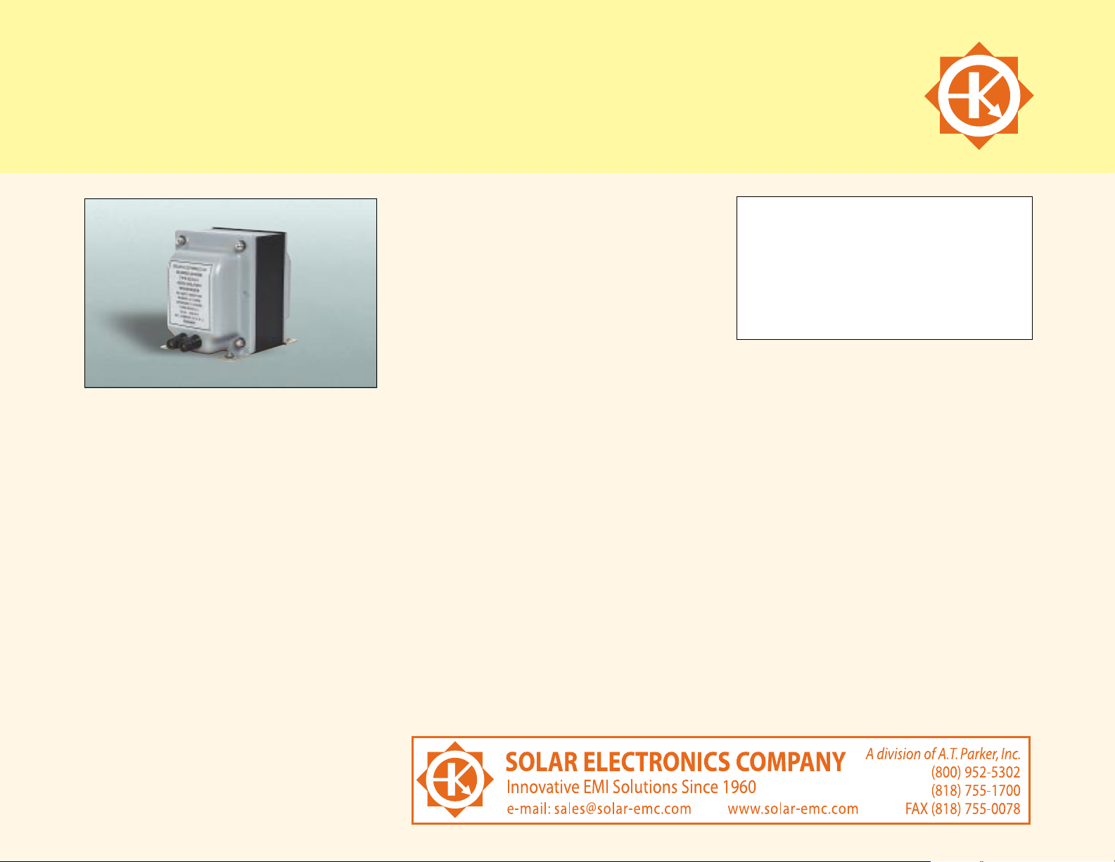
TYPE 6220-1A AUDIO ISOLATION TRANSFORMER
for conducted audio frequency susceptibility testing
APPLICATION
The Type 6220-1A Audio Isolation Transformer
was especially designed for screen room use
in making conducted audio frequency susceptibility tests as required by MIL-STD-461/462 and
other EMI specifications.
The transformer may also be used as a pickup
device to measure low frequency EMI currents at
lower levels than conventional current probes.
In addition, its secondary may be used as an
isolating inductor in the power line during
transient susceptibility tests. (See Application
Note AN622001.)
DESCRIPTION
The transformer is capable of handing up to 200
watts of audio power into its primary over the frequency range 30 Hz to 250 KHz. The turns ratio
provides a two-to-one step down to the special
secondary winding.The secondary will handle up
to fifty amperes of a.c. or d.c. without saturating
the transformer.
Another secondary winding is connected to a
pair of binding posts suitable for connecting to
a.c. voltmeter as directed by the applicable
EMI specifications. This winding serves to isolate
the voltmeter from power ground. Neither the
primary nor the secondary windings are
connected to the end bells of the core. The
transformer may be used as a 4-ohm primary and
1-ohm secondary or 2.4-ohm primary and
0.6-ohm secondary or 2-ohm primary and
0.5-ohm secondary.
FEATURES
Provides a convenient bench model unit
with three-way binding posts on primary
and output voltmeter leads. Standard 0.75"
spacing of binding posts allows use of
standard plugs. High current secondary uses
1
/4-20 threaded studs.
Capable of handling the audio power required
by EMI specifications and up to 50 amperes of
a.c. or d.c. through the secondary in series with
the test sample.
May be used as a pickup device or an isolating
inductor in other tests.
Suitable for fastening to the bench top in
permanent test setups.
SPECIFICATIONS
Primary: Less than 5 ohms.
Secondary: One-fourth the primary impedance.
Frequency Response: 30 Hz to 250 KHz.
Audio Power: 200 watts.
Dielectric Test: 600 volts d.c.primary to
secondaries and each winding to end bells.
Secondary Saturation: 50 amperes a.c. or d.c.
maximum.
Turns Ratio: Two-to-one step down.
Secondary Inductance: Approximately 1.0 mH
(unloaded).
Weight: 18 pounds.
Size: 4.5" wide, 5.25 " high,6.25" deep plus
terminals. (114 mm x 133 mm x 159 mm.)
ADDITIONAL MODELS
Type 6220-2 100 amperes high current
transformer.
Type 6220-4 50 amperes 4 KV transient
voltage HV transformer.
Type 9707-1 10 amperes low current
transformer.
57
Page 2
TYPE 6220-1A AUDIO ISOLATION TRANSFORMER
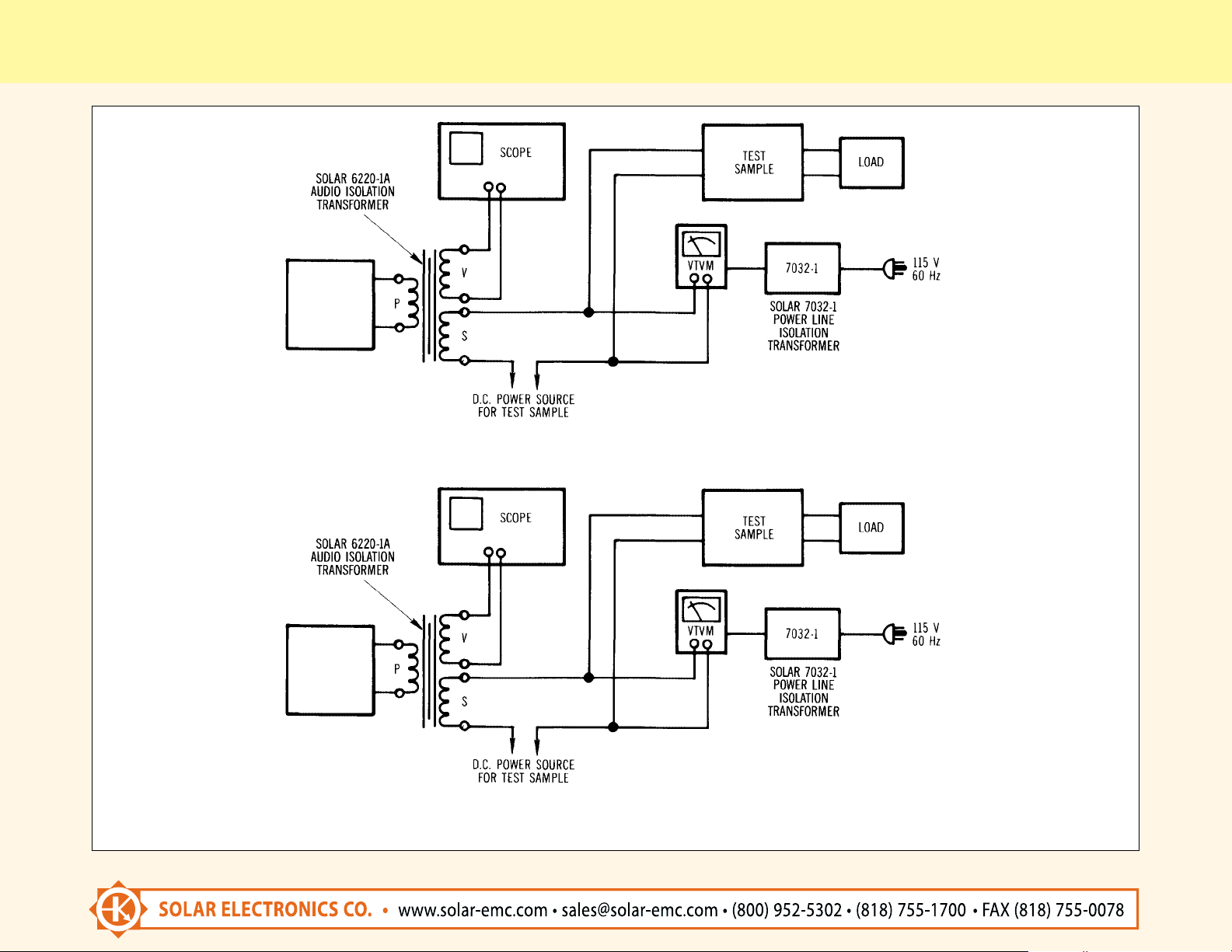
AUDIO SUSCEPTIBILITY TEST SETUP FOR D.C. LINES
TEST SETUP FOR MEASURING LOW FREQUENCY, LOW AMPLITUDE EMI CURRENT
See Application Note 622001
SOLAR
8850-1 or 6550-1
POWER
SWEEP
GENERATOR
SOLAR
8850-1 or 6550-1
POWER
SWEEP
GENERATOR
58
Page 3

APPLICATION NOTE AN622001
USING TYPE 6220-1A TRANSFORMER FOR THE MEASUREMENT OF LOW FREQUENCY EMI CURRENTS
INTRODUCTION
“There is more than one way to skin a cat” your
great grandfather and my father used to say. The
evolution of methods of measuring conducted
interference illustrates this homely expression in a
distorted kind of way.
To start with, a clever and versatile propulsion
engineer named Alan Watton at Wright Field early
in WWII created an artificial line impedance which
represented what he had measured on
the d.c.buss in a twin-engined aircraft. Probably a
DC-3, but memory is dim on this point. Watton’s
work was sponsored by a committee headed by
Leonard W. Thomas (then of Buships) with active
participation by Dr. Ralph Showers of University
of Pennsylvania and others.
So the Line Impedance Stabilization Network
(LISN) was born. It was a pretty good simulation
of that particular aircraft and the electrical
systems it included. But then someone arbitrarily
decided to use this artificial impedance to
represent any power line.
radiation, particularly at the lower frequencies,
since the coupling between power leads at low
frequencies is inductive, not capacitive.
As it turned out, Stoddart was successful in
developing a current probe based on Alan
Watton’s suggestions regarding the torodial
transformer approach which is still the primary
basis used today. However, the development of
the voltage measurement probe suffered for lack
of sensitivity.Watton’s hope had been to provide
a high impedance voltage probe with better
sensitivity than was then available for measurement receivers designed for rod antennas and
50 ohm inputs. Since this effort failed and
Watton’s funds (and probably his interest in the
subject) faded out of the picture, the program
came to a halt.
This meant that the RFI/EMI engineer could either
measure EMI voltage across an artificial impedance which varied with frequency, or he could
measure EMI current flowing through a circuit of
unknown r.f. impedance. Either way, the whole
story is not known. In spite of the unknown
impedance, the military specifications began
picking up the idea of measuring EMI current
instead of voltage.The test setup was simpler and
the current probe was not as limited as the LISN
in its ability to cope with large power line
currents. And the current probe measurement
was also a measurement of magnetic field
At any rate, this impedance suddenly began
appearing in specifications which demanded
its use in each ungrounded power line for
determining the conducted EMI (then known as
RFI) voltage generated by any kind of a gadget.
The resulting test data,it was argued, allowed the
government to directly compare measured
RFI/EMI voltages from different test samples and
different test laboratories.No one was concerned
about the fact that filtering devised for suppressing the test sample was based on this artificial
impedance in order to pass the requirements,but
that the same filter might have no relation to
reality when used with the test sample in its
normal power line connection.
Not until 1947, that is. At that time, this same
Alan Watton, a propulsion engineer having no
connection with the RFI/EMI business, decided
to rectify the comedy of errors which had
misapplied his original brainchild. He was in a
position to place a small R and D contract with
Stoddart for the development of two probes;
a current measuring probe and a voltage
measuring probe. Obviously, he felt that one
needed to know at least two parameters for a true
understanding of conducted interference. The
current probe is not only a measure of EMI
current, it is a measure of the magnetic field
radiation from the wire or cable under test. This
is a more meaningful measure of magnetic
59
Page 4

AN622001 (continued)
radiation. The current probe was somewhat
better than the LISN for measurements below
150 KHz and above 25 MHz but, even so, the
technique was not very sensitive at the lower
frequency end of the spectrum.
A young Boeing EMI engineer named Frank
Beauchamp was the first to apply the current
probe to wideband measurements from 30 Hz to
20 KHz. He was smart enough to realize some of
the problems in this range so he incorporated the
sliding current probe factor into the method of
measurement he spelled out in the Minuteman
Specification, GM-07-59-2617A. The test method
required that the probe factor existing at 20 KHz
should be used for obtaining the wideband
answer in terms of “per 20 KHz” bandwidth. This
meant that the specified limit was not a constant
throughout the 20 KHz bandwidth, but was
varying as the inverse of the probe factor. A very
sensible solution at the time. Regrettably, later
specifications did not follow this lead.
When later EMI specifications extended the need
for measurement of EMI currents down to 30 Hz
without taking into account the sloping probe
factor, the problem of probe sensitivity became
critical. Attempts to compensate for the poor
current probe response at low frequencies by
using active element suffer from dynamic range
difficulties and the possibility of overload.
This led to another way of “skinning the cat,”with
the aid of the Audio Isolation Transformer already
available and in use for susceptibility testing.
The technique described in the following
paragraphs indicates how to obtain considerably
greater measurement sensitivity for conducted
narrowband EMI currents and a means for obtaining a flat frequency characteristic without the use
of active elements for broadband or “wideband”
EMI current measurements.
BASIC CONCEPT
The application described herein has grown out
of a suggestion by Sam Shankle of Philco Ford in
Palo Alto. He and his capable crew first tried this
scheme using H-P Wave Analyzers as the associated voltmeter. Our work with the idea has
concentrated on conventional EMI meters with
50 ohm inputs.
Basically, the test method consists of using the
secondary (S) of the Solar Type 6220-1A Audio
Isolation Transformer as the pickup device.
The transformer winding normally used as the
primary (P) is used as an output winding in this
case. The method provides a two-to-one step up
to further enhance the sensitivity.
USE OF THE TYPE 6220-1A
TRANSFORMER IN GENERAL
Since the transformer is connected in series with
each ungrounded power input lead (sequentially)
for performing the audio susceptibility tests,it can
be used for two additional purposes while still in
the circuit. First, the secondary winding can act
as the series inductor suggested for transient
injection tests to prevent the transient from being
short-circuited by the impedance of the power
line. In this application all other windings are left
open. See Figure 1. Secondly, the transformer
can be used for measuring EMI current as
described herein. See Figure 2. At other times, if
it is not needed in the circuit, short cicuiting the
primary winding will effectively reduce the
secondary inductance to a value so low that the
transformer acts as if it isn’t there.
ACHIEVING MAXIMUM SENSITIVITY
FOR CONDUCTED EMI CURRENT
MEASUREMENTS
The basic circuit in Figure 2 provides the most
pickup and transfer of energy over the frequency
range 30 Hz to 150 KHz. Curve #1 of Figure 3
shows the correction factors required to convert
narrowband signals to dB above one microampere. Since the sign of the factor is negative for
most of the range, the sensitivity is considerably
better than that of conventional current probes.
The sensitivity achieved by this technique is
better than .05 microamperes at frequencies
60
Page 5

above 5 KHz when using an EMI meter capable of
measuring 1.0 microvolt into 50 ohms. For EMI
meters such as the NM-7A and the EMC-10E,
the meter sensitivity is a decade better and
it is possible to measure EMI currents of
.005 microamperes at 5 KHz and above.
FLATTENING THE RESPONSE
At a sacrifice of sensitivity, the upper portion of
the frequency vs. correction factor curve can be
flattened to provide a constant correction factor
from about 1 KHz up to 150 KHz.This is depicted
in curve #2 of Figure 3, where a -20 dB correction
is suitable over this part of the frequency range.
The flattening is obtained by loading the primary
with a suitable value or resistance.The resistance
value used in this example is 10 ohms. The
flattening still allows the measurement of a
0.1 microampere signal when using an EMI meter
with 0.1 microvolt sensitivity. An advantage
of this response curve is the sloping correction
at frequencies below 1KHz which acts like a high
pass filter to remove some of the power line
harmonics from wideband measurements.
If you are only interested in frequencies above
150 Hz, a 2 ohm resistor is all that is needed. See
curve #3.
STILL MORE FLATTENING
Like the girdle ads say,you can firmer and flatter,
with a loss in sensitivity , by further reducing the
value of the shunt resistor. This is illustrated
in curve #4 of Figure 3 where a 0.5 ohm shunt
resistor (Solar Type 6920-0.5) is connected
across the transformer primary winding used as
an output winding to the EMI meter.The overall
flatness is achieved at the sacrifice of considerable
sensitivity, but the sensitivity is well under the
requirements of existing specifications and the
correction network utilizes no active elements.
LIMITATIONS OF THE METHOD
When measuring EMI current on d.c. lines, there
are no problems,but on a.c. lines there are limitations.The a.c. voltage drop across the winding (S)
due to power current flowing to the test sample
is the principal problem. This voltage induces
twice as much voltage in the output winding (P)
at the power frequency. Since we prefer to limit
the power dissipation in the 50 ohm input to the
EMI meter so that it will not exceed 0.5 watts,the
induced voltage must be kept below a safe limit.
For 400 Hz lines, the power frequency current
must not exceed 16 amperes to avoid too much
400 Hz power dissipation in the input to the EMI
meter. Also, the resistance ‘R’ used across the
output winding (P) must be at least a 50 watt
rating on 400 Hz lines. This resistor should be
noninductive to avoid errors due to inductive
reactance.
THINGS TO BE WARY OF
The 10 F feed-thru required by present
day specs has appreciable reactance at 30 Hz
( 54 ohms) and acts to reduce the actual EMI
current flowing in the circuit. This means less
trouble in meeting the spec,but when calibrating
the test method described herein, it is wise to
short circuit the capacitor.
In the case where the input circuit to the
EMI meter is reactive, such as the EMC-10E, it is
necessary to use a minimum loss ‘T’ pad at
the input to the meter. The Eaton NM-7A and
NM-12/27A units do not require this pad and
its loss.
DETERMINING THE NARROWBAND
CORRECTION FACTOR
The test setup of Figure 4 describes the simple
method of determining either the transfer
AN622001 (continued)
FIGURE 3 – TYPICAL CORRECTION DATA VS. FREQUENCY
61
dB TO BE ADDED TO EMI
METER READING (IN dB) TO
+20
+10
0
–10
–20
–30
10 100 1K
OBTAIN dB / A.
FREQUENCY HERTZ
CURVE #4
R0.5 OHM
CURVE #3
R2 OHMS
CURVE #2
R10 OHMS
CURVE #1
R=
∞
10K
100K
1M
Page 6

impedance or the correction curve, whichever is
desired. Actually, there is no need to plot the
answer as transfer impedance, since the desired
end product is the correction factor to be applied
to the meter reading to obtain decibels above
one microampere. The correction must be
obtained for each configuration. In other words,
if you want to use the method for maximum
sensitivity, the calibration is performed with just
a 50 ohm load on the primary winding simulating
the EMI meter. If the flattening networks will be
used,then they must be connected to the primary
winding during the calibration and must be
further loaded with 50 ohms to simulate the EMI
meter input.
At each test frequency, the output of the audio
signal generator is adjusted for a level which
delivers the same current to the secondary (S) of
the transformer.This is accomplished by setting a
constant voltage across the 10 ohm resistor. A
convenient level is 0.1 volt across 10 ohms which
is 10,000 microamperes (80 dB/uA).
Adjust the gain of the EMI meter to assure a one
microvolt meter reading for a one microvolt R.F.
input from a standard signal generator. Then
connect the 50 ohm input circuit of the EMI meter
to the primary of the 6220-1A. If the EMC-10E is
used,insert a 10 dB pad in series with the input. If
the calibration is for maximum sensitivity, no
additional loading is necessary. If the calibration
is for the flattened versions discussed above, the
appropriate resistance must be connected across
the primary of the transformer.
At the frequency of the test, set the output of the
signal source to obtain 1.0 volt across the 10 ohm
resistor. Carefully tune the EMI meter to the test
frequency and note the meter reading on the dB
scale. The difference between the meter reading
in dB and 80 dB represents the correction neces-
sary to convert the meter reading to dB above
one microampere for narrowband measurements.
In most cases, the correction will have a negative
sign. For example, at 100 Hz the EMI meter
may read 88 dB above one microvolt. Since the
reference is 80 dB above one microampere, the
correction is -8 dB to added algebraically to
the meter reading to obtain the correct reading
in dB above one microampere.
If the 10 dB pad has been used, this loss must be
accounted for in deriving the correction. If the
pad will be used in the actual test setups, its loss
becomes part of the correction factor.In this case,
the meter reading obtained in the foregoing
example would be 78 dB above one microvolt
and the correction factor would be +2 dB for
narrowband measurements.
Repeating this procedure at a number of test
frequencies will produce enough data to plot
a smooth curve for use when actual tests are
being conducted.
DERIVING THE BROADBAND
CORRECTION FACTOR
When making broadband measurements as
required by MIL-STD-461A in terms of “dB above
one microampere per megahertz,” use the
average of the narrowband factors over the range
30 Hz to 14 KHz and add a bandwidth correction
factor of 37 dB.
In the case of Method CE01 of MIL-STD-461A, use
the 20 KHz wideband mode of the EMI meter,
determine the average of the narrowband factors
over the range 30 Hz to 20 KHz and use this figure
as the bandwidth correction factor.
When using high pass filters at the input to the
EMI meter to eliminate the first few harmonics
of the power line frequency as allowed by
MIL-STD-461A, the range covered will depend
upon the cutoff frequency of the filter. For
example, on 60 Hz power lines and using Solar
Type 7205-0.35 High Pass Filter between
the 6220-1A Transformer and the EMI meter,
obtain the average narrowband correction
between 350 Hz and 14 KHz and add the bandwidth correction factor of 37 dB. On 400 Hz lines
when using the Solar Type 7205-2.4 High Pass
Filter between the transformer and the EMI
meter,determine the average of the narrowband
factors in the range of 2.4 KHz and 14 KHz and
add the bandwidth correction factor of 38.5 dB.
SUMMARY
Some of the material given in this Application
Note is terse and given without much explanation. If your are confused by this simplification,
just call us.Incidentally,the Signal Corps liked this
method so well that they included it in Notice #3
to MIL-STD-462 date 9 Feb 71.
AN622001 (continued)
FIGURE 4 – TEST SETUP
FOR DETERMINING CORRECTION FACTOR
62
 Loading...