

Page 1
TM
Interface Manual
Continuous Level Controls
7100
™
Leak Detect Stik
Magnetostrictive LeveL systeM
ABSOLUTE PROCESS CONTROL
KNOW WHERE YOU ARE... REGARDLESS
Page 2

.
Page 3

Contents
Chapter 1: Description of Probe .............................2
1.1 Data Protocol ....................................................2
1.2 Frame Protocol ...................................................3
1.3 Installation and Dimension Drawings ..................................5
Chapter 2: Interfacing to Probe..............................8
2.1 Interface Hardware ...............................................10
Chapter 3: Getting the Data................................ 12
3.1 Synchronizing with a Watchdog Timer ................................12
3.2 System Hardware Setup...........................................12
3.3 System Software Setup ...........................................13
Chapter 4: Processing the Data ............................14
4.1 Front End Algorithm ..............................................14
Chapter 5: Computing the Temperature ......................15
5.1 Improving Measurement Accuracy ...................................15
EC Certicate of Conformity ...........................................18
AMETEK has checked the accuracy of this manual at the time it was printed. Any comments you
may have for the improvement of this manual are welcomed.
AMETEK reserves the right to revise and redistribute the entire contents or selected pages of this
manual. All rights to the contents of this manual are reserved by AMETEK.
The information in this document is subject to change without notice. No part of this document may
be reproduced or transmitted in any form or by any means, for any purpose, without the express
written permission of AMETEK.
Page 4

Chapter 1: Description of Probe
The 7100 liquid level probe uses a proprietary data transmission technique providing a compact information
format for level and temperature data, and a signal pattern which is very easily recognizable at the console.
1.1: Data Protocol
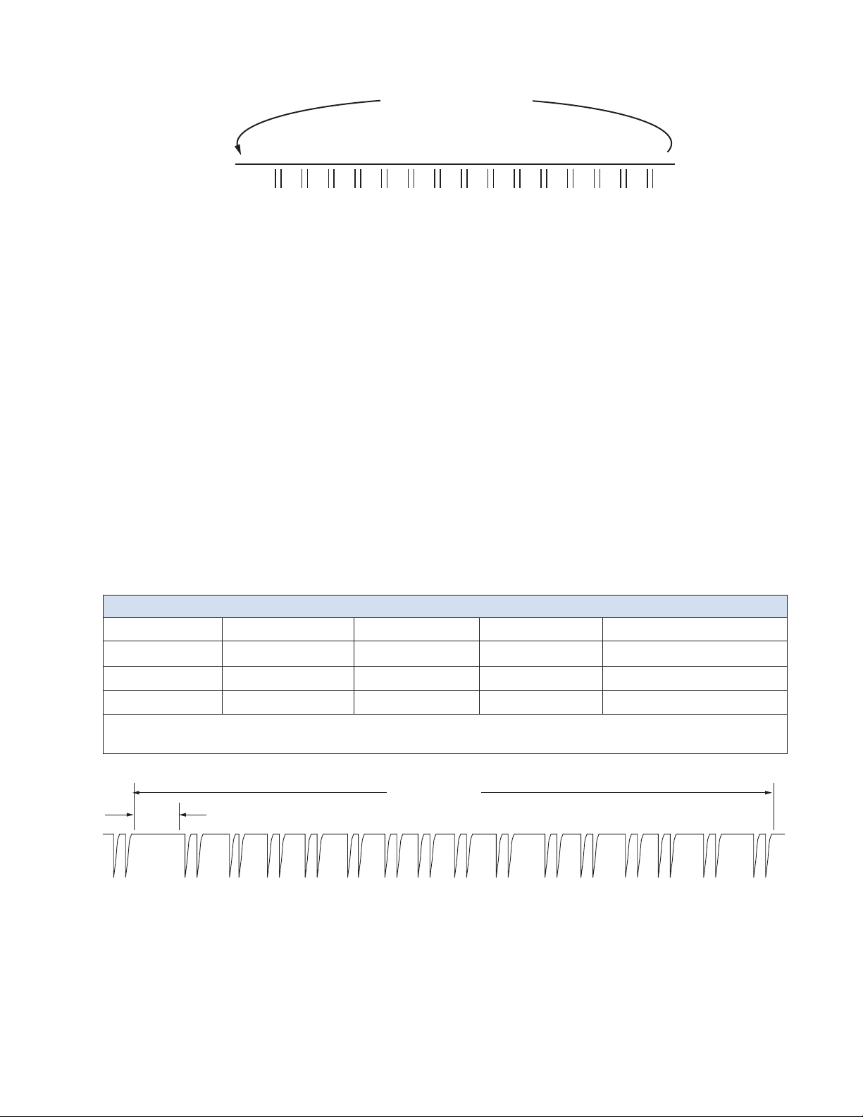
Transmission consists of a sequence of similarly formatted frames of data, each frame in turn, consisting
of 15 pulse pairs and a pause period. The pause period, as well as the 15 pulse pairs, each occupy 1 of 16
equal time slots of approximately 4.5 milliseconds¹.
Time slot #1 is the pause period and carries no signals. This pause is used by the console to synchronize
with the signal sequence. After this pause is found, no further recognition operations are necessary; the
console can simply follow the sequence described below. Each of the remaining 15 time slots carries two
pulses. The time interval between the pulses in each pair is equal to a value of the parameter assigned to the
corresponding time slot. (See Figure 1)
Even numbered pulse pairs #2, 4, 6, 8, 10, 12, 14, & 16 carry temperature related data.
The time interval between the pulses in time slot #3 is proportional to the water level (the lower oat position).
The six remaining odd numbered pulse pairs #5, 7, 9, 11, 13, & 15 carry signals related to the product signal.
Thus, information on the product level collected during one frame increases the initial resolution (determined
by the frequency of the clock advancing the high speed counters in the console) by a factor of about 2.5
(square root of 6). See footnote².
The entire message, including time slot #1 through
#16, is referred to as a Frame of data throughout
this document.
NOTE: The first pulse pair in a frame is in
time slot #2 and is hence referred to
as pulse pair #2. As stated above, the
eight even pulse pairs #2, 4, 6, 8, 10,
12, 14, & 16 carry temperature data. #2
through #10 correspond to the lowest to
the highest temperature sensors in the
probe rod, respectively. #12 corresponds
to the temperature sensor in the head
electronics. #14 and #16 are references.
The ve sensors are spaced apart equally
in the probe rod. (See Chapter 5 for more
information on computing the temperature).
¹ For probes over 18 feet in length, the frame duration should
be doubled. This is due to the longer wire propagation time.
² Since the magnetostrictive wire velocity is about 9
microseconds per inch, a 110 MHz. clock would provide a
single level readout resolution of 0.001”. Since the 7100 probe
utilizes the patented resolution-doubling reection method,
the resolution would be 0.0005”. If a more practical 40 MHz.
clock is used, the resolution is 0.001375”.
Input Voltage 16 to 31 VDC
Sensor Length
Enclosure Rating Material 316 SS or PVDF, IP 68
Typical Level Resolution
(Controller Dependent)
Linearity
Repeatability
Temperature Measurement Up to 5 along the sensor span
Temperature Accuracy, Absolute +/- 2°F
Typical Temperature Resolution
(Controller Dependent)
Temperature Sensing Range - 40°F to +158°F or -40°C to 70°C
Operating Temperature Range - 40°F to +158°F or -40°C to 70°C
Sensor Output Pulse Position Modulated
Distance to Monitor Over 1000’ using twisted pair wire
Floats (not included) Specs based on 4” standard oats
Approvals
Specications
Stainless Steel up to 24’
PVDF up to 70’
0.010” Inventory Mode
0.001” Leak Detection Mode
+/- 0.01% of Full Scale
+/- 0.010”, whichever is greater
+/- 0.001% of Full Scale
+/- 0.00025”, whichever is greater
+/- 0.01°F
NORTH AMERICA
CLASS I,II,III, DIVISION 1,
GROUPS D,E,F,G: T4 (7100 K&V)
GROUPS C,D,E,F,G,: T4 (7100 M&R)
Exia SECURITE INTRINSEQUE
EUROPEAN UNION IEC
CE 0575
II 1 G
Ex ia IIA T4 Ga (7100 K&V)
Ex ia IIB T4 Ga (7100 M&R)
IECEx UL 11.0041X
DEMKO 09 ATEX 0902049X
LISTED
14X7
Specications are subject to change without notice. Patented.
2
Page 5
Return to Start of Frame
16 Time Slots
#1 #2 #3 #4 #5 #6 #7 #8 #9 #10 #11 #12 #13 #14 #15 #16
Pause
Water
Temp #1
Product
Temp #2
Product
Temp #3
Product
Temp #4
Product
Temp #5
Circuit Temp
Product
Low Ref
Product
High Ref
Figure 1: One frame of Data
1.2: Frame Protocol
All 7100 probes transmit data in the same general format. In this format, information is conveyed during a
discrete period of time called a frame. The duration of a frame varies depending on the probe type. Table 1
species the frame periods for various probe types.
7100 series probe data consists of a series of pulses that are transmitted along the wire pair that provides
power to the probe. Pulses are grouped in pairs called readings. Position and temperature information can be
determined by measuring the period between the two pulses that comprise a reading.
A frame consists of a sync. period followed by 15 readings. The sync. period is a period of time during which
no pulses occur. An external device that is attempting to synchronize with the probe data should start looking
for the rst pulse in reading 1 after detecting a period greater than sync. period during which no pulses occur.
Table 1 lists the recommended sync period for various probe types.
Table 1 - 7100 Probe parameters by probe type
Probe Type Overall Length Frame Period Sync Period Reference Magnet
Types 1, 4
Types 2, 5
Types 3, 6
0 < L ≤ 18
18 < L ≤ 24
24 < L
NOTE: Probe types 1, 2, and 3 are 5 thermistor probes (R5 designation in part number). Probe types 4, 5,
and 6 are 1 thermistor probes (R1 designation in part number).
72 ms 7 ms No
144 ms 16.6 ms No
144 ms 16.6 ms Yes
Frame Period
Sync
Period
Reading 15
Reading 1
Reading 2
Reading 3
Reading 4
Reading 5
Reading 6
Reading 7
Reading 8
Reading 9
Reading 10
Reading 13
Reading 11
Reading 12
Reading 14
Figure 2: Data Frame Relationship Between the Data Pulses, Sync and Frame Periods
Reading 15
3
Page 6

The type of information contained in each reading varies depending on the probe type. Table 2 species the data
pattern for various probe types.
Table 2 - Reading Data Type Specication by Probe Type
Types 1, 2, 3 Types 4, 5, 6
Reading 1 Temp 1 Temp 1
Reading 2 Product or Water* Product or Water*
Reading 3 Low Ref Temp Temp 2
Reading 4 Product Product
Reading 5 High Ref Temp Temp 3
Reading 6 Product Product
Reading 7 Low Ref Temp Temp 4
Reading 8 Product Product
Reading 9 High Ref Temp Temp 5
Reading 10 Product Product
Reading 11 Circuit Temp Circuit Temp
Reading 12 Product Product
Reading 13 Low Ref Temp Low Ref Temp
Reading 14 Product Product
Reading 15 High Ref Temp High Ref Temp
* For single oat probes, this frame contains product data.
For dual oat probes, this frame contains water data.
When calculating Water or Product positions, one must consider whether or not the probe uses a reference
magnet. For probes that use a reference magnet (type 3 and type 6), position can be calculated using the
following formula:
Position = Measured Period/Wire Speed
Where:
Measured Period = the time between pulses in a reading (ms)
Wire Speed = (ms / inch)
Position = distance from internal reference
For probes that do not use a reference magnet (types 1, 2, 4, and 5), position can be calculated using the
following formula:
Position = Measured Period/Wire Speed*2
4
Page 7
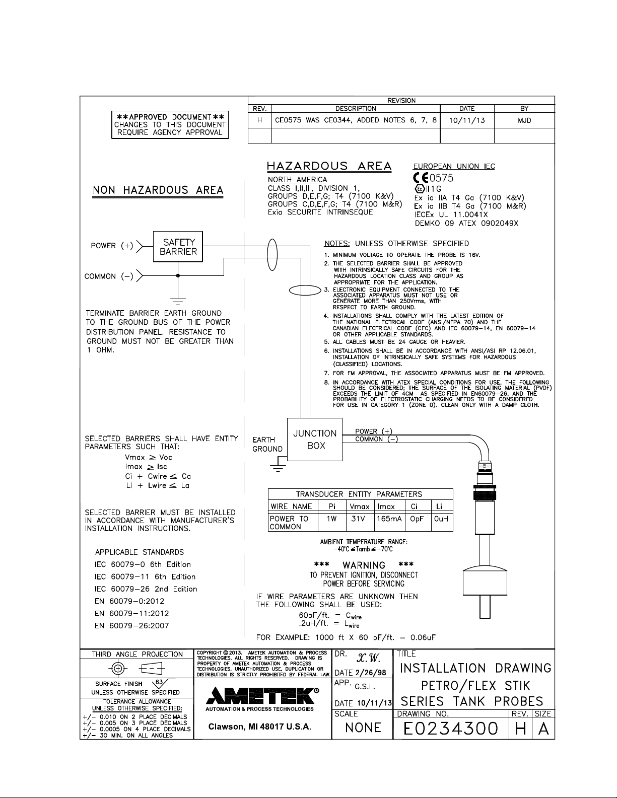
1.3: Installation and Dimension Drawings
7100 Flex Stik Installation Drawing
5
Page 8

7100 Dimension Drawing, Page 1
6
Page 9

7100 Dimension Drawing, Page 2
7
Page 10

Chapter 2: Interfacing to Probe
0 VDC
The pulse signals coming from the probe are superimposed onto the nominal 24 VDC power supply
connections. As shown in Figure 3, the pulses are negative-going and are large in amplitude, nominally 20
volts peak. The peak is negative going and only a few microseconds in duration. The leading edge is the
proper edge to use for timing purposes. The large signal amplitude offers high noise immunity.
Pulse Pair
24 VDC
24 Volt Power
Supply Level
Figure 3: Pulse Signals
A simple approach to getting 5 volt logic levels from the input signal is to simply set a comparator level as
shown in Figure 6. The comparator output can then be used to create a gate signal for a counter circuit. The
circuit example in Section 2.1 (page10) has a variation of this concept using a 5:1 pulse transformer to eliminate the reference to 24 VDC and make the comparison relative to circuit common (with inverted polarity).
Probe power supply impedance will have an effect on pulse amplitude. Wire lengths will vary the pulse amplitude. Wire has an associated inductance, resistance and capacitance which will change the amplitude of the
coupled pulse. Users may wish to load their circuit to minimize wire effects.
The chart below gives relative times by which a user can distinguish timing for various probe lengths.
Length Float Position Tstart Tstop Dt=Position
12" 1" 160msec 180msec 20msec
12" 12" 50msec 290msec 240msec
30" 1" 340msec 360msec 20msec
30" 30" 50msec 650msec 600msec
100" 1" 1040msec 1060msec 20msec
100" 100" 50msec 2050msec 2000msec
200" 1" 2040msec 2060msec 20msec
200" 200" 50msec 4050msec 4000msec
8
Page 11

4.5mS
Reset Reset Watchdog Watchdog
t
s-s
4.5mS
Figure 4: Start Pulse
NOTE 1: t
= time from 1st start pulse in one frame to next start pulse in the next frame.
s-s
NOTE 2: Start pulse can start anywhere in the 4.5 ms frame. The stop pulse will follow at the correct time.
The t
is not consistent. The user does not have the 4.5 ms frame as a reference. The user must
s-s
use the watchdog timeout during the pause frame to “sync up”. The watchdog timer should be reset
on both the start and stop pulse.
4.5mS
#15 #16 #1 #2 #3
Product
High Ref
9mS
Pause
4.5mS
Water
Temp #1
Figure 5: Pause Period Timing
NOTE: Although the timebase is generated with a crystal oscillator, the times shown are NOT exact times.
Also, the initial pulse within a window of the frame does not start at the beginning of the window. See
Section 3.1: Synchronizing with a Watchdog Timer and footnote 3 for more information.
9
Page 12

2.1: Interface Hardware
A typical console has the following sub-systems:
1. Probe Mulitplexer
2. Intrinsic Safety Barrier
3. Pulse Discriminator
4. Gate Circuit
5. High Speed Counter
Use leading edges
of comparator
output to start and
stop counters.
Comparator
Threshold
Comparator
Output
Gate Signal for
Counters
Figure 6: Start and Stop Counters
Figure 7 shows typical means of achieving each of these sub-systems. The multiplexing is achieved with the
use of a PNP-style bipolar driver IC. where only one output is turned on at a given time. The output that is
turned on serves two functions; it couples power to the corresponding probe, and it conducts the probes output pulses back to the pulse discriminator.
The intrinsic safety barrier is achieved where the dotted line is shown.
A Stahl Intrinspak 9001/01-280-110-101 could be used as an "off-the-shelf" barrier when installed in accordance per Stahl manual 9001/60/301 and local safety standards. Safety barrier entity parameters must meet
the requirements as called out in installation drawing E0234300.
The pulse discriminator is comprised of a 5:1 pulse transformer that is capacitively coupled to the intrinsically safe power supply (where the probe pulses are found) and used to invert the pulses, amplify them, and
remove the 24 VDC. offset. Finally, a comparator is used to generate the nal output used to drive the gate
circuit. The comparison is done with a nominal threshold voltage of approximately 1 VDC.
The gate and counter circuits are shown only in block diagram form. The clock feeding the counters should be
selected to yield the resolution required (see footnote 2, page 2). The gate circuit should enable the counters
upon the rst pulse in a pulse pair and disable the counters on the second after which the counter values are
taken. The gate signal is also used to alert the resident computer that it is time to take the data.
For clock frequencies above 35Mhz., it is recommended that all analog comparators and digital gating circuit
components be relatively high speed. (If FAST or ACT logic is used for the counters, then also use it for the
gating circuits.)
10
Page 13

5 Volt Logic
Probe Select Lines
49.9K
Metal Film
2981 or Equivalent
(PNP Driver I.C.)
VCC
8 Probe
Connections
GND
(only one line is
active at a time.)
5:1 Pulse
Transformer
+1 VDC
Reference
s
GNDVCC
0.1 uF.
Return signals are coupled through the VCC Pin and the
150 Ohm barrier resistor and coupling capacitor to the
step-up pulse transformer. The inductor passes the 24
Volts without shorting the return pulse.
Always use the
leading edge
150
1 mH.
+24 VDC
Intrinsic Safety Barrier
High Speed Clock
(20-110 mH)
-
Comparator
+
Counter
Gating Circuit
Figure 7: Typical Console Circuitry
High Speed
Counters
Latch
Microcomputer
11
Page 14

Chapter 3: Getting the Data
The method that data is communicated between the probe and the console is described in Section 1.1: Data
Protocol. The user should understand the data protocol scheme before attempting to process the data.
3.1: Synchronizing with a Watchdog Timer
Referring to Figures 1 and 5, note that there is only one pause period per frame and therefore, only one
time during the sequence when no pulses will be received for approximately 9 milliseconds. A hardware or
software watchdog timer may be implemented to time-out after 7 milliseconds (for probes > 18’, this time
should be 14 milliseconds) which will occur only during frame #1, the pause frame. The next 15 pulse pairs
may then be recorded in the sequence shown in Figure 1.
NOTE: The times depicted in Figure 5 are not exact times³. A watchdog timer setting of 7 milliseconds should
generally be used.
3.2: System Hardware Setup
Before discussing signal processing, a brief review of the console hardware is in order. Refer to Section 2 as
required.
Based on a 16 foot maximum probe length, the number of bits required for the probe counter circuit is the
duration of the low reference temperature pulse pair. With a 3 ms low reference pulse duration and a 100
MHz clock frequency, the number of bits can be calculated. Dividing the low reference pulse pair duration by
the period of the clock yields 300,000 counts. Converting this number to hexadecimal will show the number of
required bits. In this case, 19.
³ Although the time between adjacent frames is generated with an internal crystal oscillator, the actual pulse pair for a temperature
frame is delayed a few hundred microseconds nominally. This is independent of any temperature data. The product and water oat
pulse pairs may be delayed as much as 2 milliseconds. This delay is affected by the corresponding oat position. The longest delay is
experienced with a long probe with the oat near the bottom.
12
Page 15

3.3: System Software Setup
Although one frame of data is sufcient to obtain valid product, water, and temperature readings, averaging
multiple frames is generally much more appropriate. This is because all elements in the system are subject
to slight uncertainties and/or the effects of electrical noise or mechanical vibration. This includes the
magnetostrictive wire in the probe, the probe electronics, the transmission wire between the probe and the
console, and the console electronics.
The number of frames of data required for a good probe reading is application dependent. Since the number
of frames of data taken is directly proportional to the console update time, the user should review the system
criterion before implementing a design. For the sake of discussion, 16 frames of data will be taken. The
following table shows the particulars of a console taking in 16 frames of data.
Parameter Result Notes
Frames Read 16 16 Frames as dened
Pulse Pairs Read 240 16 Frames x 15 Pulse Pairs/Frame
Product Pulse Pairs 96 16 Frames x 6 Pulse Pairs/Frame
Water Pulse Pairs 16 16 Frames x 1 Pulse Pairs/Frame
Temp. Pulse Pairs 128 16 Frames x 8 Pulse Pairs/Frame
Pause Pulse Pairs 0 NO PULSE DURING PAUSE
Console Update Time 1.17 Seconds See Below
Required Memory 720 Bytes See Below
The update time is calculated as:
t
update
NOTE: This update time does not include the time required to become synchronized. Up to one additional
frame is necessary to synchronize making the total 1.24 seconds.
The required memory is calculated as:
Memory Bytes
The user will want to congure the system based on individual requirements for update time and memory
space. Readings are more precise when more frames are read but more time and memory are required.
= 16 Frames x
= 16 Frames x
16 Time Slots
{
1 Frame
{
}x{
15 Pulse Pairs
1 Frame
4.57 Milliseconds
1 Time Slot
}x{
3 Bytes
1 Pulse Pair
= 1170 Ms.
}
= 720 Bytes
}
13
Page 16

Chapter 4: Processing the Data
Data acquisition was discussed in Section 3 to the degree that memory locations are lled with an array of
data from a selected number of frames. It is now appropriate to test for data integrity, average and/or lter the
data, and then convert from binary counter values to scaled, meaningful numbers.
4.1: Front End Algorithm
A technique for eliminating any possible erroneous data is to discard some of the highest and lowest count
values. Lets assume that there is some uncontrolled source of harsh electrical noise causing erroneous data
to be received once approximately every 100 to 1000 frames. The table below shows appropriate numbers of
High and Low discard values to ensure that no erroneous data is used.
Parameter Highs
Discarded
Product 12 12 72 of 96
Water 2 2 12 of 16
Temp #1 2 2 12 of 16
Temp #2 2 2 12 of 16
Temp #3 2 2 12 of 16
Temp #4 2 2 12 of 16
Temp #5 2 2 12 of 16
Circuit Temp 2 2 12 of 16
LO Reference Temp. 2 2 12 of 16
HI Reference Temp. 2 2 12 of 16
After discarding the Highs and Lows, the remaining data is averaged and the results are referred to as one
Probe Reading. These discard numbers are only guidelines. They may be changed to accommodate more or
less frequently encountered noise problems, depending upon the installation environment.
One probe reading contains ten values, one for product level, one for water level, and eight for temperature.
Lows
Discarded
Probe Reading is the Average of
14
Page 17

Chapter 5: Computing the Temperature
A probe reading contains 15 values for product, water and temperature. The product and water values are
each useful by themselves (a single product or water value may be converted with linear math to represent
the oat position).
Unlike the product and water values, the temperature values are always accompanied by two reference
values. A single temperature sensor value is of no use without its associated reference temperature
values. The use of reference values eliminates the effects of circuit drift and produces exceptionally good
repeatability.
The 7100 Liquid Level Probe uses thermistors as the temperature sensing elements. All thermistors exhibit
known, well dened non-linearity. In our application, the non-linearity of the temperature data is in the range of
a few percent. (See Section 5.1: Improving Measurement Accuracy)
As shown in Section 5.1: Improving Measurement Accuracy, the rst step in computing the temperature of
a given sensor is to use a linear equation to interpolate between the reference temperatures. The above
mentioned non-linearity will then be present in the result.
5.1: Improving Measurement Accuracy
The temperature measurement circuitry of the 7100 probe generates temperature pulse pairs with the time
interval directly proportional to the resistance of a parallel connected thermistor (or reference temperature
resistor) and a xed 37.4 K resistor. The 37.4 K parallel resistor serves to keep the time range of the
temperature pulses within reasonable limits over the probe’s temperature range.
Variations in parameters of thermistors, time dening capacitors, and other parts of the probe introduce
additional error to the temperature measurement. To reduce this error the 7100 probe transmits signals for
two reference temperatures: +5 °C (low reference), and +50 °C (high reference). The following sequence of
calculations compensates for errors using the reference signals, and takes into account the thermistor plus
37.4 K resistor non-linearity.
Step 1 - Get reliable time counts for each temperature read, including the temperature references.
Example:
1) Take 16 reads of a temperature.
2) Discard 2 highest and 2 lowest readings.
3) Take average value of the 12 remaining readings.
Step 2 - Calculate linear approximation of temperature (T
T
= [(R - L) * (H
LIN
REF
- L
) / (H - L)] + L
REF
REF
) using the following formula:
LIN
Where:
R = counts for thermistor,
L = counts for low reference,
H = counts for high reference,
L
H
= low reference = 5 °C,
REF
= high reference = 50 °C.
REF
T
is a normalized value for temperature that compensates for errors caused by variations of the probe
LIN
parts’ parameters. This is not actual temperature yet. It does not take into account non-linearity of the
thermistor-parallel resistor combination.
15
Page 18

Step 3 - Using the attached table, nd the linear temperature interval (T
temperature interval (T1, T2) for T
LIN
.
Example.
LIN1
, T
) and then the actual
LIN2
T
T
T
= 15.763 °C,
LIN
= 15.178 °C,
LIN1
= 16.321 °C,
LIN2
T1 = 14 °C,
T2 = 15 °C.
Step 4 - Calculate accurate table interpolated temperature T, using linear interpolation within intervals (T
T
) and (T1, T2).
LIN2
T = ((T
LIN2
- T
LIN1
) * T2 - (T
LIN2
- T
) * (T2 - T1)) / (T
LIN
LIN2
- T
LIN1
)
Example:
T
T
T
= 15.763 °C,
LIN
= 15.178 °C,
LIN1
= 16.321 °C,
LIN2
T1 = 14 °C,
T2 = 15 °C,
T = 14.512 °C
LIN1
,
16
Page 19

Temperature Calculation Table
Actual
Temp
°C
-40 -25.141 0 -0.325 40 42.332 80 63.706 120 70.136
-39 -24.884 1 0.709 41 43.185 81 63.984 121 70.215
-38 -24.613 2 1.759 42 44.016 82 64.250 122 70.296
-37 -24.327 3 2.828 43 44.824 83 64.511 123 70.370
-36 -24.030 4 3.904 44 45.618 84 64.766 124 70.444
-35 -23.714 5 5.000 45 46.386 85 65.009 125 70.524
-34 -23.386 6 6.102 46 47.155 86 65.246 126 70.586
-33 -23.038 7 7.214 47 47.893 87 65.477 127 70.653
-32 -22.678 8 8.331 48 48.618 88 65.696 128 70.719
-31 -22.297 9 9.461 49 49.317 89 65.913 129 70.782
-30 -21.900 10 10.598 50 50.000 90 66.121 130 70.844
-29 -21.488 11 11.738 51 50.665 91 66.323 131 70.905
-28 -21.055 12 12.875 52 51.320 92 66.519 132 70.963
-27 -20.601 13 14.032 53 51.955 93 66.711 133 71.020
-26 -20.133 14 15.178 54 52.575 94 66.894 134 71.075
-25 -19.641 15 16.321 55 53.177 95 67.072 135 71.128
-24 -19.126 16 17.472 56 53.761 96 67.245 136 71.180
-23 -18.598 17 18.629 57 54.331 97 67.413 137 71.231
-22 -18.042 18 19.770 58 54.882 98 67.576 138 71.281
-21 -17.466 19 20.907 59 55.423 99 67.734 139 71.328
-20 -16.871 20 21.974 60 55.942 100 67.886 140 71.375
-19 -16.249 21 23.173 61 56.451 101 68.034 141 71.420
-18 -15.611 22 24.295 62 56.943 102 68.180 142 71.464
-17 -14.945 23 25.419 63 57.423 103 68.319 143 71.507
-16 -14.258 24 26.518 64 57.890 104 68.453 144 71.548
-15 -13.554 25 27.611 65 58.344 105 68.583 145 71.589
-14 -12.823 26 28.695 66 58.779 106 68.710 146 71.629
-13 -12.068 27 29.767 67 59.205 107 68.833 147 71.667
-12 -11.291 28 30.822 68 59.618 108 68.954 148 71.703
-11 -10.497 29 31.866 69 60.022 109 69.070 149 71.740
-10 -9.671 30 32.899 70 60.410 110 69.181 150 71.775
-9 -8.832 31 33.914 71 60.783 111 69.290
-8 -7.968 32 34.920 72 61.153 112 69.396
-7 -7.078 33 35.903 73 61.506 113 69.498
-6 -6.178 34 36.868 74 61.849 114 69.597
-5 -5.252 35 37.830 75 62.182 115 69.694
-4 -4.297 36 38.759 76 62.510 116 69.789
-3 -3.332 37 39.677 77 62.821 117 69.879
-2 -2.347 38 40.582 78 63.127 118 69.968
-1 -1.345 39 41.472 79 63.422 119 70.053
Linear
Temp
°C
Actual
Temp
°C
Linear
Temp
°C
Actual
Temp
°C
Linear
Temp
°C
Actual
Temp
°C
Linear
Temp
°C
Actual
Temp
°C
Linear
Temp
°C
NOTE: Consult the factory if calculations within a larger temperature range is required.
17
Page 20

EC Declaration of Conformity
Manufacturer:
6380 Brockway Road, Peck, MI 48466 USA
Identification of Equipment:
7100 Stik Series Liquid Level Transducer
Description of Device:
The device is a permanently mounted liquid level probe. It determines the level of a liquid based on
signal reflections, caused by magnetic floats, in a wire running the length of the probe. These signals are
amplified and processed, then relayed via a signal imposed on the input wires to the probe. The probe
body and tube may be constructed of stainless steel or of a flexible PVDF polymer. These devices also
take liquid level temperature measurements using thermistors located inside the probe tube.
EC type certificate: DEMKO (0539) 09ATEX0902049X
Lyskaer 8, P.O. Box 514, 2730 Herlev, Denmark
Conformity Specifications: models 7100 M/R:
models 7100 K/V: II 1 G Ex ia IIA T4 Ga Ta: -40ºC to +70ºC
Council Directives:
Directive 94/9/EC, ATEX
Directive 89/336/EEC, EMC
Harmonized Standards:
EN60079-0:2012
EN60079-11:2012
EN60079-26:2007
EN61010-1:2010
Electrical apparatus for explosive gas atmospheres - Part 0:
General requirements
Electrical apparatus for explosive gas atmospheres - Part 11: Intrinsic
safety "i"
Explosive atmospheres – Part 26:
Construction, test and marking of group II category I G electrical
apparatus
Safety Requirements for Electrical Equipment for Measurement,
Control, and laboratory Use
AMETEK Automation & Process Technologies
II 1 G Ex ia IIB T4 Ga Ta: -40ºC to +70ºC
Other Standards:
Limits and methods of measurement of radio characteristics of
EN55011:1998
EN50082-1:1992
IEC 801-2:1984 ESD Susceptibility
IEC 801-3:1984 Radiated Susceptibility, Electromagnetic Field
IEC 801-4:1988 Conducted Susceptibility, Burst Interference Transients
Signed:
Name: Glenn S. Loding Dated: 10/25/13
Position: Engineering Manager Company: AMETEK Automation & Process Technologies
18
industrial, scientific and medical (ISM) Radio Frequency equipment,
Class B, Group 1
Electromagnetic compatibility Generic immunity standard Part 1.
Residential, commercial and light industry
Page 21

Page 22

Other Products
MADE IN AMERICA
© Copyright 2013. All Rights Reserved. Made in the USA.
®
1080 North Crooks Road, Clawson, MI 48017
Phone: 248-435-0700 Toll Free: 800-635-0289
Email: apt.orders@ametek.com Web: www.ametekapt.com
7100IFC.M7R
10/13.Z61
 Loading...