AGO LF-HF User Guide

AGO Field Manual

Dartmouth College LF-HF Receiver

May 10, 1996

1 I

ntroduction

Many studies of radiowave propagation have been performed in the LF/MF/HF radio
bands, but relatively few systematic surveys have been made of natural emissions in this
part of the spectrum. The predominance of man-made signals in this frequency range
requires a remote location and a radio receiver of specialized capabilities in order to
search for natural emissions. For instance, a receiving system must be capable of both
detecting very weak signals, and be able to step around or null out the known sources of
interference, such as AM broadcast stations. Furthermore, a receiving system must be
able to operate at remote locations with only limited human intervention.

The Automatic Geophysical Observatory (AGO) receiver was designed to run
unattended for periods as long as one year constrained by severe power and data
acquisition limitations.

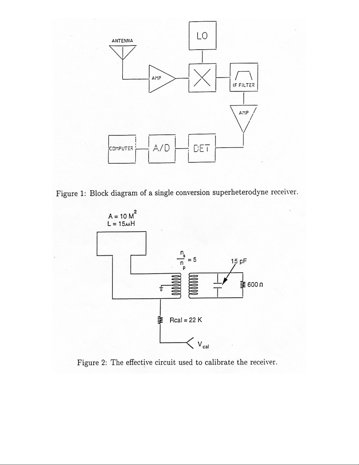
2 Radio Receiving General Principles

The basic components of a single-conversion superheterodyne receiver are shown in
Figure 1. An incoming signal is received by an antenna and amplified before reaching a
mixing stage. At the mixer, the received signal is multiplied or heterodyned with a known
local oscillator (LO) signal to establish an intermediate frequency (IF). In essence, it is
the LO frequency that tunes the receiver to the desired reception frequency. The IF
signal contains frequencies equal to the sum and difference of the frequencies of the LO
signal and the input signal from the antenna. The difference frequency is selected using a
tuned IF crystal filter. The resulting signal is amplified, detected, and digitized. There is
no need for an automatic gain control in our receivers since we are looking for absolute
signal strength and are not interested in keeping a constant output, as is typically
desirable in commercial receivers. Furthermore, receivers with two mixer stages
(double-conversion receivers) are also not desirable since the dynamic range of such a
receiver is usually downgraded through the addition of the second mixer.

1

2

3 Antenna and Preamplifier

The AGO LF/MF/HF receiver employs a magnetic loop antenna which is less susceptible
to locally generated noise than an electric dipole, especially when oriented to null out the
strongest local signal. The loop consists of a single turn of wire arranged in a square
between two vertical 12-foot-long 4 x4 posts placed 3 m apart. One horizontal wire
runs along the snow, and the other connects the tops of the posts, so that the area of the
loop antenna is 10 square meters. Figure 3 shows the antenna as deployed at AGO-P2.

The preamplifier is buried in the snow at the base of the antenna, with a pole or
flag installed to make it easy to retrieve. A schematic of the most recent version of the
preamplifier is included in the schematics portion of this manual. A critical component
of the preamplifier is the calibration circuit, which allows the absolute level of the
received signals to be calibrated. For this purpose, a broadband calibration signal
designed to be near the top of the instrument s range is injected approximately hourly.
This signal is detected by the receiver with its nominal gain, and then detected with the
gain reduced by 20 dB. Using both of these detections, the gain and offset of the
instrument can be accounted for, and the signals from the various AGO s can be
compared. Figure 2 shows the effective calibration circuit. (The 600-Ohm resistor
represents the input impedance of the preamplifier.)

The voltage at the antenna terminals of the loop antenna is related to the electric
field of the impinging EM radiation:

dE

A

V =

(1)

dt

c

where A is the antenna area (10 m2), E is the electric field strength, and c is the velocity
of light. Assuming that the antenna can be considered a perfect inductor at the
frequencies of interest,

dI

LV =

dt

(2)

where I is the current in the antenna, this leads to the following relation after integration

LI =

A

E

c

(3)

3