Agilent N8972A Quick Reference Guide

Download

Noise Figure Analyzers

NFA Series

Quick Reference Guide

Manufacturing Part Number: N8972-90003

May 2000

Safety Notices

This product and related documentation must b e reviewed for familiarization with safety markings and instructions before use.

This instrument has been designed and tested in accordance with IEC Publication 61010-1+A1+A2:1991 Safety Requirements for Electrical Equipment for Measurement, Control and Laboratory Use and has been supplied in a safe condition. The instruction documentation contains information and warnings which must be followed by the user to ensure safe operation and to maintain the instrument in a safe condition.

The information contained in this documentissubject to change without notice.

Agilent Technologies makes no warranty of any kind with regard to this material, including but not limited to, the implied warranties of merchantability and fitness for a particular purpose. Agilent Technologies shall not be liable for errors contained herein or for incidental or consequential damages in connection with the furnishing, performance, or use of this material.

The following safety symbols are used throughout this manual. Familiarize yourself with the symbols and their meaning before operating this instrument.

WARNING Warning denotes a hazard. It calls attention to a procedure

which, if not correctly performed or adhered to, could result in injury or loss of life. Do not proceed beyond a warning noteuntil the indicated conditions are fully understood and met.

CAUTION Caution denotes a hazard. It calls attention to a procedure that, if not

correctly performed or adhered to, could result in damage to or destruction of the instrument. Do not proceed beyond a caution sign until the indicated conditions are fully understood and met.

NOTE Note calls out special information for the user’s attention. It provides

operational information or additional instructions of which the user should be aware.

The instruction documentation symbol. The product is marked with this symbol when it is necessary for the user to refer to the instructions in the documentation.

This symbol is used to mark the on position of the power line switch.

This symbol is used to mark the standby position of the power line switch.

This symbol indicates that the input power required is AC.

WARNING This is a Safety Class 1 Product (provided with a protective

earthing ground incorporated in the power cord). The mains plug shall only be inserted in a socket outlet provided with a protected earth contact. Any interruption of the protective conductor inside or outside of the product is likely to make the product dangerous. Intentional interruption is prohibited.

WARNING If this product is not used as specified, the protection provided

by the equipment could be impaired. This product must be used in a normal condition (in which all m eans for protection are intact) only.

WARNING No operator serviceable parts inside. Refer servicing to qualified

personnel. To prevent electrical shock do not remove covers.

iii

WARNING For continued protection against fire hazard, replace line fuses

only with the same type and ratings (115V range; type F 5A 125V; 239V range F 5A 250V). The use of other fuses or materials is prohibited.

CAUTION To prevent electrical shock, disconnect the instrument from the mains

(line) before cleaning. Use a dry cloth or one slightly dampened with water to clean the external case parts. Do not attempt to clean internally.

Environmental requirements: This product is designed for indoor use only and to meet the following environmental conditions:

• Operating temperature: 0° Cto+55° C

• Operating humidity: <95% relative

• Altitude: up to 4500 m

Warranty

This Agilent Technologies instrument product is warranted against defects in material and workmanship for a period of three years from date of shipment. During the warranty period, Agilent Technologies Company will, at its option, either repair or replace products which prove to be defective.

Forwarranty service or repair,this product must be returned to a service facility designated by Agilent Technologies. Buyer shall prepay shipping charges to Agilent Technologies and Agilent Technologies shall pay shipping charges to return the product to Buyer. However, Buyer shall pay all shipping charges, duties, and taxes for products returned to Agilent Technologies from another country.

Agilent Technologieswarrantsthat its software and firmware designated

by Agilent Technologies for use with an instrument will execute its programming instructions when properly installed on that instrument. Agilent Technologies does not warrant that the operation of the instrument, or software, or firmware will be uninterrupted or error-free.

LIMITATION OF WARRANTY

The foregoing warranty shall not apply to defects resulting from improper or inadequate maintenance by Buyer, Buyer-supplied software or interfacing, unauthorized modification or misuse, operation outside of the environmental specifications for the product, or improper site preparation or maintenance.

NO OTHER WARRANTY IS EXPRESSED OR IMPLIED. AGILENT TECHNOLOGIES SPECIFICALLY DISCLAIMS THE IMPLIED WARRANTIES OF MERCHANTABILITY AND FITNESS FOR A PARTICULAR PURPOSE.

EXCLUSIVE REMEDIES

THE REMEDIES PROVIDED HEREIN ARE BUYER’S SOLE AND EXCLUSIVE REMEDIES. Agilent Technologies SHALL NOT BE LIABLE FOR ANY DIRECT, INDIRECT, SPECIAL, INCIDENTAL, OR CONSEQUENTIAL DAMAGES, WHETHER BASED ON CONTRACT, TORT, OR ANY OTHER LEGAL THEORY.

Where to Find the Latest Information Documentation is updated periodically. For the latest information about

Agilent NFA Noise Figure Analyzers, including firmware upgrades and application information, please visit the following Internet URL:

http://www.agilent.com/find/nf/

Manufacturer's Declaration

This statement is provided to comply with the requirements of the German Sound Emission Directive, from 18 January 1991.

This product has a sound pressure emission (at the operator position) < 70 dB(A).

• Sound Pressure Lp < 70 dB(A).

• At Operator Position.

•NormalOperation.

• According to ISO 7779:1988/EN 27779:1991 (Type Test).

Herstellerbeschein igung

Diese Information steht im Zusammenhang mit den Anforderungen der Maschinenlärminformationsverordnung vom 18 Januar 1991.

• Schalldruckpegel Lp < 70 dB(A).

•AmArbeitsplatz.

• Normaler Betrieb.

• Nach ISO 7779:1988/EN 27779:1991 (Typprüfung).

Contents

1. Getting Started

WhatYouwillFindinthisChapter..............................2

OverviewoftheFront-Panel....................................3

OverviewoftheRear-Panel.....................................6

DisplayAnnotation...........................................8

OverviewoftheFrontPanelKeys..............................11

HowtheFrontPanelKeysareOrganized ......................11

NavigatingThroughtheMenuSystem.........................11

PerformingCommonFileOperations............................13

FormattingaDiskette......................................13

SavingaFile..............................................15

LoadingaFile.............................................16

RenamingaFile...........................................16

CopyingaFile.............................................17

DeletingaFile ............................................18

WorkingwithTables.........................................19

2. Making Basic Measurements

WhatYouwillFindinthisChapter.............................22

EnteringENRData..........................................23

Selecting a Common ENR Table . . . . . . . . . .....................23

EnteringENRTableData...................................24

SavinganENRTable.......................................27

EnteringaSpotENRValue..................................28

ChangingtheDefaultTcoldvalue.............................28

SettingtheMeasurementFrequencies ..........................29

SelectingSweepFrequencyMode.............................29

SelectingListFrequencyMode...............................30

vii

Contents

SelectingFixedFrequencyMode............................. 32

SettingtheBandwidthandAveraging.......................... 33

SelectingaBandwidthValue................................33

SettingAveraging.........................................33

CalibratingtheAnalyzer.....................................34

Toperformacalibration....................................34

SelectingtheInputAttenuationRange........................ 35

DisplayingtheMeasurementResults...........................36

SelectingtheDisplayFormat................................ 36

SettingwhichResultTypesareDisplayed.....................38

Graphicalfeatures ........................................ 39

SettingtheScaling........................................41

WorkingwithMarkers.....................................43

IndicatinganInvalidResult..................................50

3. Advanced Features

WhatYouwillFindinthisChapter............................52

SettingupLimitLines.......................................53

CreatingaLimitLine......................................54

SettingLossCompensation...................................55

ConfiguringLossCompensation .............................55

4. Performing System Operations

WhatYouwillFindinthisChapter............................58

SettingtheGPIBAddresses..................................59

ToSettheGPIBAddresses..................................59

ConfiguringtheSerialPort................................... 60

ConfiguringtheLOGPIB .................................... 61

viii

Contents

ConfiguringtheCharacteristicsofanExternalLO ................62

CustomCommandSet......................................62

SettlingTime.............................................64

MinimumandMaximumFrequencies .........................65

ConfiguringtheInternalAlignment.............................66

TurningAlignmentOffandOn...............................66

ChangingAlignmentMode..................................66

DisplayingError,SystemandHardwareInformation..............67

DisplayingtheErrorHistory.................................67

DisplayingSystemInformation...............................67

DisplayingHardwareInformation ............................67

PresettingtheNoiseFigureAnalyzer...........................68

DefiningthePower-On/PresetConditions........................69

SettingthePowerOnConditions .............................69

SettingthePresetConditions................................69

RestoringSystemDefaults....................................70

SettingtheTimeandDate....................................71

Toturnthetimeanddateonandoff...........................71

Tosetthetimeanddate.....................................71

ConfiguringaPrinter ........................................72

ToConfigureaPrinter......................................72

TestingCorrectPrinterOperation ............................72

Contents

1 Getting Started

This chapter introduces you to basic features of the Noise Figure Analyzer, including front panel and rear panel descriptions, and an overview of the display annotation.

Getting Started

WhatYouwillFindinthisChapter

What You will Find in this Chapter

This chapter covers the following:

• Overview of the Front-Panel

• Overview of the Rear-Panel

• Display Annotation

• Overview of the Front Panel Keys

• Performing Common File Operations

• Working with Tables

2 Chapter1

Overview of the Front-Panel

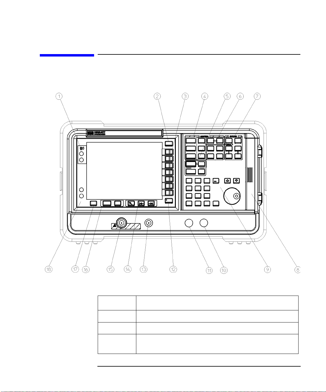
Figure 1-1 Front panel parts overview

Getting Started

Overview of the Front-Panel

Table 1-1 Front panel item descriptions

Item Description

1 Vie wing Angle keys allow you to adjust the display. 2The 3 Menu keys are the unlabeled keys next to the screen. The menu

Chapter 1 3

Esc (escape) key cancels any entry in progress.

key labels are shown on the display next to these unlabeled keys.

Getting Started

Overview of the Front-Panel

Table 1-1 Front panel item descriptions

Item Description

4TheMEASUREMENT functions allow you to configure the

measurement mode and set the NFA parameters needed for making measurements.

Frequency/Points and Averaging/Bandwidthkeysactivate

The the primary set up function keys and access menus of related functions.

Calibrate key r emoves any second stage noise contribution

The from the measurement. The from this menu, you can enter the ENR data.

Meas Mode and Mode Setup keys are used to configure the

The NFA to measure mixers and frequencies greater than the basic frequency of the NFA using a Local Oscillator.

ENR key accesses the ENR menu,

5The

DISPLAY functions allow you to configure the display

results.

6The

CONTROL functions control the NFA’s setup of Loss

Compensation

and input calibration ranges. The this group, as is full screen display. The

and Limit Line.TheCorr key sets correction

Sweep mode is controlled in

Full Screen functions in

all display formats.

SYSTEM functions affect the state of the Noise Figure Analyzer.

Various setup and alignment routines are accessed with the System key.

The green

Preset key resets the Noise Figure Analyzer to a

known state.

File key menu allows you to save and load traces, ENR

The tables, limit-line tables, and frequency lists to or from the NFA memory or the floppy disk drive. The

Save function defined under File.

the

Print Setup menu keys allow you to configure hardcopy

The output. The

Print key sends hardcopy data to the printer.

Save Trace key executes

8 The Media Door on the right side of the front panel accesses the

3.5 inch disk drive.

4 Chapter1

Table 1-1 Front panel item descriptions

Item Description

9 The Data Entry Keys, which include the Up/Down arrow keys,

RPG (rotatable knob), and numeric keys, allow you to enter or change the numeric value of an active function.

The RPG allows continuous change of functions such as, center frequency, averages, and marker position.

The Up/Down arrow keys allow discrete increases or decreases of the active function value.

Getting Started

Overview of the Front-Panel

⇐Prev key accesses the previously selected menu.

The 11 Not currently supported. 12 13

PROBE POWER provides power for other accessories.

NOISE SOURCE DRIVE OUTPUT +28V PULSED this

connector provides a 28 Vdc level to switch the noise source on.

The noise source is off when no voltage is applied. 14

Tab Keys are used to move between table input fields, and to

move within the fields of the dialog box accessed by the

menu keys. 15

INPUT 50ΩThis is the signal input connector for the Noise

Figure Analyzer. 16

The Next Window key selects which graph or result

parameter is active.

Pressing Zoom key while in graph mode allows you to

switch between the dual-graph and single-graph to display the

active graph. 17 Press the

Help key and then any front panel or menu key to get a

short description of the key function and the associated remote

command.

File



18 The

(On) key turns the Noise Figure Analyzer (NFA) on, while

O (Standby) key switches the NFA to standby.

the

Chapter 1 5

Getting Started

Overview of the Rear-Panel

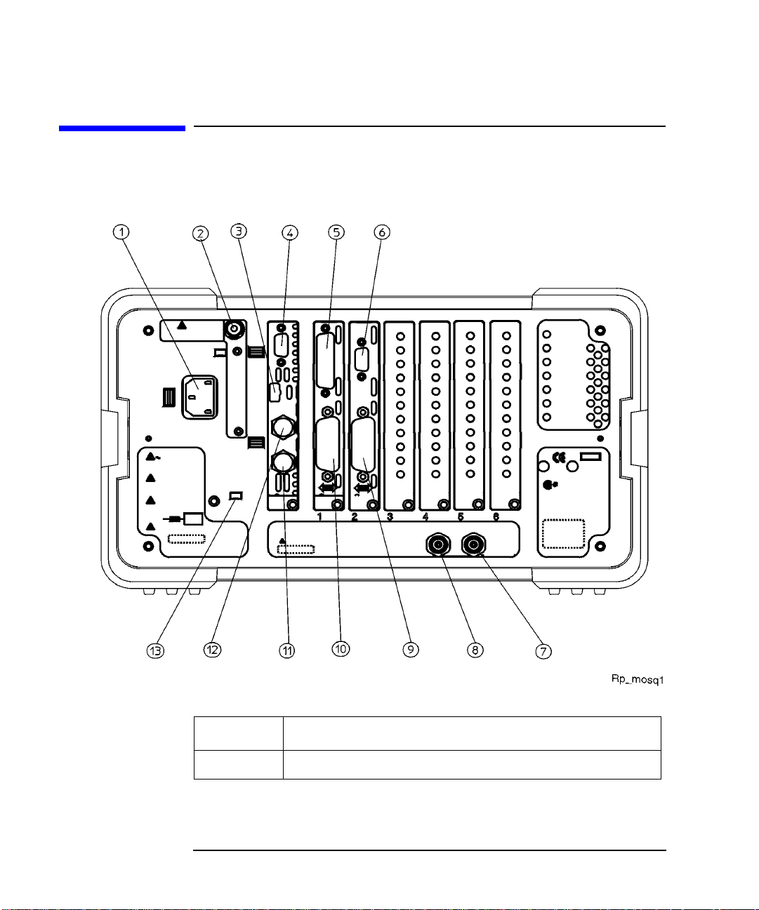
Figure 1-2 Rear panel parts overview

Table 1-2 Rear panel item d escriptions

Item Description

6 Chapter1

Power input is the input for the AC line-power source.

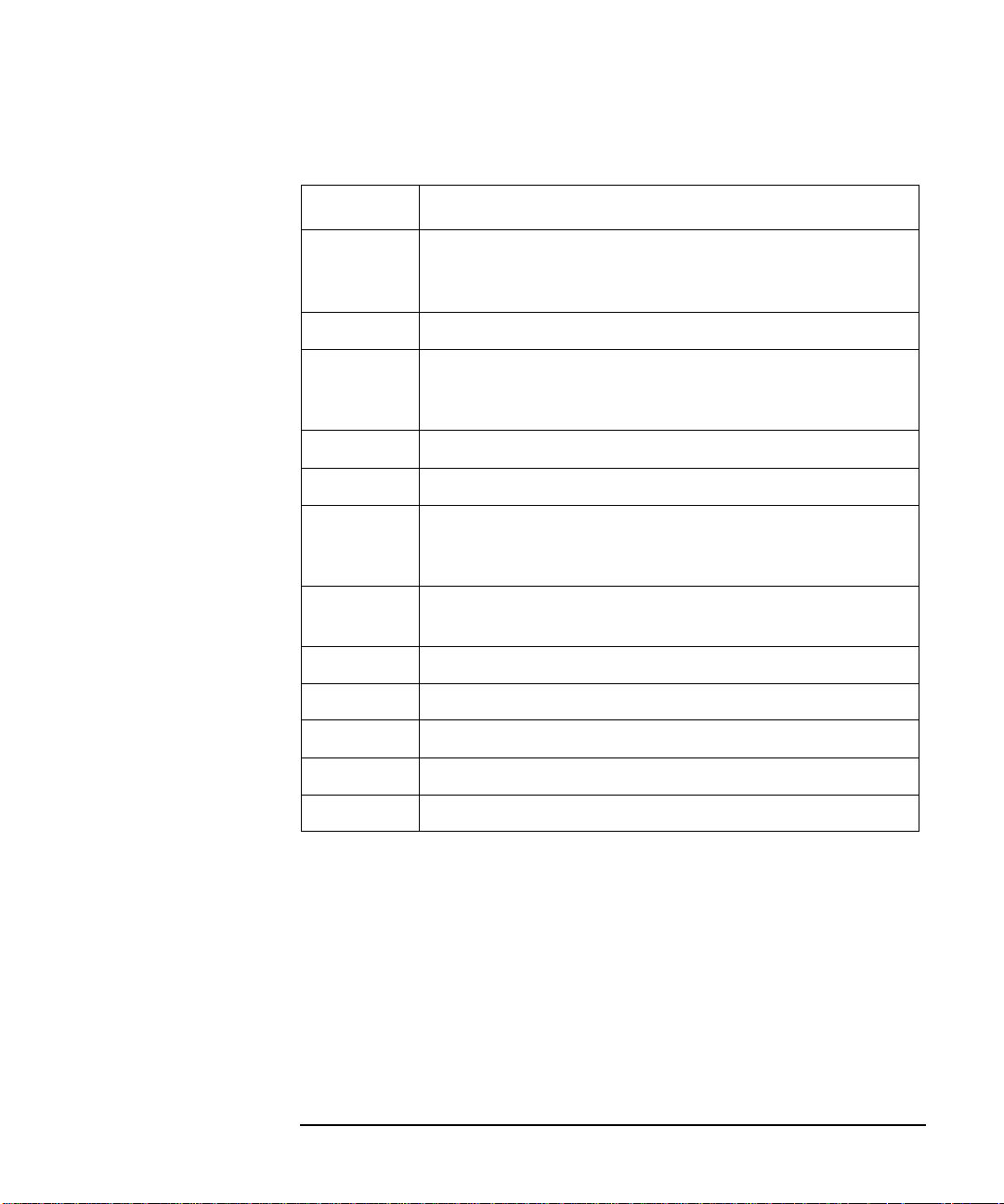
Table 1-2 Rear panel item d escriptions

Item Description

2 Line Fuse.Thefuseisremovedbytwistingcounterclockwise

1/4 turn. Replace only with a fuse of the same rating. See the

label on the rear panel. 3 Service Connector. The service connector is for service use only.

Getting Started

Overview of the Rear-Panel

VGA OUTPUT drives an external VGA compatible monitor with

a signal that has 31.5 kHz horizontal, 60 Hz vertical

synchronizing rate, non-interlaced. 5 6 7

PARALLEL interface parallel port is for printing only.

RS-232 interface supports remote instrument operation.

10 MHz REF IN accepts an external frequency source to provide

the 10 MHz, −15 to +10 dBm frequency reference used by the

Noise Figure Analyzer. 8

10 MHz REF OUT provides a 10 MHz, 0 dBm minimum,

timebase reference signal. 9 10 11 12

LO GBIB port is for the control of an external LO by the NFA.

MAIN GPIB interface port supports remote instrument operation.

AUX OUT (TTL) it is not currently supported.

AUX IN (TTL) it is not currently supported.

13 Power On Selection selects an instrument power preference.

Chapter 1 7

Getting Started

Display Annotation

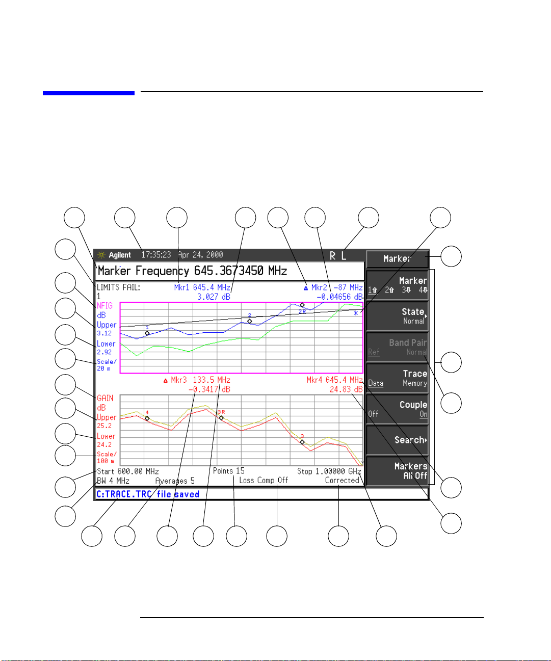
The graph display annotation, shown in Figure 1-3, is referenced by numbers, which are listed with a description and a function key indicating which key activates the function related to the annotation.

Figure 1-3 Display Ann otation

29 28

27 26

25 24

2 3 4 65 7 8

14151617181920

Each item is given a description and where applicable a function key associated with it.

8 Chapter1

Table 1-3 Display annotation item descriptions

Item Description

1 The active function area displays the label and value of the

currently active key.

Getting Started

Display Annotation

2 The time and date display, controlled by the

key, under the

System key menus.

3 The marker 1 frequency, controlled by the

State menu keys.

Time/Date menu

Marker(1⇑ ) and

4 The marker 1 amplitude. 5 The marker 2 frequency, controlled by the

State menu keys.

Marker(2⇑ ) and

6 The marker 2 amplitude. 7 The GPIB annunciators RLTS. 8 The data invalid indicator appears when a measurement starts. It

disappears after a complete sweep. 9 The key menu title, this is dependent on which key is selected. 10 The key menu. 11 A non-active menu key. 12 The marker 4 frequency,controlled by the

Marker(4⇓)and State

menu keys. 13 The marker 4 amplitude. 14 The frequency span or stop frequency, controlled by the

Span

or Stop Freq key.

Freq

15 Displays whether the measurement is corrected or uncorrected,

controlled by the calibration state and the

Corr key.

16 Displays whether Loss Compensation is On or Off, controlled

Loss Comp key.

by the 17 The number of points, controlled by the

Points menu key.

Chapter 1 9

Getting Started

Display Annotation

Table 1-3 Display annotation item descriptions

Item Description

18 The marker 3 frequency, controlled by the Marker(3⇓)and State

menu keys. 19 The marker 3 amplitude. 20 The number of averages, controlled by the

Averages menu key.

21 The display status line, displays instrument status and error

messages. 22 The bandwidth, controlled by the

Bandwidth menu key.

This is fixed at 4 MHz on the N8972A model. 23 The center frequency or start frequency, controlled by the

Center Freq or Start Freq menu keys.

24 The lower trace scale, controlled by the

Scale/Div menu key.

(This is auto-coupled to 25 and 26.) 25 The lower trace lower limit, controlled by the

Lower Limit menu

key. (This is auto-coupled to 24 and 26.) 26 The lower trace upper limit, controlled by the

Upper Limit menu

key. (This is auto-coupled to 24 and 25.) 27 The lower trace result type, controlled by the 28 The upper trace scale, controlled by the

Result menu key.

Scale/Div menu key.

(This is auto-coupled to 29 and 30.) 29 The upper trace lower limit, controlled by the

Lower Limit menu

key. (This is auto-coupled to 28 and 30.) 30 The upper trace upper limit, controlledbythe

Upper Limit menu

key. (This is auto-coupled to 28 and 29.) 31 The upper trace result type, controlled by the

Result key.

32 The limit line failure indicator.

10 Chapter1

Getting Started

Overview of the Front Panel Keys

How the Front Panel Keys are Organized

The front panel keys are divided into four main groups:

MEASURE keys, w hich are used to configure the measurement

• parameters

CONTROL keys, which are used to configure advanced measurement

• parameters

SYSTEM keys, which perform system-level operations

•

DISPLAY keys, which adjust the display characteristics of the

• measurement

Navigating Through the Menu System

Menu keys Pressing any of the grey front panel keys in the MEASURE, DISPLAY,

RESULT or SYSTEM key groupings accesses menus of functions that are

displayed along the right-hand side of the display. These keys are called menu keys. See Figure 1-4.

Chapter 1 11

Getting Started

Overview of the Front Panel Keys

Figure 1-4 Menu Keys

Action keys Pressing any of the white keys (

and Print) invokes an action and these keys are called action keys.

To activate a menu key function

To activate a menu key function, press the key immediately to the right of the screen menu key. The menu keys that are displayed depend on whichfrontpanelkeyispressedandwhichmenulevelorpageis selected.

Selecting a function within a menu key

Some menu keys have functions contained within them, for example, and Off. To turn the function on, press the menu key so that On is underlined. To turn the function off, press the menu key so that Off is underlined.

For a summary of all front panel keys and their related menu keys, see theUser’sGuideortheanalyzeronlinehelp.

12 Chapter1

Calibrate, Full Screen, Restart, Save Trace

Getting Started

Performing Common File Operations

This section covers:

• Formatting a diskette

• Saving a file

•Loadingafile

• Renaming a file

• Coping a file

• Deleting a file

FormattingaDiskette

The format is MS-DOS. It is not necessary to format your diskette with the Noise Figure Analyzer; pre-formatted disks can be used with the NoiseFigureAnalyzer.

Step 1. Place the diskette you wish to format into the diskette drive (A:\) of the

NoiseFigureAnalyzer.

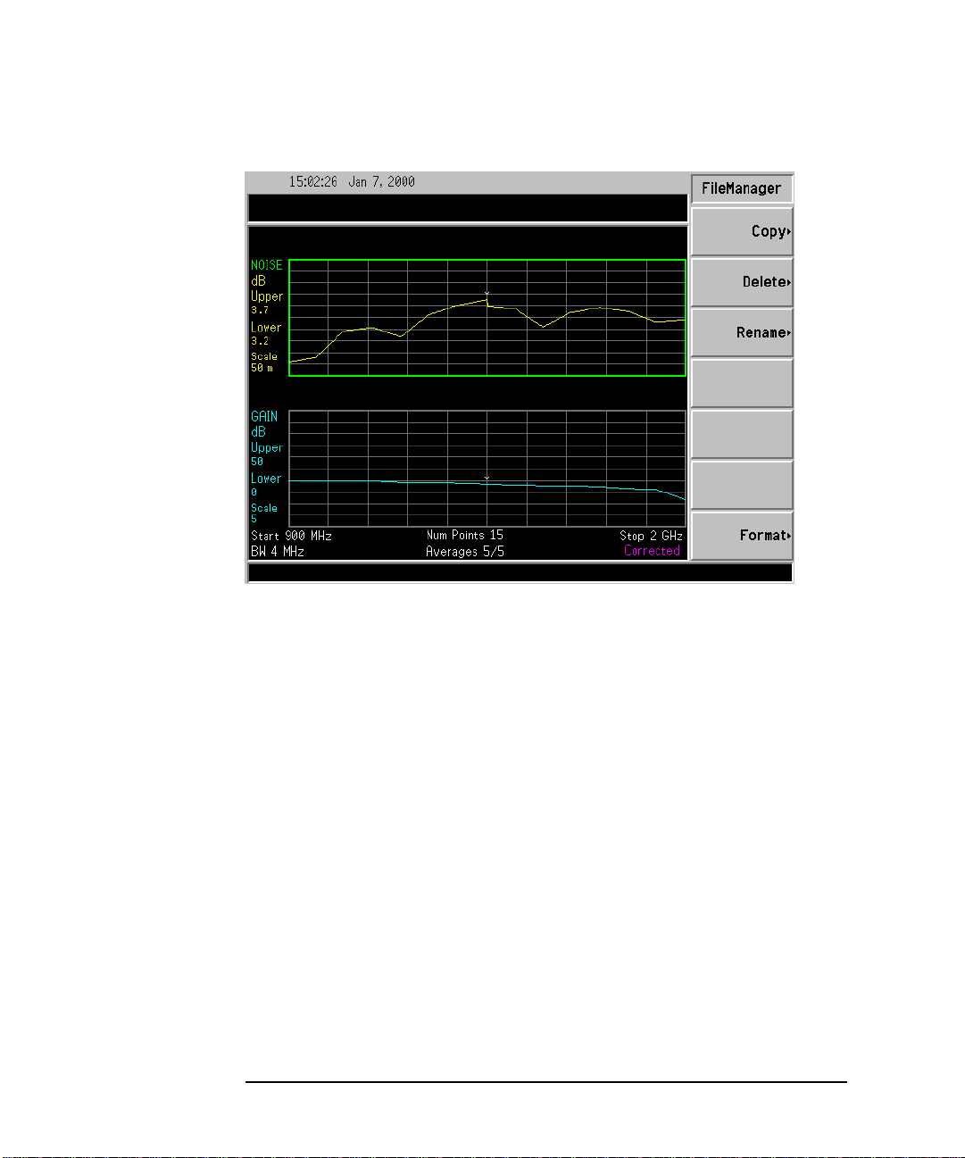
Step 2. Access the file manager menu by pressing

Figure 1-5.

Chapter 1 13

File key, File Manager.See

Getting Started

Performing Common File Operations

Figure 1-5 File Manager Menu

Step 3. Start the format process by pressing Step 4. Press

Enter, a second time to format the disk.

The format process takes approximately three minutes. You are now ready to save files to the disk.

14 Chapter1

Format,thenEnter.

Getting Started

Performing Common File Operations

SavingaFile

You can save files (ENR tables, states, traces, limits, frequency lists, or screens) to a floppy disk (A:\), or the internal drive (C:\)oftheNoise Figure Analyzer.

Step 1. To access the Save menu press

File, Save.

Step 2. Selectthetypeoffileyouwanttosave.

For example, if you have a limit line table data present and want to save it, press

Step 3. Select the limit tables file you wish to save (

Forexample,tosavefile2,press

Limits.

1, 2, 3 or 4).

Step 4. Enter a filename using the Alpha Editor menu keys. See“Using the

Alpha Editor” on page HIDDEN. File names are limited to eight (8) characters.

Step 5. Selectthedriveyouwishtosavetobypressing

directory and file list, press

Select.

Tab →,tomoveto

NOTE If the correct drive is not listed in the Path: field, highlight “..” at the

top of the directory list. This enables you to move up a directory. Press

Select. To highlight the desired drive,[-A-] or [-C-])usethearrowkeys

or the RPG, press Select when highlighted.

Step 6. Press

Enter,tosavethefiletothedrive.

Chapter 1 15

Getting Started

Performing Common File Operations

Loading a File

You can load files (ENR tables, states, limits or frequency lists) from a floppy disk (A:\), or the internal drive (C:\).

NOTE Not all the file types you save can be loaded back into the Noise Figure

Analyzer. For example, screen files and trace files. The trace file is in a CSV (comma separated value) format, designed for use with a PC.

Step 1. To access the Load menu press

File, Load.

Step 2. Select the type of file you want to load (ENR tables, states, limits or

frequency lists).

Step 3. Selectthedrivewhereyourfileislocatedbypressing

to highlight [-C-] or [-A-],thenpress

Select.

Tab →.UsetheRPG

Step 4. Select the file you want to load into the Noise Figure Analyzer by

changing the highlighted file with the up or down arrow keys to highlight the file name.

Step 5. Press

Enter to load the specified file.

Renaming a File

You can rename a file in the [-C-] or [-A-] drive as follows:

Step 1. Press Step 2. Select the type of file you want to rename (ENR tables, states, traces,

Step 3. Select the drive where you file is located, by pressing the

File, File Manager, Rename toaccesstheRenamemenuitems.

limits, frequency lists or screens). For example, if you are renaming a ENR table file, press

Select.Tochangedrive,usethearrowkeystohighlight[-C-] or [-A-],

then press

Select.

ENR. Tab →key, press

Step 4. Select the file you want to rename by moving the cursor with the RPG or

arrow keys to highlight the file name.

Step 5. Press

Tab →to enter the Alpha Editor menu. File names are limited to

eight (8) characters.

16 Chapter1

Getting Started

Performing Common File Operations

Step 6. Press Enter and your file is now renamed and visible within the directory

displayed on your Noise Figure Analyzer.

Copying a File

This allows you to copy a file to a different location on both the [-C-] and [-A-] drive.

Step 1. To access the Copy menu press

File, File Manager, Copy.

Step 2. Put a formatted floppy in the A: drive. Step 3. Select the type of file you want to rename (ENR tables, states, traces,

limits, frequency lists or screens. For example, if you are copying a State file, press

Step 4. Select the drive where your file is located, by pressing

State.

Tab → to highlight

the From:Path: field. Select the drive, using the RPG or arrow keys to highlight [-C-] or [-A-],thenpress

Select.

Step 5. Select the file you wish to copy by highlighting the filename using the

front-panel knob or arrow keys.

Step 6. Press

Tab →to move to the To:Path: field and select the drive where you

want to copy the file using the RPG or arrow keys then press

Select.

NOTE If the correct drive is not listed in the Path: field, highlight “..” at the

top of the directory list. This enables you to move up a directory. Press

Select, to highlight the desired drive, ([-A-] or [-C-])thenpressSelect

again.

Step 7. Copythefilebypressing

Chapter 1 17

Enter.

Getting Started

Performing Common File Operations

DeletingaFile

This allows you to delete a file from the [-C-] or [-A-] drive.

Step 1. To access the Delete menu press

File Setup, File Manager, Delete.

Step 2. Select the type of file you want to delete (ENR tables, states, traces,

limits, frequency lists or screens).

Step 3. Select the drive where the file you wish to delete is located, by pressing

Tab →then press using the RPG or arrow keys to highlight [-C-] or

[-A-],thenpress

Select.

NOTE If the correct drive is not listed in the Path: field, highlight “..” at the

top of the directory list. This enables you to move up a directory. Press

Select, to highlight the desired drive, ([-A-] or [-C-])thenpressSelect

again.

Step 4. Select the file you want to delete by moving t he cursor with the RPG or

arrow keys to highlight the file name.

Step 5. Press

Enter and your file is now deleted and is no longer visible in the

directory displayed on your NFA.

18 Chapter1

Working with Tables

The Frequency List, ENR Table and Limit Line Editor use table forms. The following is an overview of how to use the common features in these

tables.

Table 1-4 Using Tables

To... Use the...

Getting Started

Working with Tables

Move the highlight bar within the table Bring the highlight bar to the top of the

Tab keys Home key

table Clear the table of all entries Delete a single row entry Add a new entry

Move the highlight bar up one row Move the highlight bar down one

Clear Table menu key Delete Row menu key Add menu key Row Up menu key Row Down menu key

row Move the table up a page block

Move the table down a page block

Page Up menu key Page Down menu key

Enter a value Numerical key pad Terminate a value The unit values presented by the

menu keys

Connect Limit Line points The arrow keys or the RPG

a. A limit line value is a limit less value where it depends on the

result scale used. To terminate use th e scale linear termination menu keys.

Chapter 1 19

Getting Started

Working with Tables

20 Chapter1

2 Making Basic Measurements

This chapter describes how to make basic noise figure measurements using y our Noise Figure Analyzer and a lso covers the most common measurement related tasks.

Making Basic Measurements

WhatYouwillFindinthisChapter

What You will Find in this Chapter

This chapter covers:

•EnteringENRData

• Setting the Measurement Frequencies

• Setting the Bandwidth and Averaging

• Calibrating the Analyzer

• Displaying the Measurement Results

• Example of How to Make a Basic Amplifier Measurement

22 Chapter2

Making Basic Measurements

Entering ENR Data

You can enter ENR data for the noise source you are using as a table for measurements at several frequencies, or a s a single spot value for measurements at a single frequency.

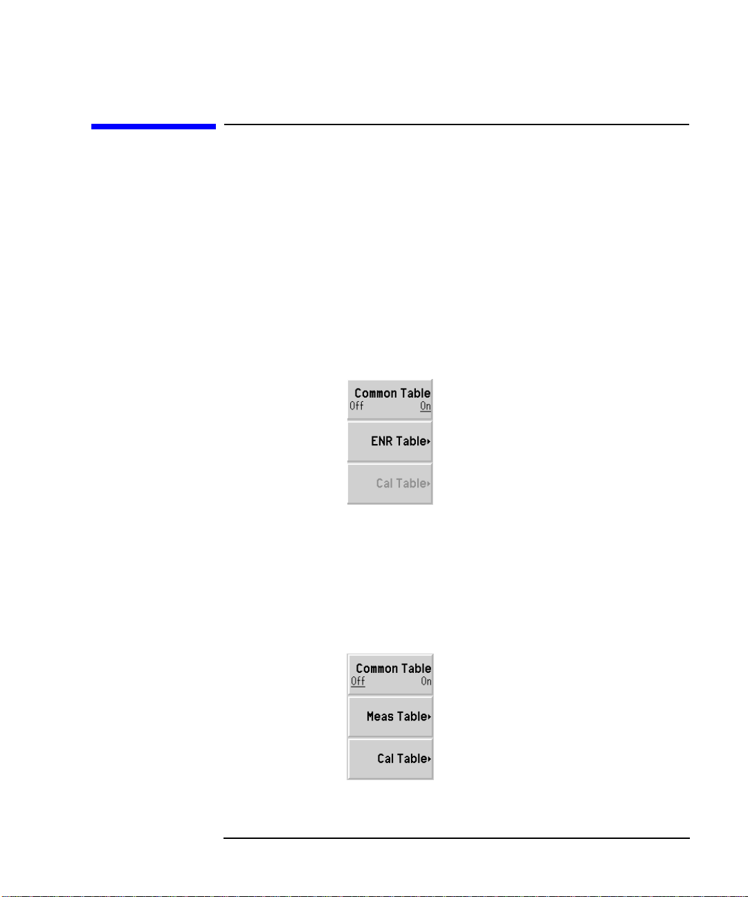
Selecting a Common ENR Table

To use the same ENR table for calibration and measurement, press the

Common Table menu key set the Common Table(On),seeFigure2-1.

This is the default setting. In this mode the

Figure 2-1 Menu Keys showing Common ENR Table Enabled

To use different ENR tables for calibration and measurement, press the

Common Table menu key set the Common Table(Off), see Figure 2-2.

In this mode, the of the noise source used to calibrate the Noise Figure Analyzer. The

Table

is used to make the measurements.

Figure 2-2 Menu Keys showing Common ENR Table Disabled

Cal Table menu key is accessible. This is the ENR table

Cal Table is not accessible.

Meas

Chapter 2 23

Making Basic Measurements

Entering ENR Data

Entering ENR Table Data

You can enter ENR data in the form of an ENR table in four ways:

• manually by inputting the required frequencies and corresponding ENR values

• loading the ENR data from a diskette, on which the data has been previously stored

• loading the ENR data from the internal memory, where the data has been previously stored

• loading of the ENR data using t he GPIB Programmer, see the Programmer’s Guide for more details

To enter ENR table data manually

Step 1. Press the

Figure 2-3 An Empty ENR Table

Step 2. Optional Step

Press the number using the numeric keys and the Alpha Editor.

ENR key, and the ENR Table menu key.

Serial Number menu key and enter the noise source serial

24 Chapter2

Step 3. Optional Step

Making Basic Measurements

Entering ENR Data

Press the

ID menu key and enter the noise source model number using

the numeric keys and the Alpha Editor.

Step 4. Press the

Edit Table menu key to enter the noise source ENR values.

Step 5. Enter the first frequency using the num eric keys in the table using the

unit termination menu keys.

Step 6. Press the

Tab —> key to move the highlight to the ENR Value column and

enter the corresponding ENR value of the ENR list. When terminating the ENR value you can use either

dB, K, C,orF menu

keys. However, the result which appears in the table is in dB.

Step 7. Press the

Tab —> key to move the highlight to the Frequency column and

enter the next frequency value on the ENR l ist.

Step 8. Repeat steps 5 to 7 and until all the frequency and ENR values you need

are entered.

Step 9. After completing the ENR table entries, press the

Prev key or ENR key to

return to the ENR menu.

Step 10. Once you have completed entering the ENR data, save the ENR table

using the

File key.

Chapter 2 25

Making Basic Measurements

Entering ENR Data

Figure 2-4 A Typical ENR Table after data entry

NOTE If you do not save the ENR table, it is lost the next time you power down

or preset the instrument, as the data is temporarily stored in volatile memory. This is overcome if you use

Power On(Last) or Preset(User) which

contains an ENR table.

26 Chapter2

Making Basic Measurements

Entering ENR Data

To load ENR data from memory

Step 1. If the ENR file is on diskette, insert the diskette into the floppy drive of

the Noise Figure Analyzer.

Step 2. Press the Step 3. Press the Step 4. Press the

File key to access the File Manager. Load menu key to access the file system. ENR menu key.

Step 5. Press either the

A list of available files on the [-A-] or [-C-] drive is displayed. Use the arrow keys to access the appropriate file.

Step 6. Press the

Enter key.

Saving an ENR Table

You can save an ENR table to the Noise Figure Analyzer’s internal memory or to floppy disk as follows:

Step 1. Press the Step 2. Press the Step 3. Press the Step 4. Press either the

The

File key. Save menu key. ENR menu key.

Alpha Editor now appears, allowing you to create a name for the file.

Meas Table or Cal Table menu key.

Step 5. Input the name of the ENR table. Step 6. Select using the arrow keys whether you want to save the files to the

[-A-] or [-C-] drive.

Step 7. Press

Enter to terminate.

Chapter 2 27

Making Basic Measurements

Entering ENR Data

Entering a Spot ENR Value

To enter a Spot ENR value:

Step 1. Press the

ENR key, then the Spot ENR menu key.

Step 2. Enter an ENR value using the numeric keys and terminate it using the

unit termination menu keys. The default value is 15.20 dB.

NOTE If the frequency you want to measure is not a listed ENR value, then you

need to interpolate the ENR list to an appropriate value.

NOTE To enable spot ENR mode to operate, press the ENR key, and select the

ENR Mode(Spot) menu key.

Changing the Default T

cold

value

When working in different temperature conditions you can change the

valuetoaccommodatethecondition.

cold

To change the T

Step 1. Press the

ENR key.

cold

value:

Step 2. Press the

Tcold(On).

Step 3. Press the

Enter a T unit termination menu keys. The default T

The unit termination menu keys are in

F (Fahrenheit).

28 Chapter2

Tcold menu key changing it from the default Tcold(Off) to

User Tcold menu key

value using the numeric keys and terminate it using the

cold

value is 296.5K.

cold

K (Kelvin), C (Celsius) or

Making Basic Measurements

Setting the Measurement Frequencies

Three frequency modes are available:

Sweep — the measurement frequencies are obtained from the start

• and stop (or equivalent center and span) frequencies and the number

of measurement points.

List — the measurement frequencies are obtained from the frequency

• list entries.

Fixed — where the measurement frequency is taken at single fixed

• frequency.

Selecting Sweep Frequency Mode

NOTE You can press Full Span at anytime to return the frequency range to the

default full range setting. If you do this after a calibration and the calibration has been made over a narrower frequency range, it invalidates the calibration.

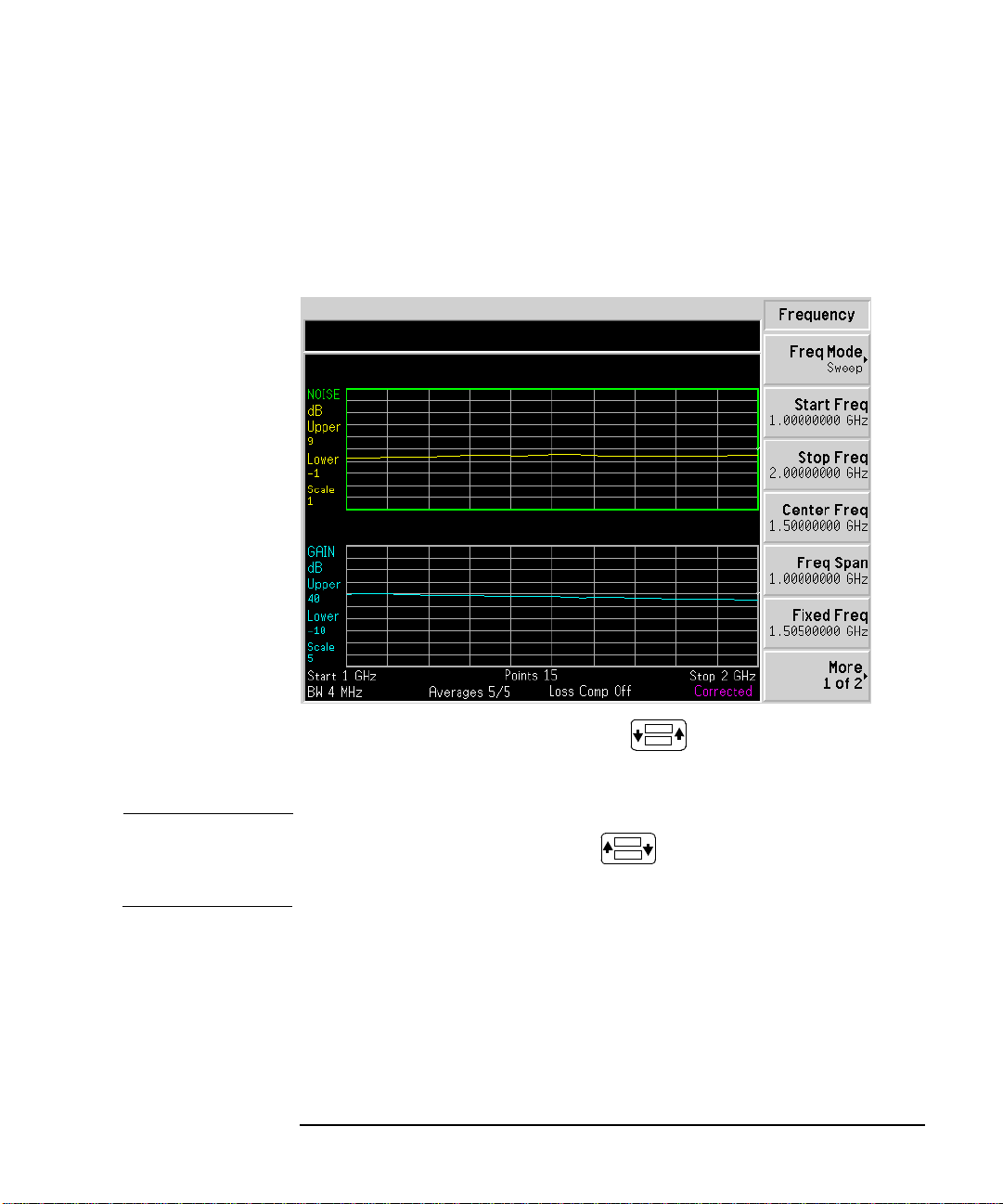
Step 1. Press the Step 2. Press the

Freq Mode(Sweep).

Chapter 2 29

Frequency/Points key. Freq Mode menu key and set the frequency mode to

Making Basic Measurements

Setting the Measurement Frequencies

Step 3. Enter the frequency range by either entering the Star t Freq and Stop Freq

frequencies, or the Center Freq and the Freq Span.

Step 4. Press the

More 1 of 2, Points menu keys.

Step 5. Enter the number of measurement points using the numeric keys to

enter the number, press the

Enter key to terminate.

Selecting List Frequency Mode

You can create a frequency list in the following ways:

• Manually, by specifying each individual point

• From s weep points, by specifying the measurement frequency range and setting the Noise Figure Analyzer to generate equally spaced points within that range, using the

• Loading a list from the internal memory or diskette, where the data has been previously stored.

• Loading a list using the G PIB Programmer, see the Programmer’s Guide if you want to use this method.

To Create a Frequency List Manually

Step 1. Press the Step 2. Press the

Frequency/Points key and press the More 1 of 2 menu key. Freq List menu key.

Fill menu key.

30 Chapter2

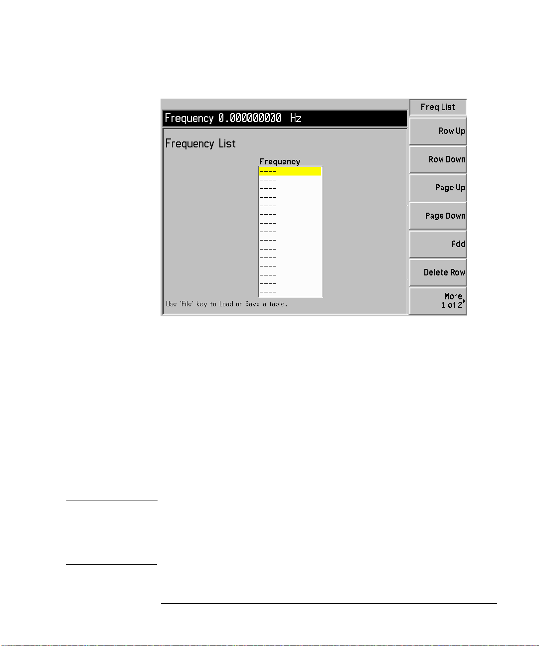
Figure 2-5 An Empty Frequency List

Making Basic Measurements

Setting the Measurement Frequencies

Step 3. Press the

More 1 of 2, Clear Table menu keys.

Step 4. Enter the frequency value you want using the numeric keys. Terminate

it using the unit menu keys which are presented to you.

Step 5. Press the

Tab —> key or Row Down menu key.

Enter the next frequency value of the frequency list b y using the numeric key pad and the unit termination keys.

Step 6. Repeat step 5 until your list is complete. Step 7. Save the Frequency List to the Noise Figure Analyzer internal memory

or to a diskette if required using the

File key.

NOTE Youneedtosavethefrequencylistoritislostifyoupowerdownthe

instrument, as the data is temporarily s tored in volatile memory. This is overcome i f you use

Power On(Last) or Preset(User) which contains a

Frequency List.

Chapter 2 31

Making Basic Measurements

Setting the Measurement Frequencies

Creating a Frequency List from Swept Points

When you have a series of swept frequency points and you want to create a frequency list from them, press the

More 1 of 2, Fill menu keys. This

clears the current frequency list and fills the list with the frequencies generated by the sweep frequency mode.

Selecting Fixed Frequency Mode

The fixed frequency mode is used when you want to make a measurement at a single frequency.

To set a fixed frequency:

Step 1. Press the Step 2. Press the

Frequency/Points, Freq Mode menu keys. Fixed menu key to set the frequency mode to Freq Mode(Fixed).

Step 3. Enter the frequency value using the numeric keys and the unit

termination menu keys.

32 Chapter2

Setting the Bandwidth and Averaging

Selecting a Bandwidth Value

Step 1. Press the Averaging/Bandwidth key.

Making Basic Measurements

Setting the Bandwidth and Averaging

The current bandwidth is shown on the

Step 2. Press the

the list of available options.

NOTE This feature is not applicable to N8972A. The bandwidth is fixed at

4MHz.

Bandwidth menu key and select the bandwidth you want from

Bandwidth menu key.

Setting Averaging

Increased averaging reduces jitter and provides smoother display traces. However, the measurement speed is sacrificed.

Enabling averaging

Averaging can be enabled by setting the averaging set

Selecting the Number of Averages

Step 1. Press the Step 2. Enter the numeric val ue you want using the numeric key pad. Terminate

it with the

Averaging(Off)

Averaging/Bandwidth key,andthentheAverages menu key.

Enter key.

Averaging(On). To disable

Setting the Averaging Mode

Averaging Mode can be set to

Average Mode(Sweep).

NOTE The N8972A only functions in point average mode.

Chapter 2 33

Average Mode(Point) or

Making Basic Measurements

Calibrating the Analyzer

Calibration is necessary to compensate for the noise contribution of the Noise Figure Analyzer and any associated cabling etc. in the

measurement path. To perform calibration you need to enter the ENR values and set up the

frequency range, number of measurement points, bandwidth and the averaging used for the measurement. For more details on calibration, such as when to perform calibration and when calibration is invalidated etc. see the User’s Guide.

To perform a calibration

Step 1. Input the ENR values of the noise source into the Noise Figure Analyzer,

or verify that the correct ENR table is loaded. See “Entering ENR Data” on page 23 for more details.

Step 2. Configure the measurement parameters (frequency range, number of

points, bandwidth and averages) you want to use for the measurement.

Step 3. Connect the noise source output directly to the Noise Figure Analyzer

input.

Figure 2-6 Noise Figure Analyzer Calibration

Noise Source

NOTE You need an adapter on the Noise Figure Analyzer input unless the noise

source is an Agilent 346B Option 001 (Type N male) output connector.

34 Chapter2

Making Basic Measurements

Calibrating the Analyzer

Step 4. If required select an input attenuator range by pressing the Corr key and

Input Cal menu key to set the minimum and maximum input

the attenuation.

See “Selecting t he Input Attenuation Range” on page 35 for mode details on input attenuation.

Step 5. Press the

Calibrate key twice to initiate the calibration.

Selecting the Input Attenuation Range

When measuring a high-gain device you need to increase the input attenuation. If you do not know the gain of the DUT, you can perform calibration using the default range, note what error codes are presented and then calibrate again using the greater attenuation values. If the Noise Figure Analyzer continues to display error codes, there is a need to add external attenuator pads and correct for this using the Loss Compensation. This is explained in “Setting Loss Compensation” on page 55.

If an error message occurs while calibrating, you need to recalibrate. For a complete list of error codes see the User’s Guide.

To select the input attenuation:

Step 1. Press the Step 2. Press the Step 3. Set the attenuator range using the

and select the attenuation values you want from the list.

Corr (Corrected) key. Input Cal menu key and select the attenuation range you want

Min Atten and Max Atten menu keys,

Chapter 2 35

Making Basic Measurements

Displaying the Measurement Results

The following display format features are available:

• Graph, Table or Meter mode display

• Single or dual-graph display allowing any two available result types to be displayed simultaneously

• Zoom to display only one result graph on the display

• Combineoptiontodisplaytworesulttypesonthesamegraph

• Markers for searching the trace

• Display a live trace, a memory trace or both

• Save the current trace data to memory

• Switch the graticule on or off

• Switch display annotation on or off

Selecting the Display Format

You can display the measurement results in either:

• Graph format

• Table format

• Meter format.

To set the display format:

Step 1. Press the Step 2. Press the

to select the display mode you want.

36 Chapter2

Format key. Format menu key and select the Graph, Table or Meter menu key

Making Basic Measurements

Displaying the Measurement Results

Navigating Around the Display

Active Graph The active graph is highlighted by a green border. Noise Figure is the

active graph by default.

Figure 2-7 Dual-graph display

Changing the Active Graph

NOTE When in table or meter format the key changes the active

Tochange the active graph, press the key below the display. This key allows you to set the upper or lower graph as the active graph.

parameter.

Chapter 2 37

Making Basic Measurements

Displaying the Measurement Results

Viewing the Full Screen

You can fill the entire display and remove the menu keys and certain annotation from the display. Press the

screen. Pressing the

Full Screen key again returns it to a previous display.

Full Screen key to view the full

NOTE The Full Screen key also functions in table or meter format.

Setting which Result Types are Displayed

To specify which measurement results are displayed

Step 1. Press the Step 2. Select the Format by pressing the appropriate menu key.

Step 3. Select which result is active, using the key. Step 4. Press the

Step 5. Press the key to make the other measurement parameter active. Step 6. Press the

Format key, then the Format menu key

Result key a nd select the result type that you want to display.

Result key a nd select the result type you want to display.

NOTE When you press the Scale key, the active result for the selected

parameter is shown.

38 Chapter2

Graphical features

Viewing a single graph

While in graph format mode, you can press the key located below the display and the active graph fills the display as a single graph.

Figure 2-8 Displaying a single graph

Making Basic Measurements

Displaying the Measurement Results

Combining the two graphs on the same graph

The default setting is To combine the two graphs:

Step 1. Press the Step 2. Press the

graphs on the same graph.

Chapter 2 39

Combined(Off) and the graphs are not combined.

Format key and ensure Format(Graph) is selected. Combined(On) menu key to combine the two currently displayed

Making Basic Measurements

Displaying the Measurement Results

Figure 2-9 Typical display with two tr aces combined on the same graph

Displaying the Current Data Trace and the Recalled Memory Trace

When a trace finishes its first complete sweep the

Data -> Memory menu

key becomes enabled. To save a trace to memory, press the

pressing the

Data -> Memory menu key, the Trace menu key becomes

Data -> Memory menu k ey. After

active. To view the saved trace, press the

Memory menu key. The recalled trace is presented in the display.

Toview both the saved trace and the current active trace, press the

Trace menu key, followed by the

Trace

menu key, followed by the Data & Memory menu key. Toview the current data trace only, press t he

Data menu key. This is the default setting.

the

Trace menu key, followed by

40 Chapter2

Displaying the Measurement Results

Turning the Graticule On and Off

To turn the graticule on or off:

Making Basic Measurements

Step 1. Press the Step 2. Press the

required.

Turning the Display Annotation On or Off

To turn the annotation on or off:

Step 1. Press the Step 2. Press the

required.

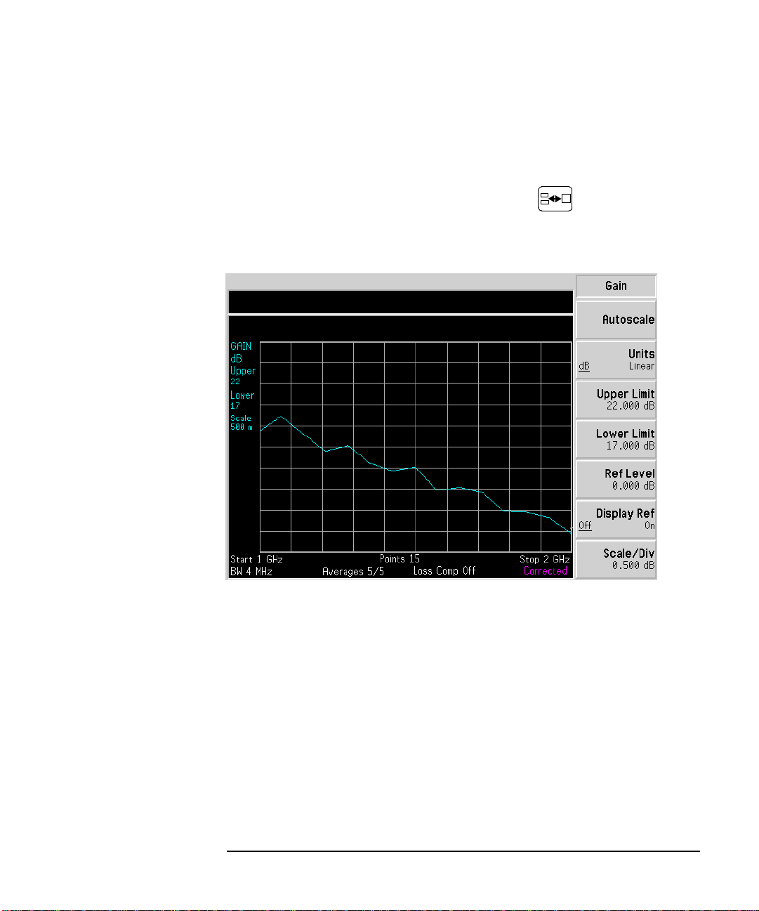
Setting the Scaling

You can set the result’s scale parameters in the active graph. To set the scale, press the

To change the active graph, press the measurement parameter’s menu key. Press the of the selected measurement parameter.

You can set the scale for the measurement parameter or press the

Autoscale menu key. Pressing Autoscale selects the optimum values for

Upper Limit, Lower Limit, and Scale/Div.

Format key.

Graticule menu key to set it to the Graticule(Off) or Graticule(On) as

Format key.

Annotation menu key to set it to Annotation(Off) or Annotation(On) as

Scale key.

Result key and select another

Scale key to set the scale

NOTE When Autoscale is pressed and limit lines are displayed, the limit line

may no longer appear in the display.

Chapter 2 41

Making Basic Measurements

Displaying the Measurement Results

Setting the Reference Level

NOTE The reference level is only visible when the Display Ref(On) is enabled.

Step 1. Press the

in the active graph. Set the level on. The default setting is

Step 2. Press the

RPG or the numeric keys. Values that are entered using the numeric keys, are terminated using the

Display Ref menu key if you want the reference level displayed

Display Ref(On) which switches the reference

Display Ref(Off).

Ref Level menu key. Change the reference level value using the

Enter key.

42 Chapter2

Making Basic Measurements

Displaying the Measurement Results

Working with Markers

NOTE The marker functions only apply when you are working in graph format.

The Noise Figure Analyzer features four independent markers.

Marker(1⇑ ) and Marker(2⇑ ) are associated with the upper graph trace,

Marker(3⇓) and Marker(4⇓) are associated with the lower graph trace.

and

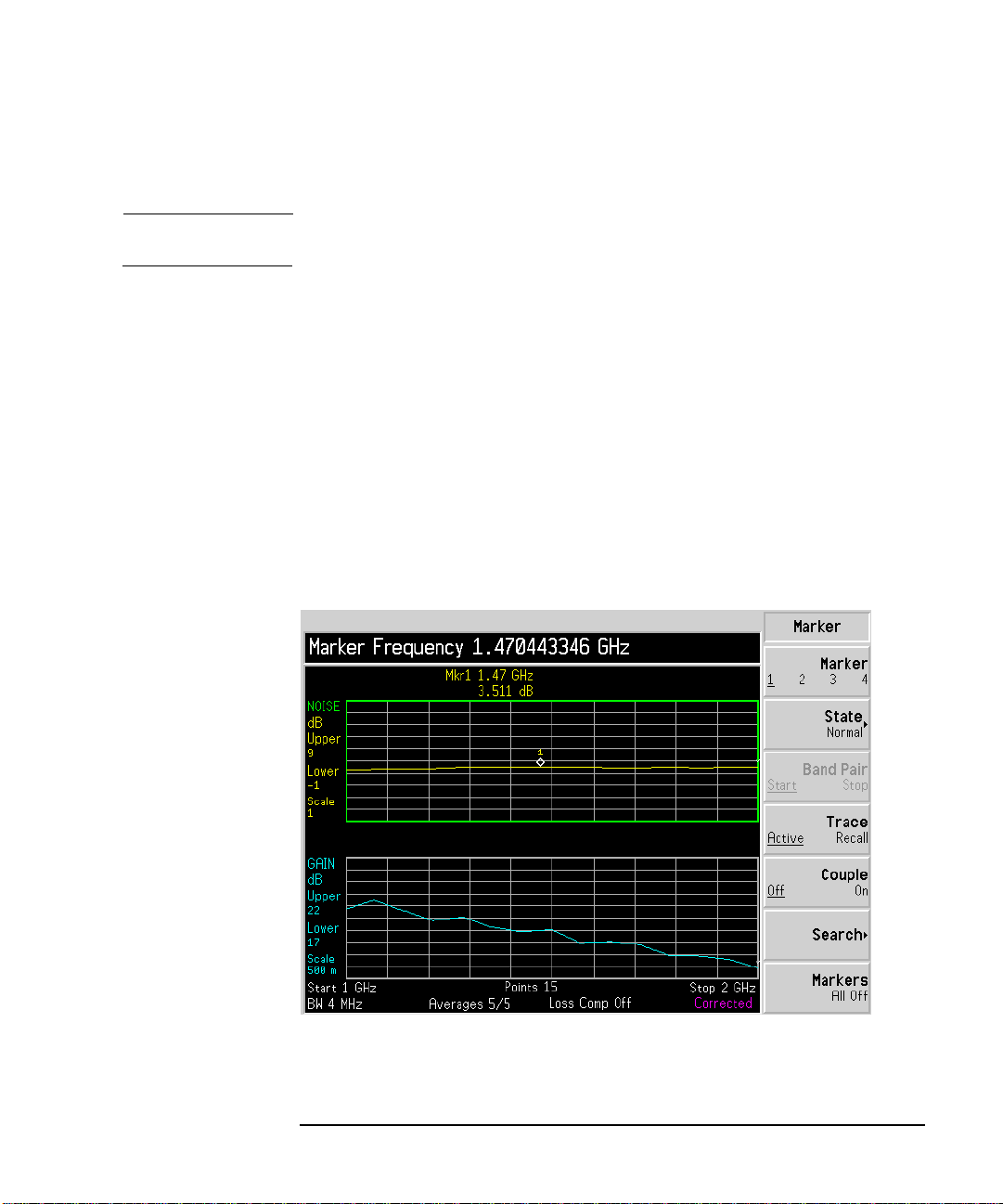
Selecting Markers

To select a marker:

Step 1. Press the Step 2. Press the Step 3. Press the

Marker key.

Marker menu key to select the marker of interest.

State menu key and press the Normal menu key to highlight it.

Figure 2-10 One Marker in Normal State

Turn the RPG to place the marker at the p oint on the trace you want to measure or use the numeric keys to enter the frequency of interest.

Chapter 2 43

Making Basic Measurements

Displaying the Measurement Results

To turn an active marker off

To turn an active marker off press the State menu key and press the Off menu key to highlight it. Thi s also removes the marker annotation from the display and uncouples any marker functions.

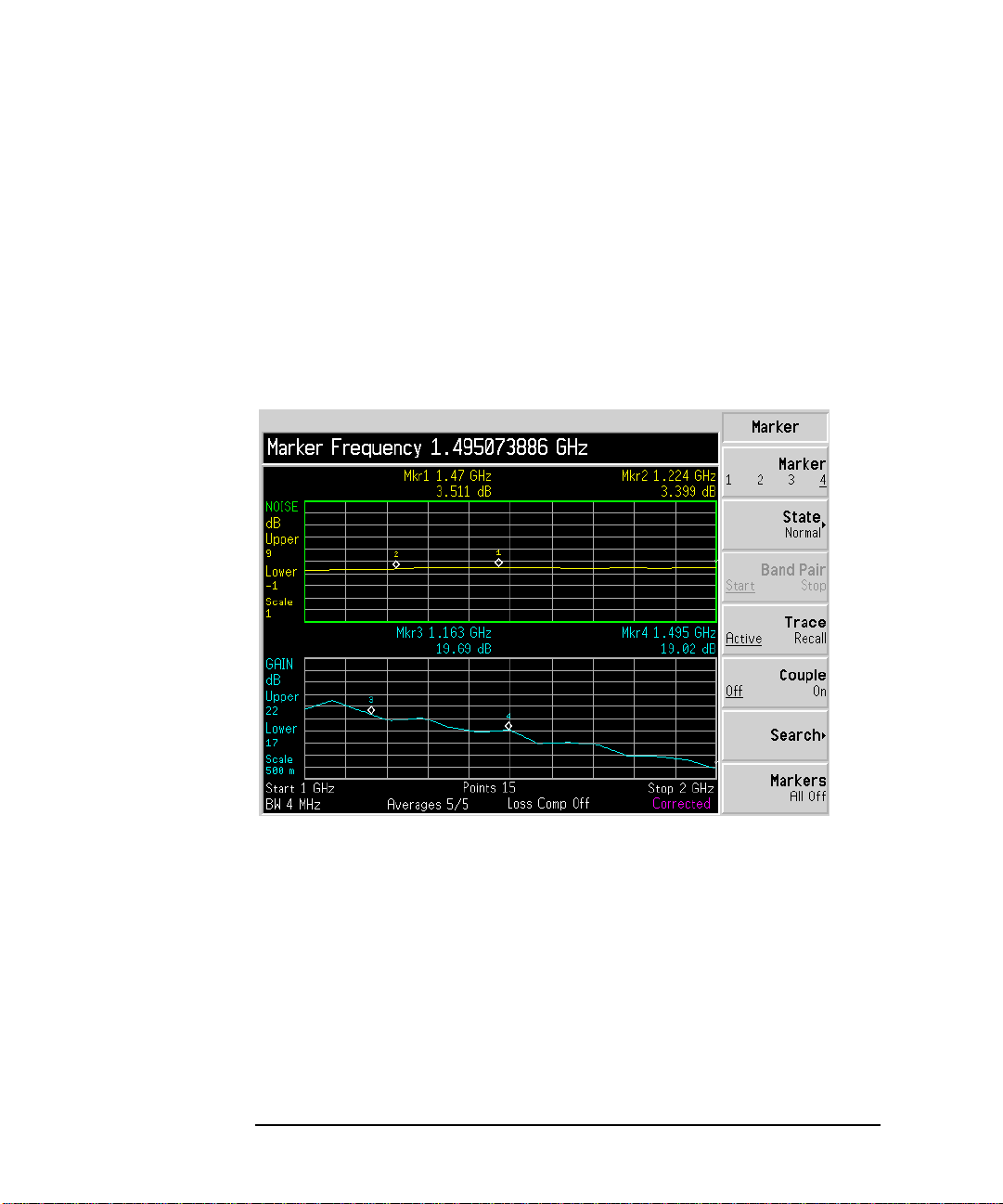
To change the active marker

The default active marker setting is marker, press the

Marker(1⇑ ) to Marker(2⇑ ). Press it again and it moves the active marker

Marker(2⇑ ) to Marker(3⇓).This process is repeated until it returns to

from

Marker(1⇑ ).SeeFigure2-11.

the

Marker menu key. This moves the active marker from

Figure 2-11 Four Markers in Normal State

Marker(1⇑ ). To change the active

To Switch all the Markers Off

To switch all the markers off press

Markers(All Off). This turns off all the

markers and associated annotation.

44 Chapter2

Changing the Marker States

Making Basic Measurements

Displaying the Measurement Results

To use Delta Markers

Step 1. Press the Step 2. Press the Step 3. Press the

To use Band Pair Markers

Step 1. Press the

State(Delta) menu key places a reference marker at the current

The position of the active marker. This enables you to measure the difference

between the reference marker and an active marker position on the trace.

To activate a Delta marker:

Marker key. Marker menu key to select t he marker of interest. State menu key and press the Delta menu key to highlight it.

UsetheRPGtomovetheDeltamarkerfromthereference.The annotation displays the difference.

State(Band Pair) menu key places two markers allowing you t o choose

The to move either the normal marker or the reference marker. The position

of the reference marker remains fixed until

Band Pair(Normal) menu key

is pressed and the active marker becomes the fixed marker. This can be altered by pressing the

Band Pair(Ref) menu key to enable the reference

marker as the active marker. The active marker has its frequency and noise parameter values annotated in the display window relative to the reference marker.

To activate the Band Pair Markers:

Marker key.

Step 2. Press the Step 3. Press the

Marker menu key to select t he marker of interest. State menu key and press the State(Band Pair) menu key to

highlight it.

Step 4. Use the RPG to move the active marker from the reference. The

annotation displays the difference between the reference and the normal markers position.

Chapter 2 45

Making Basic Measurements

Displaying the Measurement Results

Figure 2-12 Band Pair with Normal Marker Enabled

Marking Memory Traces

To place a marker on the recalled memory trace:

Step 1. Enable the

T race(Memory) menu key.

Step 2. Set the marker you want to use to

The marker is placed on the memory trace. If Trace(Data&Memory) is enabled, switching between

Trace(Data) and Trace(Memory) switches the

marker between the traces.

46 Chapter2

Normal, Delta,orBand Pair

Coupling Markers

To couple markers between the upper and lower graph traces:

Step 1. Place a marker on both traces.

For details on setting markers, see “Selecting Markers” on page 43.

Making Basic Measurements

Displaying the Measurement Results

Step 2. Press the

Couple menu key to set the Couple(On) each of the markers.

The markers have their frequency and noise parameter values annotated in the display window.

Figure 2-13 Coupled Markers

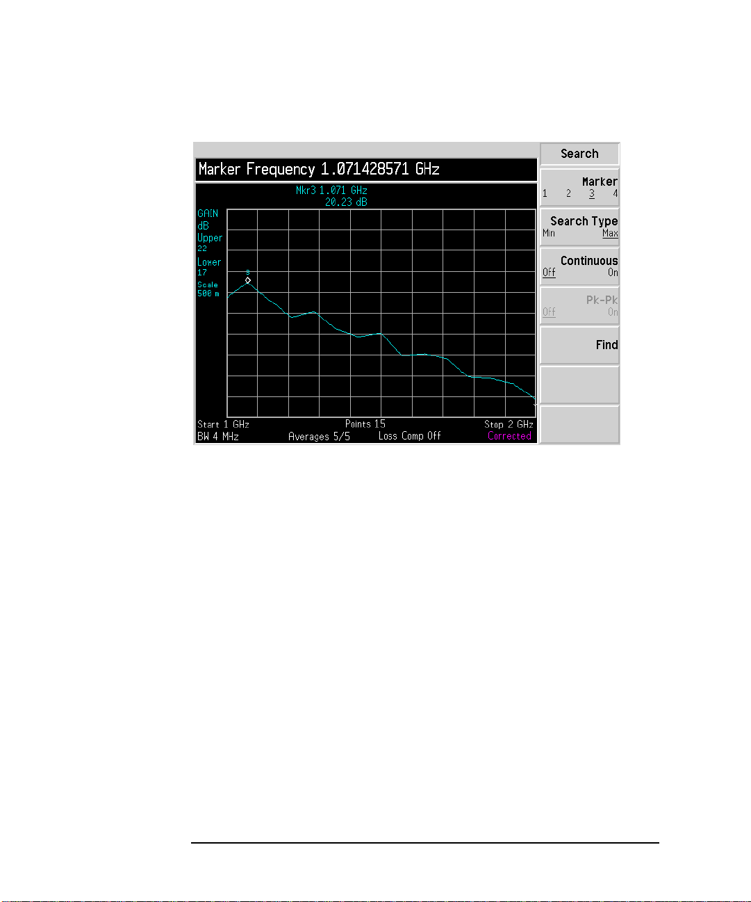
Searching for Min or Max point

Searching with Markers

You need to have activated a marker state to Normal or Delta to perform a minimum or maximum search.

Chapter 2 47

Making Basic Measurements

Displaying the Measurement Results

Figure 2-14 Typical Trace showing Maximum Point Found

Step 1. Press the Step 2. Press the Step 3. Press the

SearchingforPeak to Peak points

To search for the minimum point, select the

Search menu key. Search Type menu key to select the Search Type(Min). Find menu key.

Search Type(Min):

If you want to continuously find the maximum point on the trace, select

Continuous(On).

You need to have activated a marker state to Band Pair to perform a Peak to Peak search.

48 Chapter2

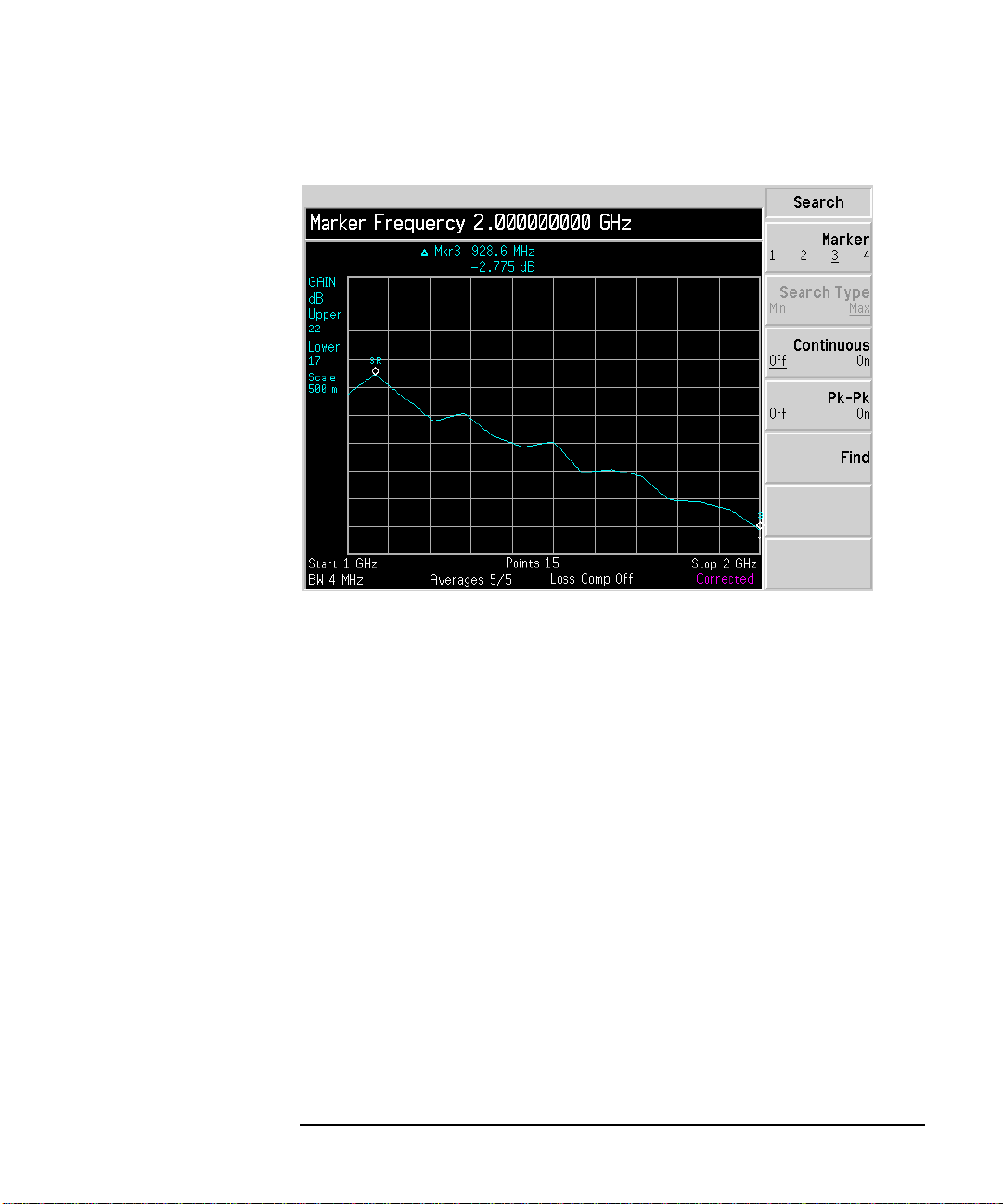
Figure 2-15 Peak to Peak Found

Making Basic Measurements

Displaying the Measurement Results

Step 1. Press the Step 2. Press the Step 3. Press the

If you want to continuously find the maximum and minimum points on the trace, select

Chapter 2 49

Search menu key. Search Type menu key to select Pk-Pk(On). Find menu key.

Continuous(On).

Making Basic Measurements

Indicating an Invalid Result

Several invalid result conditions may exist simultaneously. These conditions are ranked in order of severity and only the most severe condition present is displayed.

The ranking order is:

Table 2-1 Ranking Order of Invalid Result Conditions

Ranking Order Invalid Result Condition Marker Indicator

1 Hot power ≤cold power "==" 2 Corrected calculation not possible "xx" 3 Measurement result calculation

invalid

The ranked condition 2 only occurs if a corrected measurement is requested and either:

• The RF range used at this measurement point is not calibrated.

• The RF range is calibrated, but the calibration data is invalid at this point.

"--"

50 Chapter2

3 Advanced Features

This chapter describes how to use the Limit Lines and Loss Compensation features on your Noise Figure Analyzer.

Advanced Features

WhatYouwillFindinthisChapter

What You will Find in this Chapter

This chapter covers:

• Setting up Limit Lines and using them for pass/fail testing of the measurements.

• Setting Loss Compensation and using this to correct for losses in cabling, switches, or connectors caused by temperature variations etc.

52 Chapter3

Advanced Features

Setting up Limit Lines

The Noise Figure Analyzer features four independent Limit Lines. The

Limit Line(1⇑ ) and Limit Line(2⇑ ) are applied to the upper graph, and Limit Line(3⇓) and Limit Line(4⇓) are associated with the lower graph.

To change the Limit Line

Setting the Type of Limit Line

The default limit line setting is press the

Limit Line(1⇑ ) to Limit Line(2⇑ ), press it again and it moves the active

marker from it returns to the

Limit Line menu key. This moves the active marker from

Limit Line(2⇑ ) to Limit Line(3⇓).This process is repeated until

Limit Line(1⇑ ).

Toset the limit line type, choose trace or

Type(Lower) if you want it to be below the trace. Each of the four

Limit(1⇑ ).Tochangetheactivemarker,

Type(Upper)ifyouwantittobeabovethe

limit line needs to be set up separately.

Enabling Testing against a Limit Line

Toset the testing of the trace against the limit line, choose want to result reported or

Test(Off) if you do not want the result reported.

Each of the four limit line needs to be set up separately.

Test(On) if you

NOTE After a failure the resultant report remains displayed until you switch

Test(Off) or change the limit line type.

To Display a Limit Line

To display the limit line, choose choose

Display(Off). Each of t he four limit line needs to be set up

Display(On). To not display the limit line,

separately.

To Switch all the Limit Lines Off

To switch all the Limit Lines off press simultaneously switches off all Limit Lines regardless of what graph or

Limit Lines(All Off).This

trace they are associated with.

NOTE When a limit line is switched off the limit line data is not affected.

Chapter 3 53

Advanced Features

Setting up Limit Lines

Creating a Limit Line

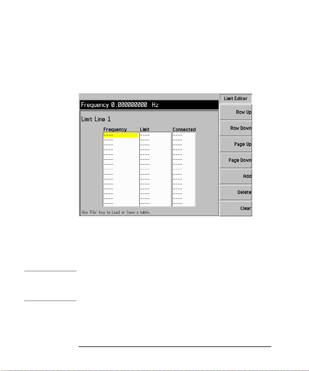
Step 1. Press the Limit Lines key and select the limit line you want to create. Step 2. Press the

Editor menu key.

Figure 3-1 Limit Line Table

Step 3. Enter the first Frequency value. Press the Step 4. Enter the first Y-axis unit value. This value needs to calculated from the

scale you are using to display the trace. Press the

Tab key.

Step 5. Repeat this process until the limit line is defined.

NOTE Connected set to Yes connects the points to form a continous line. To

disconnect any points, set Connected to

No for the points(s) by pressing

the arrow keys.

The limit line is now defined. Press the

Prev key or Limit Line key to

return to the limit line menu. To save a limit line table you save it as a limit line choosing which limit line number you want. See “Saving a File” on page 15.

54 Chapter3

Setting Loss Compensation

You can configure the Noise Figure Analyzer to compensate for losses due to cabling, connectors and temperature effects that occur in t he

measurement s etup between the Noise Source and the DUT, and between the DUT and the Noise Figure Analyzer input.

Configuring Loss Compensation

Step 1. Press the Loss Comp key to access the Loss Compensation form.

Figure 3-2 Loss Compensation Form

Advanced Features

Setting Loss Compensation

Step 2. When configuring loss compensation before the DUT, use the

navigate to the menu key to highlight it.

Step 3. Set the loss compensation value before the DUT, use the

navigate to the the loss occurring before the D UT.

Step 4. Set the temperature value before the DUT, use the

Chapter 3 55

Before DUT fieldandsetittoONbyselectingtheOn

Tab key to

Before DUT Value field and input the required value for

Tab key to navigate to

Tab key to

Advanced Features

Setting Loss Compensation

the Before Temperature field and input the required temperature loss value occurring before the DUT.

Step 5. When configuring loss compensation after the DUT, use the

navigate to the

After DUT fieldandsetittoONbyselectingtheOn menu

key to highlight it).

Step 6. Set t he loss compensation value after the DUT, use the

navigate to the

After DUT Value field and input the required value for the

Tab key to

loss occurring after the DUT.

Step 7. Set the temperature value after the DUT, use the

After Temperature field and input the required temperature loss value

the

Tab key to navigate to

occurring after the DUT.

Tab key to

56 Chapter3

4 Performing System Operations

This chapter describes how to perform the system-level tasks, such as configuring the Noise Figure Analyzer’s GPIB address, defining the preset conditions and configuring an external LO.

Performing System Operations

WhatYouwillFindinthisChapter

What You will Find in this Chapter

This chapter covers:

• Setting the GPIB Addresses

• Configuring the Serial Port

•ConfiguringtheLOGPIB

• Configuring the Characteristics of an External LO

• Configuring the Internal Alignment

• Displaying Error, System and Hardware Information

• Presetting the Noise Figure Analyzer

• Defining the Power-On/Preset Conditions

• Restoring System Defaults

• Setting the Time and Date

• Configuring a Printer

58 Chapter4

Performing System Operations

Setting the GPIB Addresses

NOTE The LO GPIB does not support a Network Analyzer or plotters.

To Set the GPIB Addresses

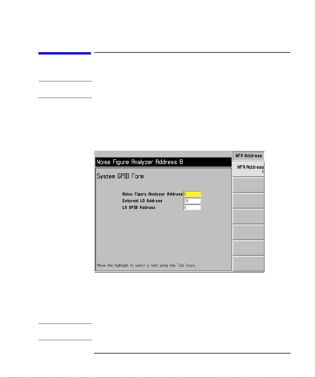
Step 1. Press the System key and press the GPIB menu keys.

Figure 4-1 System GPIB Form

Step 2. Using the

parameters as required. Fora description of the GPIB parameters, see the analyzer online help or

the User’s Guide.

NOTE Ensure the Remote Port menu key is set Remote Port(GPIB).

Chapter 4 59

Tab key to navigate through the form configure the GPIB

Performing System Operations

Configuring the Serial Port

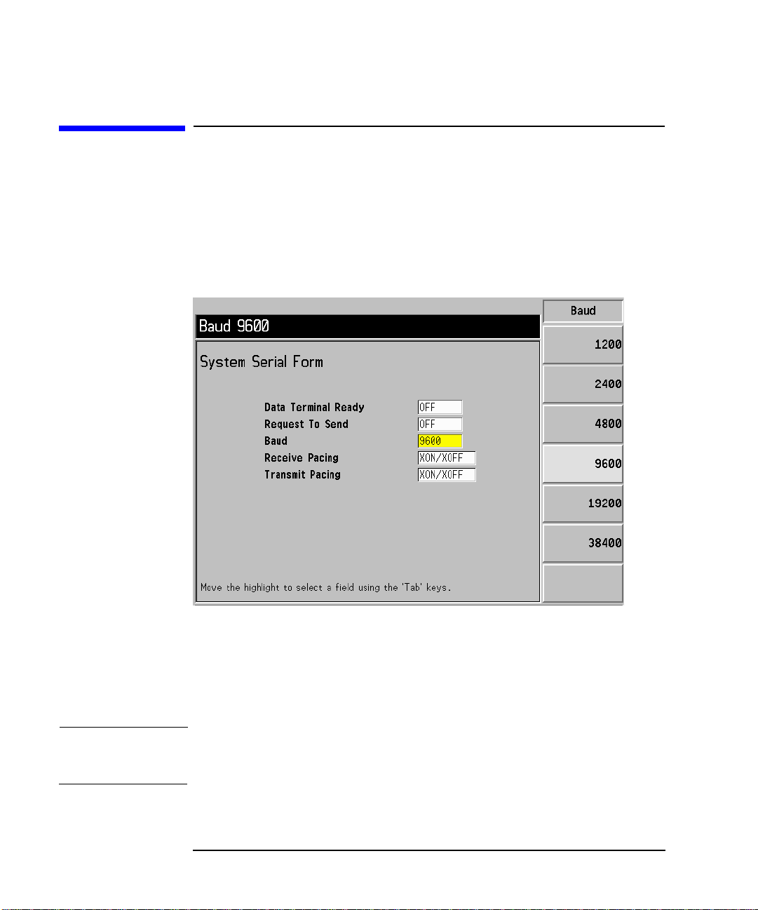
Step 1. Press the System key Step 2. Press the

The System Serial Form now appears. See Figure 4-2

Figure 4-2 System Serial Form

Serial menu key.

Step 3. Use the

configure the serial parameters as requ ired. Fora description of the serial para meters, see the analyzer online help or

the User’s Guide.

NOTE Ensure the Remote Port menu key is set Remote Port(Serial).Thisneedsa

power cycle to take effect.

60 Chapter4

Tab keys to navigate through the form and the menu keys to

Configuring the LO GPIB

Step 1. Press the System key

Performing System Operations

Configuring the LO GPIB

Step 2. Press the

LO GPIB menu key.

YouarepresentedwithaSystem LO GPIB Form.SeeFigure4-3

Figure 4-3 System LO GPIB Form

Setting the LO GPIB Control

This enables or disables the NFA as the LO GPIB controller. When the LO GPIB Control is highlighted, the menu keys for this are

presented to you. To disable the NFA as the LO GPIB controller, set the

LO GPIB(Off). When the NFA is disabled, another instrument on the

GPIB can act as controller. To enable the NFA as the LO GPIB controller, set the

LO GPIB(On).

Chapter 4 61

Performing System Operations

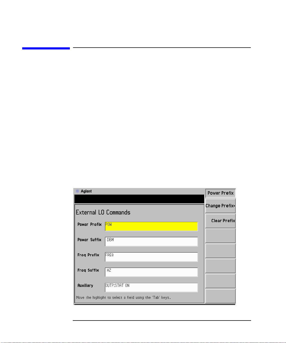
Configuring the Characteristics of an External LO

The NFA can control an external LO using its LO GPIB port.

Custom Command Set

If the LO has a GBIB you are unlikely to use the custom command set. However, you can customize a command set to define the operation of a non-GPIB compatible LO.

To access the menu to configure the command characteristics of an external LO:

Step 1. Press the Step 2. Select the Step 3. Select the

Figure 4-4 External LO Commands Form

System key.

External LO menu key. LO Commands menu key.

62 Chapter4

Performing System Operations

Configuring the Characteristics of an External LO

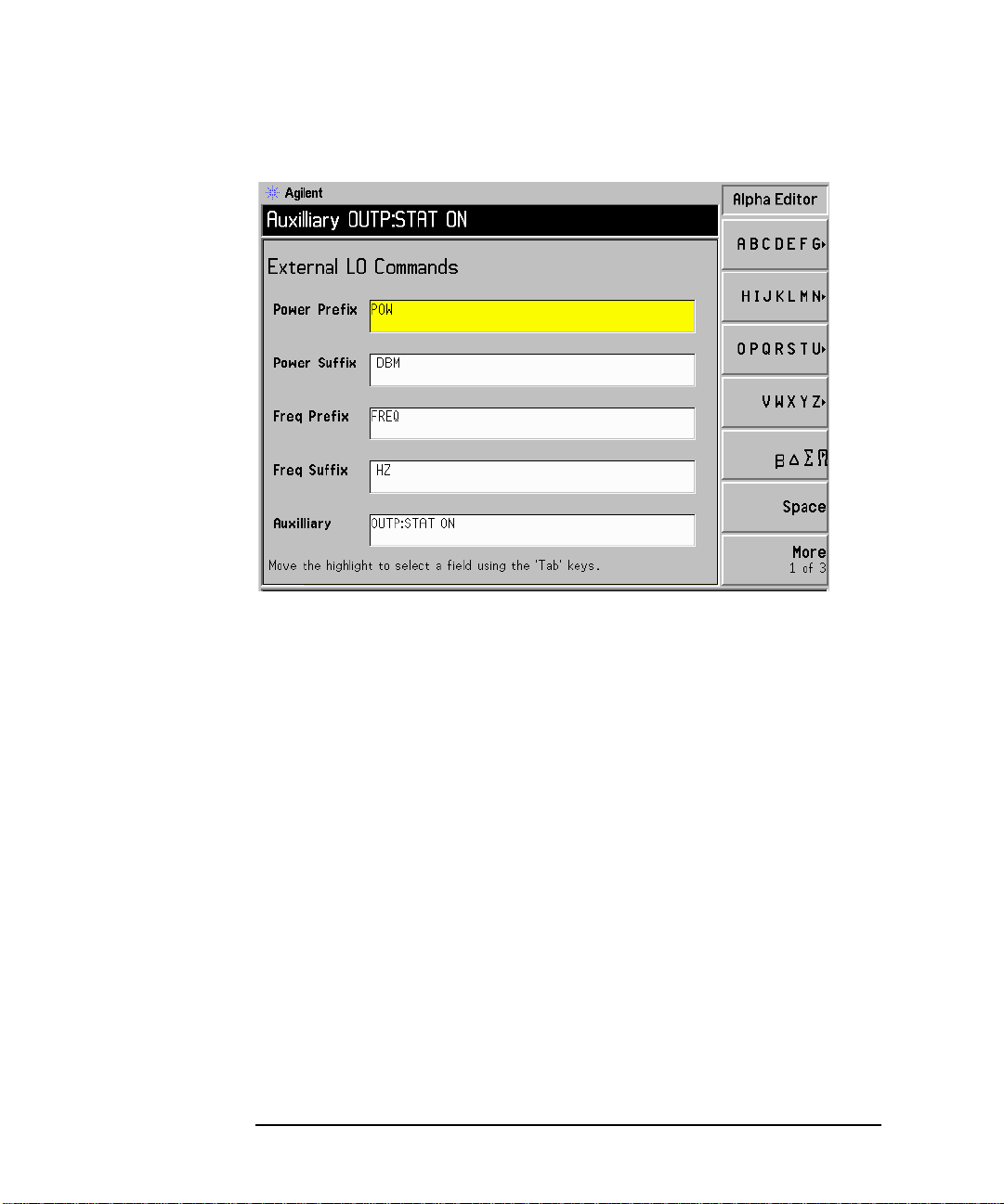
NOTE The default suffix commands have an intentional space inserted.

Step 4. Press the

Tab key to move the highlight to the required position in the

form. You can choose to enter the Prefix and Suffix of the power and frequency.

Also you can enter an auxiliary command. This procedure explains this process using the auxiliary commands.

Figure 4-5 External LO Auxiliary Menu Keys

• Selecting the

Clear Command menu key,clears the current command.

See Figure 4-5 showing the Auxiliary menu keys.

• Selecting the

Change Command menukey,youarepresentedwithan

Alpha Editor,allowingyou to enter a command string using it and the numeric keys, see Figure 4-6. Press the

Prev key to enter the

command. The command string can have up to a maximum of Seventy-nine (79) characters.

Chapter 4 63

Performing System Operations

Configuring the Characteristics of an External LO

Figure 4-6 External LO Auxiliary Command Changes

Settling Time

ThepurposeofthesettlingtimeistoensurethattheNFAwaitsa sufficient amount of time after issuing a command to allow the LO’s

output to stabilize. Pressing the

NFA. Valid settling times are between 0 ms and 100 s. The default value is 100 ms.

64 Chapter4

Settling Time menu key allows you to set the settling time of

Performing System Operations

Configuring the Characteristics of an External LO

Minimum and Maximum Frequencies

The minimum and maximum frequencies, in most cases, represent the frequency capability of the LO. However, they do not affect the LO and

are only used by the NFA to determine if the requested frequency parameter is acceptable. If an attempt to enter an out-of-range frequency is made, the NFA displays an invalid frequency entry error message.

Pressing the the NFA expects the External LO to have. The default value is 10 MHz.

Pressing the frequency the NFA expects the External LO to have. The default value is

26.5 GHz.

Min Freq menu key allows you to set the minimum frequency

Max Freq menu key allows you to set the maximum

Chapter 4 65

Performing System Operations

Configuring the Internal Alignment

Data from the internal alignment routine is necessary for accurate NFA operation and when enabled, the internal alignment routine runs continuously to ensure that the NFA is using current alignment data which improves the NFA’s accuracy.

Turning Alignment Off and On

Step 1. Press the System key. Step 2. Press the Step 3. Press the

Alignment(Off) as required.

The default is alignment on.

Alignment menu key to access the Alignment menu. Alignment menu key to turn alignment Alignment(On) or

Changing Alignment Mode

Step 1. Press the System key. Step 2. Press the Step 3. Press the

Mode(Point)

The default is alignment mode is sweep.

Alignment menu key to access the Alignment menu. Alignment Mode menu key to turn alignment mode Alignment

or Alignment(Sweep) as required.

66 Chapter4

Displaying Error, System and Hardware Information

Displaying the Error History

Step 1. Press the System key.

Performing System Operations

Displaying Error, System and Hardware Information

Step 2. Press

Show Errors menu key to view the error queue.

To clear the error screen, press

Displaying System Information

Step 1. Press the System key. Step 2. Press

Show System menu key to view system information.

Displaying Hardware Information

Step 1. Press the System key. Step 2. Press

Show Hdwr menu key to view hardware information.

Clear Error Queue.

Chapter 4 67

Performing System Operations

Presetting the Noise Figure Analyzer

To preset the analyzer using its factory defaults:

Step 1. Turn the NFA on by pressing the

process to complete.

Step 2. Press Step 3. Press the green

NOTE Turning on the analyzer performs an instrument preset. Turning on the

System, Power On/Preset, Preset (Factory).

Preset key.

analyzer also fetches alignment data; clears both the input and output buffers; turns off limit line testing; and sets the status byte to 0. The last state of the analyzer before it was turned off is recalled when

Power On(Last) is pressed (under the System key).

On key and wait for the power-up

68 Chapter4

Defining the Power-On/Preset Conditions

You can set the NFA so that it returns to a user-defined state upon power-up and preset. The power-up and preset conditions can be

different if required.

Setting the Power On Conditions

Step 1. Press the System front panel key.

Performing System Operations

Step 2. Press the Step 3. Set

Power On/Preset menu key.

Power On to Power On(Last) or Power On(Preset) as required.

‘Last’ means that the instrument, upon power-up returns to th e state it wasinwhenitwaspoweredoff.

‘Preset’ means the instrument returns to its defined preset state.

Setting the Preset Conditions

YoucansettheNFAtoreturntoitsfactorydefaultstateorauser defined state upon preset.

To set the preset conditions to factory default

Step 1. Press the Step 2. Press the Step 3. Enable the

To set the preset conditions to user defined

Step 1. Configure the NFA to the desired state. Step 2. Press the

System front panel key. Power On/Preset menu key.

Preset(Factory) menu key.

System front panel key.

Step 3. Press the Step 4. Enable the Step 5. Press the

Chapter 4 69

Power On/Preset menu key.

Preset(User) menu key.

Save User Preset menu key to save the current NFA state.

Performing System Operations

Restoring System Defaults

Step 1. Press the System key Step 2. Press the

Step 3. Press the

More 1 of 3 menu key. Restore Sys Defaults menu key.

70 Chapter4

Setting the Time and Date

To turn the time and date on and off

Step 1. Press the System key.

Performing System Operations

Setting the Time and Date

Step 2. Press the Step 3. Press the

Time/Date(Off) as required.

Time/Date menu key. Time/Date menu key to turn alignment Time/Date(On) or

To set the time and date

Step 1. Press the System key. Step 2. Press the Step 3. Set the

format (Day/Month/Year).

Step 4. Set the time in hhmmss (hours, minutes seconds) format. Step 5. Set the date in yyyymmdd (year, month, day) format.

Time/Date menu key.

Date Mode to either US format (Month/Day/Year) or European

Chapter 4 71

Performing System Operations

Configuring a Printer

Printer connection Toconnect your printer t urn off the printer and the NFA and connect the

printer to the parallel I/O interface connector of the NFA using an IEEE 1284 compliant parallel printer cable.

If appropriate, configure your printer (see your printer documentation for more details on configuring your printer).

To Configure a Printer

Step 1. Power on the NFA and the printer. Step 2. Press the

to the analyzer online help or User’s Guide for a description of the options.

Step 3. Press

Printer Type to access the Printer Type menu keys and press Auto to

make the NFA attempt to identify the connected printer. The printer should now be automatically recognised by the NFA. If the

printer is not automatically recognised, then see the User’s Guide for more details on printer setup.

Testing Correct Printer Operation

When printer setup is complete test correct printer operation by pressing

Print Setup, Print (Screen) andthenpressingthePrint key to print a test

page.

Print Setup key and then press the Printer Type menu key. Refer

72 Chapter4

Index

Numerics

10 MHz ref in, 7 10 MHz ref out, 7

active function address GPIB alignment, 66 annotation arrow keys AUX IN (TTL), 7 AUX OUT (TTL) Averaging

band pair marker Bandwidth

calibration

performing, 34

configuring

alignment mode loss compensation, 55 serial port

Connector

, 7

GPIB

connector

10 MHz ref in 10 MHz ref out, 7 50 ohm input AUX IN (TTL) AUX OUT (TTL), 7 externalkeyboard LO GBIB noise source output, 5 parallel port probe power RS-232 port, 7 service

CONTROL functions

, 12

, 59

, 8 , 5

, 7

, 33

, 45

, 33

, 34

, 66

, 60

, 7

, 5

, 7

, 5

, 7

, 5

, 4

copy files creating a frequency list custom command, 62

data invalid indicator delete files delta marker, 45 disk format display

combining graph display reference format full screen, 38 memory trace scaling single graph, 39

display annotation DISPLAY functions Displaying

Error History

displaying

hardware information system information

ENR ENR spot value, 28 ENR table cal ENR table common ENR table data entry, 24 ENR table meas entering ENR data Error queue

clearing

Esc key external keyboardconnector, 5 external LO

configuring custom commands, 62 min and max freq settling time

, 17

, 30

, 9

, 18

, 13

, 39 , 42

, 36

, 40

, 41

, 8

, 4

, 67

, 23

, 24

, 67

, 3

, 62

, 65

, 64

file copying, 17 file deleting, 18 file loading file menu functions

copy delete format load, 16 rename save

file renaming, 16 file saving fixed ENR floppy disk format, 13 format format a disk freq mode

fixed list sweep, 29

front-panel overview full screen full span, 29 fuse

GPIB address

setting, 59

GPIB annunciators

hardware information

displaying

help key

input

power INPUT 50W instrument preset

, 16

, 17

, 18

, 13

, 16

, 15

, 15 , 28

, 36

, 13

, 29

, 38

, 7

, 59

, 9

, 67

, 5

, 6

, 5

, 68

, 3

Index 73

Index

intensity

viewing angle

key overview

limit line 1 limit line 2 limit line 3, 53 limit line 4 LO GBIB load files, 16 loss compensation loss compensation configuring

MAIN GPIB Marker 1 Marker 2, 43 Marker 3 Marker 4 marker state

, 45

delta

markers

band pair selecting

, 45

states

marking memory traces, 46 maximum frequency MEASUREMENT functions menu keys, 3 methods of ENR data entry minimum frequency monitor output, 7

next window noise source

model number

, 3

, 12

, 53 , 53

, 53

, 7

, 55

, 7

, 43 , 43

, 43

, 45

, 43

, 65

, 4

, 24

, 65

, 5

, 25

serial number

noise source output

parallel connector power input Power-On conditions

defining

Preset

defining conditions

Preset key, 4 pressing full span printer output printing, parallel

deskjet epson laserjet, 72 paintjet thinkjet

probe power connector, 5

rear panel features rear-panel overview ref level, 42 rename files RPG RS-232 connector, 7

save files saving

ENR table data scaling selecting a fixed freq selecting markers, 43 serial data output serial port

setting up setting

external LO

GPIB address, 59

, 6

, 69

, 68

, 72

, 5

, 15

, 41

, 60

, 16

, 62

, 7

, 24

, 27

, 5

, 7

, 29

, 6

, 7

, 69

, 32

settling time spot ENR SYSTEM functions, 4

Tab Keys tcold data changing temperature correction, 28

using tables

VGA connector video connector, 7 viewing angle

working with tables

zoom

, 5

, 64

, 28

, 5

, 28

, 19

, 7

, 3

, 19

74 Index

Agilent N8972A Quick Reference Guide

Specifications and Main Features

Frequently Asked Questions

User Manual

Quick Reference Guide

May 2000

Safety Notices

The information contained in this documentissubject to change without notice.

This symbol is used to mark the on position of the power line switch.

This symbol is used to mark the standby position of the power line switch.

This symbol indicates that the input power required is AC.

• Operating temperature: 0° Cto+55° C

• Operating humidity: <95% relative

• Altitude: up to 4500 m

Warranty

LIMITATION OF WARRANTY

EXCLUSIVE REMEDIES

http://www.agilent.com/find/nf/

Manufacturer's Declaration

• At Operator Position.

•NormalOperation.

• According to ISO 7779:1988/EN 27779:1991 (Type Test).

Herstellerbeschein igung

• Schalldruckpegel Lp < 70 dB(A).

•AmArbeitsplatz.

• Normaler Betrieb.

• Nach ISO 7779:1988/EN 27779:1991 (Typprüfung).

1 Getting Started

WhatYouwillFindinthisChapter

What You will Find in this Chapter

This chapter covers the following:

• Overview of the Front-Panel

• Overview of the Rear-Panel

• Display Annotation

• Overview of the Front Panel Keys

• Performing Common File Operations

• Working with Tables

Item Description

SYSTEM functions affect the state of the Noise Figure Analyzer.

The green

PROBE POWER provides power for other accessories.

NOISE SOURCE DRIVE OUTPUT +28V PULSED this

Tab Keys are used to move between table input fields, and to

Pressing Zoom key while in graph mode allows you to

active graph. 17 Press the

Item Description

Power input is the input for the AC line-power source.

2 Line Fuse.Thefuseisremovedbytwistingcounterclockwise

label on the rear panel. 3 Service Connector. The service connector is for service use only.

VGA OUTPUT drives an external VGA compatible monitor with

PARALLEL interface parallel port is for printing only.

RS-232 interface supports remote instrument operation.

10 MHz REF IN accepts an external frequency source to provide

10 MHz REF OUT provides a 10 MHz, 0 dBm minimum,

LO GBIB port is for the control of an external LO by the NFA.

MAIN GPIB interface port supports remote instrument operation.

AUX OUT (TTL) it is not currently supported.

AUX IN (TTL) it is not currently supported.

13 Power On Selection selects an instrument power preference.

Display Annotation

Display Annotation

Each item is given a description and where applicable a function key associated with it.

Item Description

2 The time and date display, controlled by the

3 The marker 1 frequency, controlled by the

4 The marker 1 amplitude. 5 The marker 2 frequency, controlled by the

disappears after a complete sweep. 9 The key menu title, this is dependent on which key is selected. 10 The key menu. 11 A non-active menu key. 12 The marker 4 frequency,controlled by the

menu keys. 13 The marker 4 amplitude. 14 The frequency span or stop frequency, controlled by the

by the 17 The number of points, controlled by the

18 The marker 3 frequency, controlled by the Marker(3⇓)and State

menu keys. 19 The marker 3 amplitude. 20 The number of averages, controlled by the

messages. 22 The bandwidth, controlled by the

This is fixed at 4 MHz on the N8972A model. 23 The center frequency or start frequency, controlled by the

24 The lower trace scale, controlled by the

(This is auto-coupled to 25 and 26.) 25 The lower trace lower limit, controlled by the

key. (This is auto-coupled to 24 and 26.) 26 The lower trace upper limit, controlled by the

key. (This is auto-coupled to 24 and 25.) 27 The lower trace result type, controlled by the 28 The upper trace scale, controlled by the

(This is auto-coupled to 29 and 30.) 29 The upper trace lower limit, controlled by the

key. (This is auto-coupled to 28 and 30.) 30 The upper trace upper limit, controlledbythe

key. (This is auto-coupled to 28 and 29.) 31 The upper trace result type, controlled by the