

Page 1
MitoXpress Xtra
Quick Start Guide
Five Step Workflow
Page 2

Table of Contents
1. Plate Reader Setup 3
Find your plate reader download packet 3
Import protocol/template 3
Define the detection mode 3
2. Signal Optimization 4
Plate reader signal optimization 4
Plate preparation 4
Calculations 5
Adjustments for improved signal detection (S:B and signallevel) 6
Confirmation 6
3. Sample Optimization 7
Adherent cell titration plate 7
Suspension cell titration plate 8
Calculations 9
Adjustments for improved O2 consumption (OCR) 10
4. Running the Assay 11
Example control compound treatment (and FCCP optimization) 11
Day before measurement cell plate preparation 12
Control compound preparation 12
Assay plate preparation 12
5. Data Analysis 13
Guideline for applying data analysis tools to raw data 13
Data analysis tool options 13
This Quick Start provides all you need to know from plate
reader setup and signal optimization, to sample and compound
optimizations, as well as routine assay runs and data analysis.
For detailed instructions on product use, please see the
MitoXpress Xtra user manual.
1
Plate reader
setup
2
Signal
optimization
3
Sample
optimization
4
Running
the assay
5
Data
analytics
2
Page 3
1. Plate Reader Setup
Key steps
1.1 Find your plate reader
download packet
1.2 Import protocol/template
1.3 Define the detectionmode
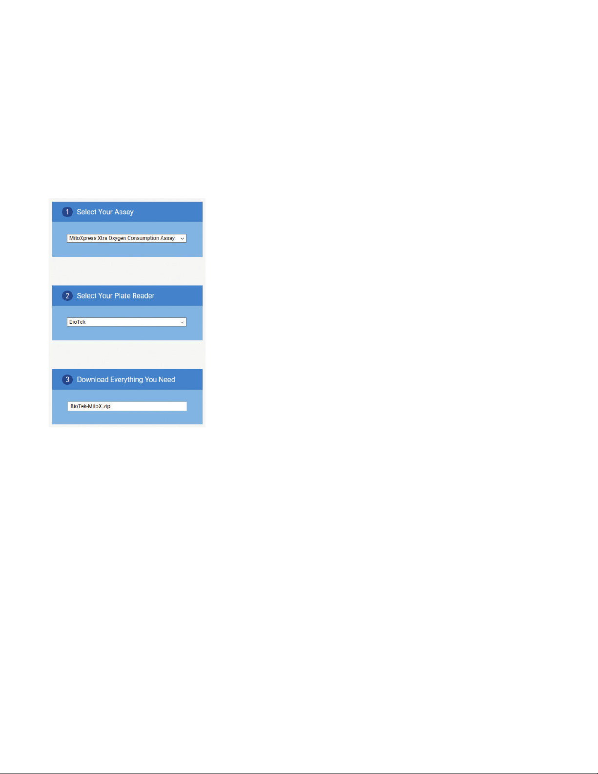
Step 1.1
Find your plate reader download packet
Find your Plate Reader online.
The download packet found in the link above contains the required collateral
and software templates you will need, including the recommended protocol
template files. These files contain default settings for your fluorescence plate
reader model, where available, or an instrument setup guide where not available.
Separately, it will contain a data analysis template specific to your plate reader
control software or, where that is not feasible, provide the data visualization tool
(Excel Macro). In addition, the MitoXpress Xtra user guide is provided, containing
detailed assay instructions.
Step 1.2
Import protocol/template
Import protocol templates into your plate reader software for easy setup. Open
the protocol and define the filter locations specific to your instrument filter
wheel/slide/cube and get started.
If a template is not provided, create a protocol in the instrument software,
inputting the instrument parameters described in the specific instrument
setupguide.
Ensure that software versions are up to date and compatible before starting.
Step 1.3
Define the detection mode
Decide/define which detection mode you intend to employ depending on the plate
reader specification used (basic, standard TR-F, and dual-read TR-F). See the user
guide contained in the download packet to inform your choice.
Use the recommended detection mode for your chosen plate reader
specifications, while ensuring that the correct excitation and emission filters are
installed correctly.
In cases where dual-read TR-F detection is recommended but the filters are not
available, it is possible to employ the standard TR-F detection as an alternative.
This is done using the monochromator rather than filters for excitation and
emission wavelength selection.
3
Page 4

2. Signal Optimization
MX pr
Blank:
Key steps
2.1 Read; 20 minutes at 37°C
2.2 Calculations
i. S:B ratio (>3:1)
ii. Signal level (10 to
20% max. instrument
intensity (RFU))
iii. Lifetime signal level
(22to 26 µs)
2.3 Adjustments
2.4 Confirmation (repeatread)
Step 2.1
Plate reader signal optimization
Measure a cell-free signal optimization plate for verification of the protocol
template/instrument settings implemented in Step 1. This can be done with a
quick assessment of the signal-to-blank (S:B) and signal level (RFU).
• The recommended S:B is >3:1
• The signal level must be ~10 to 20% maximum intensity (RFU) on the plate
reader (~15% of saturation). Otherwise, the signal will overflow/saturate the
instrument.
Usually the default protocol parameters will provide a suitable S:B and RFU;
however, in the unlikely event it is outside these recommendations, simple
adjustments can be made, found in Step 2.3.
Step 2.1.1
Plate preparation
Prepare and read a signal optimization plate using the plate layout in Figure 1.
MitoXpress probe, media, and HS mineral oil preparation are described in the
MitoXpress Xtra user guide.
12345678910 11 12
MX
MX
MX
A
probe
probe
probe
BlankBlank BlankBlank
B
C
D
E
F
G
H
obe: 10 µL MitoXpress probe + 90 µL Media + 100 µL HS mineral oil
100 µL Media + 100 µL HS mineral oil
Figure 1. Signal optimization plate layout.
MX
probe
Note: It is important that the media/sample, HS mineral oil, microplate, and plate
reader are prepared and maintained at the desired assay temperature, 37 °C. The
HS mineral oil should be warmed to 37 °C before the assay for easier use.
4
Page 5
Tip: For consistent, reliable, and quick HS mineral oil dispensing, a repeater
Signal (RFU)
Signal
Blank
type pipette is recommended (using a 1.25 mL syringe tip or 2 mL combitip).
Prepare the repeater syringe tip by trimming ~3 to 4 mm off the tip at a 45°
angle. Remove the internal nozzle from the oil dropper bottle and slowly pick up
the prewarmed HS mineral oil (avoid pipetting up and down, as this can cause
bubbles) and dispense 100 μL into each well at an angle of ~45°, allowing the oil
to flow down the side of each well.
Pipetting tips are found on page 36 of the MitoXpress Xtra user guide.
Key steps
2.1 Read; 20 minutes at 37°C
2.2 Calculations
i. S:B ratio (>3:1)
ii. Signal level (10 to
20% max. instrument
intensity (RFU))
iii. Lifetime signal level
(22to 26 µs)
2.3 Adjustments
2.4 Confirmation (repeatread)
MitoXpress signal
RFU
Step 2.2
Calculations
Perform calculations i. to iii. using one of the following data analysis options:
(a) Plate reader software analysis/templates
(b) Agilent Data Visualization Tool
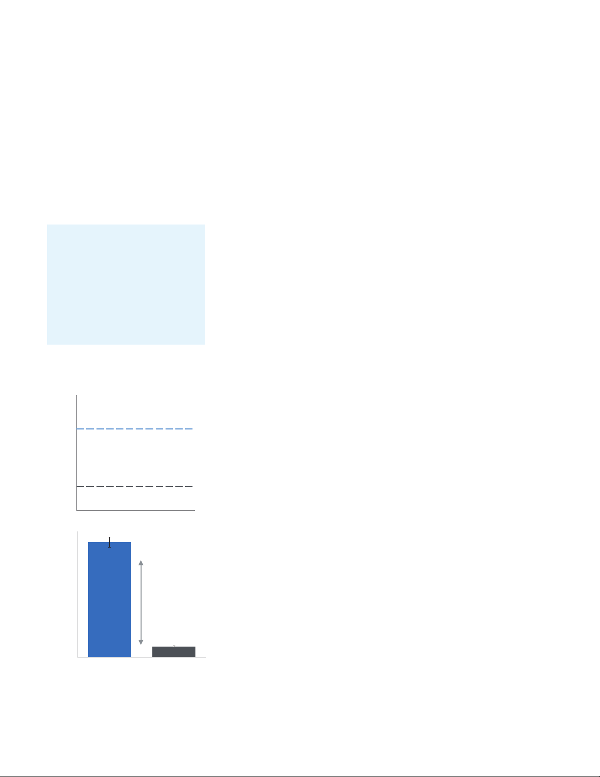
Review the raw results and calculate the following:
i. Signal:blank ratio: Using average RFU values measured at the 20-minute
time point, calculate signal RFU (row A)/blank RFU (row B). Ensure
that the S:B ratio is >3. If using a TRF detection mode: S:B >5 to 10 is
achievable.
ii. RFU signal level: Using RFU signal at the 20-minute time point, the
measured RFU signal level for the MX probe samples should be in the
range of ~10 to 20% of the maximum instrument intensity (RFU). See
the plate reader user manual or software help section to identify the
arbitrary maximum/saturated RFU signal level for the given plate reader
model.
iii. Lifetime signal (µs) level: MitoXpress assay signal (21% O2) ~22 to
26µs.
Blank
Note: This calculation is only applicable when using the advanced dual-read TRF
detection mode on a filter-based plate reader.
Time
3000
Decision point:
• If the recommended S:B ratio, signal level, and lifetime values (where
applicable) are successfully achieved, we recommended proceeding to Step 3.
2500
1000
1500
S:B = 11
1000
500
0
• If, however, the recommended S:B ratio, signal level, or lifetime values are not
achieved, we suggest proceeding to Step 2.3 Adjustments.
5
Page 6

Key steps
Step 2.3
2.1 Read; 20 minutes at 37°C
2.2 Calculations
i. S:B ratio (>3:1)
ii. Signal level (10 to
20% max. instrument
intensity (RFU))
iii. Lifetime signal level
(22to 26 µs)
2.3 Adjustments
2.4 Confirmation (repeatread)
Adjustments for improved signal detection (S:B and
signallevel)
If necessary, based on the calculation in Step 2.2, the following adjustments are
recommended:
i. Parameter review and confirmation
First, review and confirm that all instrument parameters were inputted
correctly and not changed or omitted. See the instrument setup guide,
MitoXpress Xtra user guide, and original template protocol.
ii. Focal (Z-) height optimization
To improve RFU signal level and S:B for a given microplate format
and volume, check and adjust the focal height setting manually or
automatically depending on reader capability. See the plate reader user
manual. Only applicable where focal height adjustment is available.
iii. Gain or photomultiplier tube (PMT) setting adjustments
The protocol templates employ fixed gain or PMT settings throughout
the kinetic measurement. Auto Gain, Dynamic, or Variable Gain should
not be used.
• If signal level is too high (>20% max. intensity), decreasing the gain or
PMT setting is recommended.
• If signal level is too low (<10% max. intensity), increasing the gain or
PMT setting is recommended.
Note: If using advanced dual-read TRF detection mode, attention should be on
the RFU signal measured from Window 1 (W1), (30 µs delay read/window), when
targeting 10 to 20% max. intensity. Also, both W1 and W2 TRF settings must
use identical gain settings; this is critically important to a successful lifetime
signal-based assay.
iv. Flash number, or number of pulses
Increase the flash number (no.) value to yield improved signal stability.
Highest flash no. will yield longer cycle time.
Note: Default TRF (time-resolved fluorescence) settings (delay time and
integration/window times) should not be adjusted.
Additional adjustments: Details on these can be found in the Troubleshooting
section of the MitoXpress Xtra user guide. These include switching to bottom
read detection, removal of phenol red and serum from media, or increasing
MitoXpress probe concentration by 5 µL/well, or a combination of all options.
Step 2.4
Confirmation
Repeat Step 2.1 and 2.2 using the same signal optimization plate to verify the
success of any adjustments made in Step 2.3. Once confirmed, move to Step 3.
6
Page 7

3. Sample Optimization
40
Cell titration
120
Slope(µs/h)
Key steps
3.1 Adherent cell titration
Determine the relative oxygen consumption rate (OCR) from a range of cell
densities. Thisis essential for identifying the suitable seeding density required
for detectable metabolism (relative OCR) for a given cell type/model under fixed
3.2 Suspension cell titration
3.3 Calculations
conditions. The cell density required is cell type-specific; these concentrations are
general guidanceonly.
3.4 Adjustments
Step 3.1
80K
60K
36
40K
30K
No cells
32
28
Mitoexpress signal (µs)
24
20
0306090
7.0
6.0
5.0
4.0
3.0
2.0
1.0
0.0
Time (min)
80K
60K
40K
30K
No cells
Adherent cell titration plate
3.1.1 Day before measurement
Plate cells with the following seeding densities: 30,000, 40,000, 60,000, and
80,000/200 µL media overnight (n = 4) using a suitable TC+ 96-well microplate.
The suggested plate layout is provided in Figure 2.
12345678910 11 12
80K 80K 80K 80K
A
60K 60K 60K 60K
B
40K 40K 40K 40K
C
30K 30K 30K 30K
D
0K
E
Signal
F
control
BBllaannkkBBllaannkkBBllaannkkBBllaannkk
G
H
Cell plating densities (X *1000 cells/well): 60K is 60,000 cells/well
Signal control: Media + MitoXpress probe + HS mineral oil
Blank: Media + HS mineral oil
0K 0K 0K
Signal
control
Signal
control
Signal
control
Figure 2. Adherent cell plate layout.
* Optional: Positive signal control (GOx) can be added to row H (n = 4). For example, GOx plus
MitoXpress in media, plus HS mineral oil (positive signal control). *Add 10 µL of 1.5 mg/mL Gox
stock /well. (GOx well concentration: 0.15mg/mL).
Tip: Allow the plate to rest on the bench for 30 minutes at room temperature
after the cells have been pipetted onto the plate. This will help ensure an evenly
dispersed monolayer to help minimize plate edge effects.
7
Page 8

3.1.2 Day of measurement
28
090
Cell titration
Slope(µs/h)
Prepare the cell assay plate as per user manual guidelines, including the
appropriate control and blank samples.
• See the previous recommendation (page 4) to use a repeater type pipette for
optimum HS mineral oil addition.
• Measure the cell titration plate kinetically at 37 °C for two hours using
minimum cycle or interval time (one minute), immediately after the HS mineral
oil layer is applied.
Note: Blank and signal control samples are always required (minimum n = 2) and
should be included in all routine MitoXpress Xtra assays.
Key steps
3.1 Adherent cell titration
3.2 Suspension cell titration
3.3 Calculations
Step 3.2
Suspension cell titration plate
3.2.1 Day of measurement
Plate cells with the following density; 200,000, 300,000, 400,000, and
600,000/90µL media (n = 4) using a suitable 96-well microplate. See Figure 3.
3.4 Adjustments
12345678910 11 12
600K
400K
26
24
22
Mitoexpress signal (µs)
20
7.0
6.0
5.0
4.0
3.0
2.0
1.0
300K
200K
No cells
0306
Time (min)
600K
400K
300K
200K
No Cells
Cell plating densities (X *1000 cells/well): 400K is 400,000 cells/100 µL
Signal control: Media + MitoXpress probe + HS mineral oil
Blank: Media + HS mineral oil
Figure 3. Suspension cell plate layout.
*Optional: Positive signal control (GOx) can be added to row C (n = 4). For example, GOx plus
MitoXpress in media, plus HS mineral oil. Add 10 µL of 1.5 mg/mL GOx stock/well. (GOx well
concentration: 0.15 mg/mL).
600K 600K 600K 600K
A
400K 400K 400K 400K
B
300K 300K 300K 300K
C
200K 200K 200K 200K
D
0K
E
Signal
F
control
BBllaannkkBBllaannkkBBllaannkkBBllaannkk
G
H
0K 0K 0K
Signal
control
Signal
control
Signal
control
0.0
Tip: Temperature control and temperature equilibration of the microplate and
cell suspension during plate preparation is important in minimizing inconsistent
temperature across the plate. Use a plate heat block set to 37 °C where possible.
3.2.2
Prepare the cell assay plate as per the MitoXpress Xtra user guide instructions,
by adding 10 µL MitoXpress/well, including the appropriate control and
blanksamples.
8
Page 9

18,000
Time (min)
09
Mitoexpress signal (RFU)
Key steps
Step 3.3
3.1 Adherent cell titration
3.2 Suspension cell titration
3.3 Calculations
3.4 Adjustments
80K
60K
16,000
14,000
12,000
10,000
8,000
40K
30K
No cells
0306
0
Calculations
Perform these calculations to identify a suitable cell density for use in routine
assays. A suitable cell density is one that yields either of the criteria in i and ii.
Cell density criteria:
i. A signal fold increase (RFU increase) of ~1.3 to 2-fold over a 60-minute
period
ii. A MitoXpress Xtra lifetime signal slope of >4 µs/h if using advanced
dual-read TRF detection mode
If a higher minimum level of signal change (O2 consumption) was preferred, an
even greater cell density could be chosen.
Apply data analysis using one of the options provided:
(a) Plate reader software analysis/templates
(b) Agilent Data Visualization Tool
For more detail, see Step 5 for data analysis recommendations.
3.3.1
To accurately measure slope (signal increase), choose a suitable time range
over which the RFU signal is analyzed. When using the data visualization tool,
visualize the kinetic signal profiles in the chart and choose an appropriate start
time and end time for slope calculation that best captures the linear portion of
the signal profiles from all samples. Typically, this would be after any initial RFU
signal decrease (temperature equilibration of the sample) during the initial 10 to
20minutes.
3.3.2
Review the results and determine the measured rates (slope of signal increase)
of all the titrated samples. Calculate average and standard deviation, and plot
average slope values versus cell density, including the probe-only signal control.
3.3.3
Determine the cell density that achieves the signal fold increase or lifetime
signal slope criteria above.
Decision point:
• If the recommended cell density criteria are successfully achieved, we
recommended proceeding to Step 4.
• If the criteria are not achieved, we recommend performing the adjustments
described in Step 3.4
9
Page 10

Key steps
Step 3.4
3.1 Adherent cell titration
3.2 Suspension cell titration
3.3 Calculations
3.4 Adjustments
Adjustments for improved O2 consumption (OCR)
This is essential for identifying the suitable cell density required for detectable
metabolism (relative OCR) in each cell type/model under fixed conditions. The
cell density required is cell type-specific.
If the cell density criteria are not achieved, we recommend performing some or a
combination of the following adjustments:
i. Re-evaluate the results, ensuring that the correct time range is being
used for analysis (avoid temperature equilibration) and that there
are no outliers, incorrect calculations, or data corrections being
appliedincorrectly.
ii. Repeat the titration experiment, ensuring the following:
• Better temperature control at 37 °C of the media, assay test
plate, plate reader microplate chamber, and HS mineral oil during
platepreparation.
• Accurate control of media and sample volume.
iii. Repeat the titration experiment with an increased cell density (amount
of sample), repeating Step 3 again.
iv. Repeat the titration experiment with a decreased well volume, 75 or
50µL. (for example: 50 µL/well, 10 µL MitoXpress plus 40 µL media). Do
not decrease well volume below 50 µL/well (96-well microplate). The
volume of HS mineral oil added does not change.
After any adjustments/repeat titration experiments, perform Step 3 calculations
again to ensure that cell density criteria are achieved. Only once this is done
should you proceed to Step 4.
10
Page 11

4. Running the Assay
Key steps
4.1 Control compound acute
treatment
4.1.1 Cell plate preparation
4.1.2 Control compound
preparation
4.1.3 Assay plate preparation
and compound addition
Step 4.1
Example control compound treatment (and FCCP optimization)
Prepare a control compound plate as follows:
i. Seed the plate with the optimum cell density (X) identified in Step 3.
ii. Prepare and add control compound treatments described in Step 4.1.2
and in Figure 4.
12345678910 11 12
FCCP
FCCP
FCCP
FCCP
FCCP
FCCP
1 µM
mycin
DMSO
Signal
FCCP
2.5 µM
FCCP
1.25 µM
FCCP
0.625 µM
FCCP
0.313 µM
1 µM
Rot/Anti
mycin
DMSO
control
Signal
control
A
2.5 µM
2.5 µM
FCCP
B
C
D
E
F
G
H
1.25 µM
0.625 µM
0.313 µM
Rot/Anti
control
control
FCCP
1.25 µM
FCCP
FCCP
0.625 µM
FCCP
FCCP
0.313 µM
1 µM
1 µM
Rot/Anti
mycin
mycin
DMSO
DMSO
control
Signal
Signal
control
Blank Blank Blank Blank
2.5 µM
1.25 µM
0.625 µM
0.313 µM
Rot/Anti
control
control
Cell Plating Density: Rows A to F, columns 1 to 4 (for example, adherent cell type: 50,000/well)
FCCP: A range of concentrations from 0.3 µM to 2.5 µM
Rot/Antimycin: 1 µM final concentration
Signal Control: Media + MitoXpress probe + HS mineral oil
Blank: Media + HS mineral oil
Figure 4. Cell compound treatment plate layout. For suspension cell type, plate the cells on the day
of measurement, for example 400,000/100 µL.
*Optional: Positive signal control (GOx) can be added to G3 and G4 wells (n = 2). For example, GOx
plus MitoXpress in media, plus HS mineral oil. Add 10 µL of 1.5 mg/mL GOx stock/well. (GOx well
concentration: 0.15 mg/mL).
11
Page 12

150
MitoXpress Signal (µs)
An
Key steps
Step 4.1.1
4.1 Control compound acute
treatment
4.1.1 Cell plate preparation
4.1.2 Control compound
preparation
4.1.3 Assay plate preparation
and compound addition
A
40
35
30
25
20
B
FCCP
Vehicle
Antimycin A
050 100
Time (min)
20
Day before measurement cell plate preparation
Plate cells with the optimum cell density:
Adherent cells
Plate cells at X *1000 cells/200 µL media overnight (n = 36), using a suitable
TC+96-well microplate. For example, 50,000 cells/200 µL for HepG2 cells row
AtoF, column 1 to 4 of microplate. See Figure 4.
Tip: Allow the plate to rest on the bench for 30 minutes at room temperature,
asbefore.
Suspensions cells
Prepare on the day of measurement as described in Figure 4, rows A throughF,
columns 1 through 4 of the microplate. For example, 400,000 cells/100 µL for
HL60 cells rows A to F, columns 1 to 4 of microplate.
Tip: Prepare a master mix stock of suspension cells in media plus the MitoXpress
Xtra probe, for best consistency.
Step 4.1.2
Control compound preparation
Prepare 100X stock concentrations in vehicle (DMSO):
• FCCP (positive control). A serial 1:2 dilution dose response is advisable
between 2.5 and 0.3 µM, final concentration.
15
10
MitoXpress rate (µs/h)
• Rotenone/Antimycin is the recommended negative control. 1 µM final
concentration.
Note: The information in 4.1.1 and 4.1.2 is general guidance only. Response may
be cell-type dependent. Adjust compound concentrations as required.
Tip: For initial investigative experiments with compounds, measuring at 37 °C
with minimum interval time (one minute) is recommended for a minimum of
5
0
Vehicle
FCCP
timycin A
twohours.
Step 4.1.3
Assay plate preparation
Prepare the assay plate per the user manual instructions, including the
appropriate signal control and blank samples. Adding 1 µL of the control
compounds (100X) stock to the appropriate wells (see Figure 4). Then add
100µL of HS mineral oil (warmed to 37 °C) to all test wells, before starting assay
measurement.
Tip: Prepare a master mix of MitoXpress Xtra probe plus media for the consistent
and simplified addition of MitoXpress reagent. Prepare suitable volume and
excess to dispense 100 µL/well.
For consistent, reliable, and quick HS mineral oil dispensing, see pipetting tips
found in the user manual on page 36.
12
Page 13

5. Data Analysis
Key steps
5.1 Apply data analysis, and
select a suitable time
range for slope analysis
5.2 Data analysis tool options
available:
a) Plate reader software
analytics templates
b) Agilent Data
Visualization Tool
Step 5.1
Guideline for applying data analysis tools to raw data
Using either (a) plate reader software analysis/templates or (b) the Agilent Data
Visualization Tool, all of which are contained in the download packet retrieved in
Step 1, or here:
a) Find your Plate Reader
b) Agilent Data Visualization Tool
To accurately measure slope (signal increase), choose a suitable time range over
which the RFU signal is analyzed. When using the data visualization tool, visualize
the kinetic signal profile chart and choose an appropriate start and end time
for slope calculation that best captures the linear portion of the signal profiles
from all samples. Typically, this should be after any initial RFU signal decrease
(temperature equilibration of the sample) during the initial 10 to 20 minutes.
For plate reader software templates, there are specific functions/buttons for
correctly choosing start and end times for the slope calculations. Look for these
in the slope or the V max reduction/calculation step in each case, and consult the
vendor analysis software user manual if necessary.
Step 5.2
Data analysis tool options
Plate reader software analytics templates
Plate reader software analysis templates or data analysis as part of software
protocol files are available from the following plate reader vendors:
1. BioTek - Gen5 protocols (.prt)
2. BMG Labtech - MARS data analysis templates (.MTF)
3. Molecular Devices - SoftMaxPro protocols (.spr)
Agilent MitoXpress and pH Xtra data visualization tool
Carefully read to the Data Visualization Tool (DVT) user manual before use. Save
and export the results in the designated compatible format, (csv,.txt file) from the
plate reader software.
The data visualization tool is a Microsoft Excel Macro that automatically
transforms experimentally derived fluorescence data into kinetic signal curves,
applies time range slope calculation, with slope and endpoint results conveniently
tabulated and illustrated as charts.
Simple approach
• Export results into the correct DVT-compatible file format: .TXT or .CSV.
• Load the .TXT or .CSV file into DVT.
• Follow the directions for annotation, data visualization, and time range
selection (slope calculation) in the Graph tab.
• Summary data table and charts output available.
13
Page 14

For Research Use Only. Not for use in diagnostic procedures.
DE.404837963
This information is subject to change without notice.
© Agilent Technologies, Inc. 2020
Published in the USA, May 5, 2020
5994-1822EN
 Loading...