Agilent E5071B Programmer's Guide

Download

Agilent E5070B/E5071B ENA Series RF Network Analyzers

Programmer’s Guide

Ninth Edition

FIRMWARE REVISIONS

This manual applies directly to instruments that have the firmware revision A.08.10.

For additional information about firmware revisions, see Appendix A.

Manufacturing No. E5070-90412

June 2007

Notices

The information contained in this document is subject to change without notice. This document contains proprietary information that is protected by copyright. All rights

are reserved. No part of this document may be photocopied, reproduced, or translated to another language without the prior written consent of Agilent Technologies.

Microsoft®,MS-DOS®,Windows®,Visual C++®,Visual Basic®,VBA® and Excel® are registered

UNIX is a registered trademark in U.S. and other countries, licensed exclusively through X/Open Company Limited.

Manual Printing History

The manual’s printing date and part number indicate its current edition. The printing date changes when a new edition is printed. (Minor corrections and updates that are incorporated at reprint do not cause the date to change.) The manual part number changes when extensive technical changes are incorporated.

August 2002 First Edition (part number: E5070-90032) March 2003 Second Edition (part number: E5070-90042, changes for firmware

version A.03.50)

January 2004 Third Edition (part number: E5070-90052, changes for firmware

version A.03.60)

August 2004 Fourth Edition (part number: E5070-90062, changes for firmware

version A.04.00)

May 2005 Fifth Edition (part number: E5070-90072, changes for firmware

version A.05.00)

November 2005 Sixth Edition (part number: E5070-90082, changes for firmware

version A.06.00)

May 2006 Seventh Edition (part number: E5070-90092, changes for firmware

version A.06.50)

February 2007 Eighth Edition (part number: E5070-90402, changes for firmware

version A.08.00)

June 2007 Ninth Edition (part number: E5070-90412, changes for firmware

version A.08.10)

Typeface Conventions

Bold Boldface type is used when a term is defined. For

example: icons are symbols.

Italic Italic type is used for emphasis and for titles of

manuals and other publications.

[Key] Indicates the hardkey whose key label is Key. [Key] - Item Indicates a series of key operations in which you

press the called key and so on, and then press the

[Key] key, select (highlight) the item

Item on the displayed menu using the [↓]

[Enter] key.

Sample Program Disk

A sample program disk (Agilent part number: E5070-180x0) is furnished with this manual. The disk contains the sample programs used in this manual.

The customer shall have the personal, non-transferable rights to use, copy, or modify SAMPLE PROGRAMS in this manual for the customer’s internal operations. The customer shall use the SAMPLE PROGRAMS solely and exclusively for their own purposes and shall not license, lease, market, or distribute the SAMPLE PROGRAMS or modification of any part thereof.

Agilent Technologies shall not be liable for the quality, performance, or behavior of the SAMPLE PROGRAMS. Agilent Technologies especially disclaims any responsibility for the operation of the SAMPLE PROGRAMS to be uninterrupted or error-free. The SAMPLE PROGRAMS are provided AS IS.

AGILENT TECHNOLOGIES DISCLAIMS ANY IMPLIED WARRANTY OF MERCHANTABILITY AND FITNESS FOR A PARTICULAR PURPOSE.

Agilent Technologies shall not be liable for any infringement of any patent, trademark, copyright, or other proprietary right by the SAMPLE PROGRAMS or their use. Agilent Technologies does not warrant that the SAMPLE PROGRAMS are free from infringements of such rights of third parties. However, Agilent Technologies will not knowingly infringe or deliver software that infringes the patent, trademark, copyright, or other proprietary right of a third party.

E5070B/E5071B Documentation Map

The following manuals are available for the E5070B/E5071B.

• User’s Guide (Part Number: E5070-904x0, attached to optional ABA)

This manual describes most of the basic information necessary to use the E5070B/E5071B. It provides a function overview, detailed operation procedure for each function (from preparation for measurement to analysis of measurement results), measurement examples, specifications, and supplemental information. For programming guidance on performing automatic measurement with the E5070B/E5071B, please see the Programming Manual.

• Installation and Quick Start Guide (Part Number: E5070-900x1, attached to

optional ABA)

This manual describes installation after it is delivered and the basic operation procedures for applications and analysis. Refer to this manual when you use the E5070B/E5071B for the first time.

• Programmer’s Guide (Part Number: E5070-900x2, attached to optional ABA)

This manual provides programming information for performing automatic measurement with the E5070B/E5071B. It includes an outline of remote control, procedures for detecting measurement start (trigger) and end (sweep end), application programming examples, command reference, and related informatio n.

• VBA Programmer’s Guide (Part Number: E5070-900x3, attached to optional ABA)

This manual describes programming information for performing automatic measurement with internal controller. It includes an outline of VBA programming, some sample programming examples, a COM object reference, and related information.

NOTE The number position shown by “x” in the part numbers above indicates the edition number.

This convention is applied to each manual, CD-ROM (for manuals), and sample programs disk issued.

1. Making Effective Use of This Manual

Contents of This Manual. . . . . . . . . . . . . . . . . . . . . . . . . . . . . . . . . . . . . . . . . . . . . . . . . . . . . . . . . . . . . . . . 24

How To Use This Manual. . . . . . . . . . . . . . . . . . . . . . . . . . . . . . . . . . . . . . . . . . . . . . . . . . . . . . . . . . . . . . . 26

Looking up SCPI commands. . . . . . . . . . . . . . . . . . . . . . . . . . . . . . . . . . . . . . . . . . . . . . . . . . . . . . . . . . . 26

Using sample programs. . . . . . . . . . . . . . . . . . . . . . . . . . . . . . . . . . . . . . . . . . . . . . . . . . . . . . . . . . . . . . . 27

2. Overview of Remote Control

Types of remote control system . . . . . . . . . . . . . . . . . . . . . . . . . . . . . . . . . . . . . . . . . . . . . . . . . . . . . . . . . . 30

GPIB remote control system . . . . . . . . . . . . . . . . . . . . . . . . . . . . . . . . . . . . . . . . . . . . . . . . . . . . . . . . . . . . 31

What is GPIB? . . . . . . . . . . . . . . . . . . . . . . . . . . . . . . . . . . . . . . . . . . . . . . . . . . . . . . . . . . . . . . . . . . . . . 31

System configuration . . . . . . . . . . . . . . . . . . . . . . . . . . . . . . . . . . . . . . . . . . . . . . . . . . . . . . . . . . . . . . . . 31

Device selector . . . . . . . . . . . . . . . . . . . . . . . . . . . . . . . . . . . . . . . . . . . . . . . . . . . . . . . . . . . . . . . . . . . . . 32

LAN remote control system . . . . . . . . . . . . . . . . . . . . . . . . . . . . . . . . . . . . . . . . . . . . . . . . . . . . . . . . . . . . . 33

System configuration . . . . . . . . . . . . . . . . . . . . . . . . . . . . . . . . . . . . . . . . . . . . . . . . . . . . . . . . . . . . . . . . 33

Control over SICL-LAN server. . . . . . . . . . . . . . . . . . . . . . . . . . . . . . . . . . . . . . . . . . . . . . . . . . . . . . . . . 34

Control over telnet server . . . . . . . . . . . . . . . . . . . . . . . . . . . . . . . . . . . . . . . . . . . . . . . . . . . . . . . . . . . . . 39

USB Remote Control System . . . . . . . . . . . . . . . . . . . . . . . . . . . . . . . . . . . . . . . . . . . . . . . . . . . . . . . . . . . . 42

System configuration. . . . . . . . . . . . . . . . . . . . . . . . . . . . . . . . . . . . . . . . . . . . . . . . . . . . . . . . . . . . . . . . . 42

Sending SCPI command messages . . . . . . . . . . . . . . . . . . . . . . . . . . . . . . . . . . . . . . . . . . . . . . . . . . . . . . . 48

Types and structure of commands . . . . . . . . . . . . . . . . . . . . . . . . . . . . . . . . . . . . . . . . . . . . . . . . . . . . . . 48

Grammar of messages . . . . . . . . . . . . . . . . . . . . . . . . . . . . . . . . . . . . . . . . . . . . . . . . . . . . . . . . . . . . . . . 49

Remote mode . . . . . . . . . . . . . . . . . . . . . . . . . . . . . . . . . . . . . . . . . . . . . . . . . . . . . . . . . . . . . . . . . . . . . . 50

Contents

3. Setting Up the Analyzer

Selecting the Active Channel/Trace . . . . . . . . . . . . . . . . . . . . . . . . . . . . . . . . . . . . . . . . . . . . . . . . . . . . . . . 52

Configuring Measurement Conditions . . . . . . . . . . . . . . . . . . . . . . . . . . . . . . . . . . . . . . . . . . . . . . . . . . . . . 53

Setting the number of traces . . . . . . . . . . . . . . . . . . . . . . . . . . . . . . . . . . . . . . . . . . . . . . . . . . . . . . . . . . . 53

Selecting measurement parameters. . . . . . . . . . . . . . . . . . . . . . . . . . . . . . . . . . . . . . . . . . . . . . . . . . . . . . 53

Setting the sweep condition (Stimulus). . . . . . . . . . . . . . . . . . . . . . . . . . . . . . . . . . . . . . . . . . . . . . . . . . . 53

Configuring Averaging Settings . . . . . . . . . . . . . . . . . . . . . . . . . . . . . . . . . . . . . . . . . . . . . . . . . . . . . . . . 55

Setting the System Z0 . . . . . . . . . . . . . . . . . . . . . . . . . . . . . . . . . . . . . . . . . . . . . . . . . . . . . . . . . . . . . . . . 56

Configuring Display Settings . . . . . . . . . . . . . . . . . . . . . . . . . . . . . . . . . . . . . . . . . . . . . . . . . . . . . . . . . . . . 57

Setting the layout of windows and graphs . . . . . . . . . . . . . . . . . . . . . . . . . . . . . . . . . . . . . . . . . . . . . . . . 57

Configuring trace display settings. . . . . . . . . . . . . . . . . . . . . . . . . . . . . . . . . . . . . . . . . . . . . . . . . . . . . . . 60

Printing a message in the echo window . . . . . . . . . . . . . . . . . . . . . . . . . . . . . . . . . . . . . . . . . . . . . . . . . . 63

Turning On/Off display update . . . . . . . . . . . . . . . . . . . . . . . . . . . . . . . . . . . . . . . . . . . . . . . . . . . . . . . . . 63

Showing/hiding frequencies . . . . . . . . . . . . . . . . . . . . . . . . . . . . . . . . . . . . . . . . . . . . . . . . . . . . . . . . . . . 63

Showing or hiding the title . . . . . . . . . . . . . . . . . . . . . . . . . . . . . . . . . . . . . . . . . . . . . . . . . . . . . . . . . . . . 63

Configuring date/time display. . . . . . . . . . . . . . . . . . . . . . . . . . . . . . . . . . . . . . . . . . . . . . . . . . . . . . . . . . 63

Turning On/Off the LCD backlight. . . . . . . . . . . . . . . . . . . . . . . . . . . . . . . . . . . . . . . . . . . . . . . . . . . . . . 63

Setting display colors . . . . . . . . . . . . . . . . . . . . . . . . . . . . . . . . . . . . . . . . . . . . . . . . . . . . . . . . . . . . . . . . 64

Saving and Loading the Settings . . . . . . . . . . . . . . . . . . . . . . . . . . . . . . . . . . . . . . . . . . . . . . . . . . . . . . . . . 65

Sample Program . . . . . . . . . . . . . . . . . . . . . . . . . . . . . . . . . . . . . . . . . . . . . . . . . . . . . . . . . . . . . . . . . . . . . . 66

4. Performing Calibration

Calibration . . . . . . . . . . . . . . . . . . . . . . . . . . . . . . . . . . . . . . . . . . . . . . . . . . . . . . . . . . . . . . . . . . . . . . . . . . 74

Performing calibration (obtaining calibration coefficients) . . . . . . . . . . . . . . . . . . . . . . . . . . . . . . . . . . . 74

Defining calibration kits . . . . . . . . . . . . . . . . . . . . . . . . . . . . . . . . . . . . . . . . . . . . . . . . . . . . . . . . . . . . . . 81

Contents

Saving and loading calibration coefficients . . . . . . . . . . . . . . . . . . . . . . . . . . . . . . . . . . . . . . . . . . . . . . . 84

Reading/Writing Calibration Coefficient Only. . . . . . . . . . . . . . . . . . . . . . . . . . . . . . . . . . . . . . . . . . . . . 84

Clearing calibration data and calibration coefficients . . . . . . . . . . . . . . . . . . . . . . . . . . . . . . . . . . . . . . . 86

Power Calibration. . . . . . . . . . . . . . . . . . . . . . . . . . . . . . . . . . . . . . . . . . . . . . . . . . . . . . . . . . . . . . . . . . . . . 87

Preparation for power calibration. . . . . . . . . . . . . . . . . . . . . . . . . . . . . . . . . . . . . . . . . . . . . . . . . . . . . . . 87

Loss compensation . . . . . . . . . . . . . . . . . . . . . . . . . . . . . . . . . . . . . . . . . . . . . . . . . . . . . . . . . . . . . . . . . . 88

Measuring power calibration data. . . . . . . . . . . . . . . . . . . . . . . . . . . . . . . . . . . . . . . . . . . . . . . . . . . . . . . 89

Turning ON/OFF power-level error correction . . . . . . . . . . . . . . . . . . . . . . . . . . . . . . . . . . . . . . . . . . . . 89

Reading/writing power calibration data array . . . . . . . . . . . . . . . . . . . . . . . . . . . . . . . . . . . . . . . . . . . . . 89

Receiver Calibration. . . . . . . . . . . . . . . . . . . . . . . . . . . . . . . . . . . . . . . . . . . . . . . . . . . . . . . . . . . . . . . . . . . 91

Measurement of receiver calibration data and calculation of calibration coefficient. . . . . . . . . . . . . . . . 91

Turning ON/OFF receiver error correction. . . . . . . . . . . . . . . . . . . . . . . . . . . . . . . . . . . . . . . . . . . . . . . . 91

Scalar-Mixer Calibration . . . . . . . . . . . . . . . . . . . . . . . . . . . . . . . . . . . . . . . . . . . . . . . . . . . . . . . . . . . . . . . 92

Measurement of scalar-mixer calibration data . . . . . . . . . . . . . . . . . . . . . . . . . . . . . . . . . . . . . . . . . . . . . 92

Calculation of scalar-mixer calibration coefficient. . . . . . . . . . . . . . . . . . . . . . . . . . . . . . . . . . . . . . . . . . 93

Turning ON/OFF scalar-mixer error correction . . . . . . . . . . . . . . . . . . . . . . . . . . . . . . . . . . . . . . . . . . . . 93

Implementing scalar-mixer calibration with ECal . . . . . . . . . . . . . . . . . . . . . . . . . . . . . . . . . . . . . . . . . . 93

Partial overwrite . . . . . . . . . . . . . . . . . . . . . . . . . . . . . . . . . . . . . . . . . . . . . . . . . . . . . . . . . . . . . . . . . . . . . . 95

Executing calculation of calibration coefficients using partial overwrite . . . . . . . . . . . . . . . . . . . . . . . . 95

Sample Program . . . . . . . . . . . . . . . . . . . . . . . . . . . . . . . . . . . . . . . . . . . . . . . . . . . . . . . . . . . . . . . . . . . . . . 96

Calibration . . . . . . . . . . . . . . . . . . . . . . . . . . . . . . . . . . . . . . . . . . . . . . . . . . . . . . . . . . . . . . . . . . . . . . . . 96

ECal . . . . . . . . . . . . . . . . . . . . . . . . . . . . . . . . . . . . . . . . . . . . . . . . . . . . . . . . . . . . . . . . . . . . . . . . . . . . 104

Power Calibration. . . . . . . . . . . . . . . . . . . . . . . . . . . . . . . . . . . . . . . . . . . . . . . . . . . . . . . . . . . . . . . . . . 108

Reading/Writing Error Coefficient. . . . . . . . . . . . . . . . . . . . . . . . . . . . . . . . . . . . . . . . . . . . . . . . . . . . . 113

5. Making a Measurement

Trigger System . . . . . . . . . . . . . . . . . . . . . . . . . . . . . . . . . . . . . . . . . . . . . . . . . . . . . . . . . . . . . . . . . . . . . . 128

System-wide states and transitions . . . . . . . . . . . . . . . . . . . . . . . . . . . . . . . . . . . . . . . . . . . . . . . . . . . . . 129

Channel-wide states and transitions . . . . . . . . . . . . . . . . . . . . . . . . . . . . . . . . . . . . . . . . . . . . . . . . . . . . 130

Trigger only to the specified channel . . . . . . . . . . . . . . . . . . . . . . . . . . . . . . . . . . . . . . . . . . . . . . . . . . . 130

Starting a Measurement Cycle (triggering the instrument) . . . . . . . . . . . . . . . . . . . . . . . . . . . . . . . . . . . . 131

Configuring the instrument to autom a ti cally perform continuous measurement. . . . . . . . . . . . . . . . . . 131

Starting Measurement on Demand . . . . . . . . . . . . . . . . . . . . . . . . . . . . . . . . . . . . . . . . . . . . . . . . . . . . . 131

Waiting for the End of Measurement . . . . . . . . . . . . . . . . . . . . . . . . . . . . . . . . . . . . . . . . . . . . . . . . . . . . . 132

Using the status register . . . . . . . . . . . . . . . . . . . . . . . . . . . . . . . . . . . . . . . . . . . . . . . . . . . . . . . . . . . . . 132

Using the :TRIG:SING Command. . . . . . . . . . . . . . . . . . . . . . . . . . . . . . . . . . . . . . . . . . . . . . . . . . . . . 135

Using wait time. . . . . . . . . . . . . . . . . . . . . . . . . . . . . . . . . . . . . . . . . . . . . . . . . . . . . . . . . . . . . . . . . . . . 136

Point Trigger Function . . . . . . . . . . . . . . . . . . . . . . . . . . . . . . . . . . . . . . . . . . . . . . . . . . . . . . . . . . . . . . . . 137

Point trigger . . . . . . . . . . . . . . . . . . . . . . . . . . . . . . . . . . . . . . . . . . . . . . . . . . . . . . . . . . . . . . . . . . . . . . 137

Switching over modes. . . . . . . . . . . . . . . . . . . . . . . . . . . . . . . . . . . . . . . . . . . . . . . . . . . . . . . . . . . . . . . 137

Averaging Trigger Function . . . . . . . . . . . . . . . . . . . . . . . . . . . . . . . . . . . . . . . . . . . . . . . . . . . . . . . . . . . . 138

Averaging trigger . . . . . . . . . . . . . . . . . . . . . . . . . . . . . . . . . . . . . . . . . . . . . . . . . . . . . . . . . . . . . . . . . . 138

Toggling the mode . . . . . . . . . . . . . . . . . . . . . . . . . . . . . . . . . . . . . . . . . . . . . . . . . . . . . . . . . . . . . . . . . 138

6. Analyzing Data

Retrieving Measurement Results at Specified Points. . . . . . . . . . . . . . . . . . . . . . . . . . . . . . . . . . . . . . . . . 140

Showing/hiding markers. . . . . . . . . . . . . . . . . . . . . . . . . . . . . . . . . . . . . . . . . . . . . . . . . . . . .

Turning On or Off reference marker mode. . . . . . . . . . . . . . . . . . . . . . . . . . . . . . . . . . . . . . . . . . . . . . . 140

. . . . . . . . 140

Contents

Setting (changing) and retrieving stimulus value at marker positions . . . . . . . . . . . . . . . . . . . . . . . . . . 140

Retrieving measurement results at marker positions. . . . . . . . . . . . . . . . . . . . . . . . . . . . . . . . . . . . . . . . 140

Searching for Positions That Match Specified Criteria . . . . . . . . . . . . . . . . . . . . . . . . . . . . . . . . . . . . . . . 141

Using marker search . . . . . . . . . . . . . . . . . . . . . . . . . . . . . . . . . . . . . . . . . . . . . . . . . . . . . . . . . . . . . . . . 141

Using the Analysis Commands. . . . . . . . . . . . . . . . . . . . . . . . . . . . . . . . . . . . . . . . . . . . . . . . . . . . . . . . 143

Sample Program . . . . . . . . . . . . . . . . . . . . . . . . . . . . . . . . . . . . . . . . . . . . . . . . . . . . . . . . . . . . . . . . . . . 145

Bandwidth Search. . . . . . . . . . . . . . . . . . . . . . . . . . . . . . . . . . . . . . . . . . . . . . . . . . . . . . . . . . . . . . . . . . . . 147

Setting the bandwidth definition value . . . . . . . . . . . . . . . . . . . . . . . . . . . . . . . . . . . . . . . . . . . . . . . . . . 147

Retrieving bandwidth search results . . . . . . . . . . . . . . . . . . . . . . . . . . . . . . . . . . . . . . . . . . . . . . . . . . . . 147

Sample Program . . . . . . . . . . . . . . . . . . . . . . . . . . . . . . . . . . . . . . . . . . . . . . . . . . . . . . . . . . . . . . . . . . . 147

Statistical Analysis . . . . . . . . . . . . . . . . . . . . . . . . . . . . . . . . . . . . . . . . . . . . . . . . . . . . . . . . . . . . . . . . . . . 149

Analysis Using the Fixture Simulator . . . . . . . . . . . . . . . . . . . . . . . . . . . . . . . . . . . . . . . . . . . . . . . . . . . . 150

Matching Circuit Embedding . . . . . . . . . . . . . . . . . . . . . . . . . . . . . . . . . . . . . . . . . . . . . . . . . . . . . . . . . 150

Port Impedance Conversion . . . . . . . . . . . . . . . . . . . . . . . . . . . . . . . . . . . . . . . . . . . . . . . . . . . . . . . . . . 151

Network De-embedding . . . . . . . . . . . . . . . . . . . . . . . . . . . . . . . . . . . . . . . . . . . . . . . . . . . . . . . . . . . . . 151

4-Port Network Embedding/De-embedding . . . . . . . . . . . . . . . . . . . . . . . . . . . . . . . . . . . . . . . . . . . . . . 152

Balance-Unbalance Conversion . . . . . . . . . . . . . . . . . . . . . . . . . . . . . . . . . . . . . . . . . . . . . . . . . . . . . . . 153

Differential Matching Circuit Embedding . . . . . . . . . . . . . . . . . . . . . . . . . . . . . . . . . . . . . . . . . . . . . . . 154

Differential Port Impedance Conversion. . . . . . . . . . . . . . . . . . . . . . . . . . . . . . . . . . . . . . . . . . . . . . . . . 155

Sample Program . . . . . . . . . . . . . . . . . . . . . . . . . . . . . . . . . . . . . . . . . . . . . . . . . . . . . . . . . . . . . . . . . . . 156

Analysis in Time Domain (time domain function). . . . . . . . . . . . . . . . . . . . . . . . . . . . . . . . . . . . . . . . . . . 158

Transforming measurement data to data in time domain . . . . . . . . . . . . . . . . . . . . . . . . . . . . . . . . . . . . 158

Deleting unnecessary measurement data in the time domain . . . . . . . . . . . . . . . . . . . . . . . . . . . . . . . . . 159

Sample Program . . . . . . . . . . . . . . . . . . . . . . . . . . . . . . . . . . . . . . . . . . . . . . . . . . . . . . . . . . . . . . . . . . . 160

Analyzing impedance . . . . . . . . . . . . . . . . . . . . . . . . . . . . . . . . . . . . . . . . . . . . . . . . . . . . . . . . . . . . . . . . . 162

7. Reading/Writing Measurement Data

Data Transfer Format . . . . . . . . . . . . . . . . . . . . . . . . . . . . . . . . . . . . . . . . . . . . . . . . . . . . . . . . . . . . . . . . . 164

ASCII Transfer Format . . . . . . . . . . . . . . . . . . . . . . . . . . . . . . . . . . . . . . . . . . . . . . . . . . . . . . . . . . . . . . 165

Binary Transfer Format. . . . . . . . . . . . . . . . . . . . . . . . . . . . . . . . . . . . . . . . . . . . . . . . . . . . . . . . . . . . . . 166

Internal data processing . . . . . . . . . . . . . . . . . . . . . . . . . . . . . . . . . . . . . . . . . . . . . . . . . . . . . . . . . . . . . . . 168

Data flow. . . . . . . . . . . . . . . . . . . . . . . . . . . . . . . . . . . . . . . . . . . . . . . . . . . . . . . . . . . . . . . . . . . . . . . . . 168

Internal data arrays . . . . . . . . . . . . . . . . . . . . . . . . . . . . . . . . . . . . . . . . . . . . . . . . . . . . . . . . . . . . . . . . . 168

Retrieving Measurement Results . . . . . . . . . . . . . . . . . . . . . . . . . . . . . . . . . . . . . . . . . . . . . . . . . . . . . . . . 171

Retrieving Internal Data Arrays . . . . . . . . . . . . . . . . . . . . . . . . . . . . . . . . . . . . . . . . . . . . . . . . . . . . . . . 171

Entering Data into a Trace . . . . . . . . . . . . . . . . . . . . . . . . . . . . . . . . . . . . . . . . . . . . . . . . . . . . . . . . . . . . . 175

8. Limit Test

Performing a Limit Test . . . . . . . . . . . . . . . . . . . . . . . . . . . . . . . . . . . . . . . . . . . . . . . . . . . . . . . . . . . . . . . 180

Configuring limit lines . . . . . . . . . . . . . . . . . . . . . . . . . . . . . . . . . . . . . . . . . . . . . . . . . . . . . . . . . . . . . . 180

Showing/hiding limit lines . . . . . . . . . . . . . . . . . . . . . . . . . . . . . . . . . . . . . . . . . . . . . . . . . . . . . . . . . . . 180

Turning ON or OFF the Limit Test Feature . . . . . . . . . . . . . . . . . . . . . . . . . . . . . . . . . . . . . . . . . . . . . . 180

Showing/hiding “Fail”. . . . . . . . . . . . . . . . . . . . . . . . . . . . . . . . . . . . . . . . . . . . . . . . . . . . . . . . . . . . . . . 180

Obtaining Test Results . . . . . . . . . . . . . . . . . . . . . . . . . . . . . . . . . . . . . . . . . . . . . . . . . . . . . . . . . . . . . . . . 181

Test results at each measurement point. . . . . . . . . . . . . . . . . . . . . . . . . . . . . . . . . . . . . . . . . . . . . . . . . . 181

Test results for each trace . . . . . . . . . . . . . . . . . . . . . . . . . . . . . . . . . . . . . . . . . . . . . . . . . . . . . . . . . . . . 181

Test results for each channel . . . . . . . . . . . . . . . . . . . . . . . . . . . . . . . . . . . . . . . . . . . . . . . . . . . . . . . . . . 182

Overall test results. . . . . . . . . . . . . . . . . . . . . . . . . . . . . . . . . . . . . . . . . . . . . . . . . . . . . . . . . . . . . . . . . . 184

Contents

Sample Program . . . . . . . . . . . . . . . . . . . . . . . . . . . . . . . . . . . . . . . . . . . . . . . . . . . . . . . . . . . . . . . . . . . . . 186

9. Saving and Recalling (File Management)

Saving and Recalling File. . . . . . . . . . . . . . . . . . . . . . . . . . . . . . . . . . . . . . . . . . . . . . . . . . . . . . . . . . . . . . 194

Specifying file. . . . . . . . . . . . . . . . . . . . . . . . . . . . . . . . . . . . . . . . . . . . . . . . . . . . . . . . . . . . . . . . . . . . . 194

Saving and recalling instrument status . . . . . . . . . . . . . . . . . . . . . . . . . . . . . . . . . . . . . . . . . . . . . . . . . . 194

Saving measurement data . . . . . . . . . . . . . . . . . . . . . . . . . . . . . . . . . . . . . . . . . . . . . . . . . . . . . . . . . . . . 195

Saving measurement data in touchstone format . . . . . . . . . . . . . . . . . . . . . . . . . . . . . . . . . . .195

Saving the images on the LCD screen . . . . . . . . . . . . . . . . . . . . . . . . . . . . . . . . . . . . . . . . . . . . . . . . . . 196

Saving and recalling the segment sweep table . . . . . . . . . . . . . . . . . . . . . . . . . . . . . . . . . . . . . . . . . . . . 197

Saving and recalling the limit table . . . . . . . . . . . . . . . . . . . . . . . . . . . . . . . . . . . . . . . . . . . . . . . . . . . . 197

Saving/recalling Power Sensor Calibration Factor Table. . . . . . . . . . . . . . . . . . . . . . . . . . . . . . . . . . . . 197

Saving/recalling Loss Compensation Table . . . . . . . . . . . . . . . . . . . . . . . . . . . . . . . . . . . . . . . . . . . . . . 198

Saving/loading (importing) the VBA program. . . . . . . . . . . . . . . . . . . . . . . . . . . . . . . . . . . . . . . . . . . . 198

Sample program . . . . . . . . . . . . . . . . . . . . . . . . . . . . . . . . . . . . . . . . . . . . . . . . . . . . . . . . . . . . . . . . . . . 199

Managing Files. . . . . . . . . . . . . . . . . . . . . . . . . . . . . . . . . . . . . . . . . . . . . . . . . . . . . . . . . . . . . . . . . . . . . . 202

Creating directory (folder) . . . . . . . . . . . . . . . . . . . . . . . . . . . . . . . . . . . . . . . . . . . . . . . . . . . . . . . . . . . 202

Deleting file (directory) . . . . . . . . . . . . . . . . . . . . . . . . . . . . . . . . . . . . . . . . . . . . . . . . . . . . . . . . . . . . . 202

Copying file . . . . . . . . . . . . . . . . . . . . . . . . . . . . . . . . . . . . . . . . . . . . . . . . . . . . . . . . . . . . . . . . . . . . . . 202

Transferring files. . . . . . . . . . . . . . . . . . . . . . . . . . . . . . . . . . . . . . . . . . . . . . . . . . . . . . . . . . . . . . . . . . . 202

Retrieving data from storage. . . . . . . . . . . . . . . . . . . . . . . . . . . . . . . . . . . . . . . . . . . . . . . . . . . . . . . . . . 202

Sample program . . . . . . . . . . . . . . . . . . . . . . . . . . . . . . . . . . . . . . . . . . . . . . . . . . . . . . . . . . . . . . . . . . . 203

10. Communication with External Instruments Using Handler I/O Port

Handler I/O Port Overview . . . . . . . . . . . . . . . . . . . . . . . . . . . . . . . . . . . . . . . . . . . . . . . . . . . . . . . . . . . . 210

I/O Signal Pin Layout and Description . . . . . . . . . . . . . . . . . . . . . . . . . . . . . . . . . . . . . . . . . . . . . . . . . . . 211

Inputting/Outputting Data . . . . . . . . . . . . . . . . . . . . . . . . . . . . . . . . . . . . . . . . . . . . . . . . . . . . . . . . . . . . . 215

Specifying signal direction of port . . . . . . . . . . . . . . . . . . . . . . . . . . . . . . . . . . . . . . . . . . . . . . . . . . . . . 215

Reading data input to port. . . . . . . . . . . . . . . . . . . . . . . . . . . . . . . . . . . . . . . . . . . . . . . . . . . . . . . . . . . . 216

Data output to port . . . . . . . . . . . . . . . . . . . . . . . . . . . . . . . . . . . . . . . . . . . . . . . . . . . . . . . . . . . . . . . . . 216

Preset states at power-on . . . . . . . . . . . . . . . . . . . . . . . . . . . . . . . . . . . . . . . . . . . . . . . . . . . . . . . . . . . . . . 217

Timing Chart. . . . . . . . . . . . . . . . . . . . . . . . . . . . . . . . . . . . . . . . . . . . . . . . . . . . . . . . . . . . . . . . . . . . . . . . 218

Electrical Characteristics . . . . . . . . . . . . . . . . . . . . . . . . . . . . . . . . . . . . . . . . . . . . . . . . . . . . . . . . . . . . . . 222

Input signal . . . . . . . . . . . . . . . . . . . . . . . . . . . . . . . . . . . . . . . . . . . . . . . . . . . . . . . . . . . . . . . . . . . . . . . 222

Output signal. . . . . . . . . . . . . . . . . . . . . . . . . . . . . . . . . . . . . . . . . . . . . . . . . . . . . . . . . . . . . . . . . . . . . . 223

Power supply (+5 V). . . . . . . . . . . . . . . . . . . . . . . . . . . . . . . . . . . . . . . . . . . . . . . . . . . . . . . . . . . . . . . . 223

Sample Program . . . . . . . . . . . . . . . . . . . . . . . . . . . . . . . . . . . . . . . . . . . . . . . . . . . . . . . . . . . . . . . . . . . . . 224

11. Working with Automatic Test Systems

Preventing Erroneous Key Operation on the Front Panel (key lock feature). . . . . . . . . . . . . . . . . . . . . . . 226

Improving Command Processing Speed . . . . . . . . . . . . . . . . . . . . . . . . . . . . . . . . . . . . . . . . . . . . . . . . . . 227

Measurement results (trace) do not need to be updated . . . . . . . . . . . . . . . . . . . . . . . . . . . . . . . . . . . . . 227

Measurement results (trace) need to be updated. . . . . . . . . . . . . . . . . . . . . . . . . . . . . . . . . . . . . . . . . . . 227

Sample program . . . . . . . . . . . . . . . . . . . . . . . . . . . . . . . . . . . . . . . . . . . . . . . . . . . . . . . . . . . . . . . . . . . 228

Detecting Occurrence of an Error. . . . . . . . . . . . . . . . . . . . . . . . . . . . . . . . . . . . . . . . . . . . . . . . . . . . . . . . 230

Using the status reporting system. . . . . . . . . . . . . . . . . . . . . . . . . . . . . . . . . . . . . . . . . . . . . . . . . . . . . . 230

Using the error queue . . . . . . . . . . . . . . . . . . . . . . . . . . . . . . . . . . . . . . . . . . . . . . . . . . . . . . . . . . . . . . . 230

Sample program . . . . . . . . . . . . . . . . . . . . . . . . . . . . . . . . . . . . . . . . . . . . . . . . . . . . . . . . . . . . . . . . . . . 231

12. Controlling E5091A

Controlling E5091A . . . . . . . . . . . . . . . . . . . . . . . . . . . . . . . . . . . . . . . . . . . . . . . . . . . . . . . . . . . . . . . . . . 234

Selecting Test Set . . . . . . . . . . . . . . . . . . . . . . . . . . . . . . . . . . . . . . . . . . . . . . . . . . . . . . . . . . . . . . . . . . 234

Turning control ON/OFF. . . . . . . . . . . . . . . . . . . . . . . . . . . . . . . . . . . . . . . . . . . . . . . . . . . . . . . . . . . . . 234

Selecting ports assigned to Port 1 to Port n. . . . . . . . . . . . . . . . . . . . . . . . . . . . . . . . . . . . . . . . . . . . . . . 234

Setting control line . . . . . . . . . . . . . . . . . . . . . . . . . . . . . . . . . . . . . . . . . . . . . . . . . . . . . . . . . . . . . . . . . 235

Sample program . . . . . . . . . . . . . . . . . . . . . . . . . . . . . . . . . . . . . . . . . . . . . . . . . . . . . . . . . . . . . . . . . . . . . 236

13. Sample Application Programs

Basic Measurement (measuring a band pass filter) . . . . . . . . . . . . . . . . . . . . . . . . . . . . . . . . . . . . . . . . . . 240

Measurement with Automatic Test Systems . . . . . . . . . . . . . . . . . . . . . . . . . . . . . . . . . . . . . . . . . . . . . . . . 246

Measurement using E5091A (measuring FEM). . . . . . . . . . . . . . . . . . . . . . . . . . . . . . . . . . . . . . . . . . . . . 256

Control Using SICL-LAN Server. . . . . . . . . . . . . . . . . . . . . . . . . . . . . . . . . . . . . . . . . . . . . . . . . . . . . . . . 265

Using VBA macro. . . . . . . . . . . . . . . . . . . . . . . . . . . . . . . . . . . . . . . . . . . . . . . . . . . . . . . . . . . . . . . . . . 265

Description of operation in VBA macro. . . . . . . . . . . . . . . . . . . . . . . . . . . . . . . . . . . . . . . . . . . . . . . . . 266

Controlling Using Telnet Server. . . . . . . . . . . . . . . . . . . . . . . . . . . . . . . . . . . . . . . . . . . . . . . . . . . . . . . . . 273

Using VBA macro. . . . . . . . . . . . . . . . . . . . . . . . . . . . . . . . . . . . . . . . . . . . . . . . . . . . . . . . . . . . . . . . . . 273

Description of operation in VBA macro. . . . . . . . . . . . . . . . . . . . . . . . . . . . . . . . . . . . . . . . . . . . . . . . . 274

Contents

14. SCPI Command Reference

Notational conventions in this command reference . . . . . . . . . . . . . . . . . . . . . . . . . . . . . . . . . . . . . . . . . . 284

Syntax . . . . . . . . . . . . . . . . . . . . . . . . . . . . . . . . . . . . . . . . . . . . . . . . . . . . . . . . . . . . . . . . . . . . . . . . . . . 284

Description . . . . . . . . . . . . . . . . . . . . . . . . . . . . . . . . . . . . . . . . . . . . . . . . . . . . . . . . . . . . . . . . . . . . . . . 284

Parameters. . . . . . . . . . . . . . . . . . . . . . . . . . . . . . . . . . . . . . . . . . . . . . . . . . . . . . . . . . . . . . . . . . . . . . . . 285

Query response . . . . . . . . . . . . . . . . . . . . . . . . . . . . . . . . . . . . . . . . . . . . . . . . . . . . . . . . . . . . . . . . . . . . 285

Related commands . . . . . . . . . . . . . . . . . . . . . . . . . . . . . . . . . . . . . . . . . . . . . . . . . . . . . . . . . . . . . . . . . 285

Equivalent key. . . . . . . . . . . . . . . . . . . . . . . . . . . . . . . . . . . . . . . . . . . . . . . . . . . . . . . . . . . . . . . . . . . . . 285

IEEE Common Commands. . . . . . . . . . . . . . . . . . . . . . . . . . . . . . . . . . . . . . . . . . . . . . . . . . . . . . . . . . . . . 286

*CLS . . . . . . . . . . . . . . . . . . . . . . . . . . . . . . . . . . . . . . . . . . . . . . . . . . . . . . . . . . . . . . . . . . . . . . . . . . . . 286

*ESE . . . . . . . . . . . . . . . . . . . . . . . . . . . . . . . . . . . . . . . . . . . . . . . . . . . . . . . . . . . . . . . . . . . . . . . . . . . . 287

*ESR? . . . . . . . . . . . . . . . . . . . . . . . . . . . . . . . . . . . . . . . . . . . . . . . . . . . . . . . . . . . . . . . . . . . . . . . . . . . 287

*IDN? . . . . . . . . . . . . . . . . . . . . . . . . . . . . . . . . . . . . . . . . . . . . . . . . . . . . . . . . . . . . . . . . . . . . . . . . . . . 288

*OPC. . . . . . . . . . . . . . . . . . . . . . . . . . . . . . . . . . . . . . . . . . . . . . . . . . . . . . . . . . . . . . . . . . . . . . . . . . . . 288

*OPC? . . . . . . . . . . . . . . . . . . . . . . . . . . . . . . . . . . . . . . . . . . . . . . . . . . . . . . . . . . . . . . . . . . . . . . . . . . . 288

*OPT? . . . . . . . . . . . . . . . . . . . . . . . . . . . . . . . . . . . . . . . . . . . . . . . . . . . . . . . . . . . . . . . . . . . . . . . . . . . 289

*RST . . . . . . . . . . . . . . . . . . . . . . . . . . . . . . . . . . . . . . . . . . . . . . . . . . . . . . . . . . . . . . . . . . . . . . . . . . . . 289

*SRE . . . . . . . . . . . . . . . . . . . . . . . . . . . . . . . . . . . . . . . . . . . . . . . . . . . . . . . . . . . . . . . . . . . . . . . . . . . . 290

*STB? . . . . . . . . . . . . . . . . . . . . . . . . . . . . . . . . . . . . . . . . . . . . . . . . . . . . . . . . . . . . . . . . . . . . . . . . . . . 291

*TRG. . . . . . . . . . . . . . . . . . . . . . . . . . . . . . . . . . . . . . . . . . . . . . . . . . . . . . . . . . . . . . . . . . . . . . . . . . . . 291

*WAI . . . . . . . . . . . . . . . . . . . . . . . . . . . . . . . . . . . . . . . . . . . . . . . . . . . . . . . . . . . . . . . . . . . . . . . . . . . . 291

E5070B/E5071B commands. . . . . . . . . . . . . . . . . . . . . . . . . . . . . . . . . . . . . . . . . . . . . . . . . . . . . . . . . . . . 292

:ABOR. . . . . . . . . . . . . . . . . . . . . . . . . . . . . . . . . . . . . . . . . . . . . . . . . . . . . . . . . . . . . . . . . . . . . . . . . . . 292

:CALC{1-16}:BLIM. . . . . . . . . . . . . . . . . . . . . . . . . . . . . . . . . . . . . . . . . . . . . . . . . . . . . . . . . . . . . . . . 293

:CALC{1-16}:BLIM:DB . . . . . . . . . . . . . . . . . . . . . . . . . . . . . . . . . . . . . . . . . . . . . . . . . . . . . . . . . . . . 294

:CALC{1-16}:BLIM:DISP:MARK . . . . . . . . . . . . . . . . . . . . . . . . . . . . . . . . . . . . . . . . . . . . . . . . . . . . 295

:CALC{1-16}:BLIM:DISP:VAL . . . . . . . . . . . . . . . . . . . . . . . . . . . . . . . . . . . . . . . . . . . . . . . . . . . . . . 296

:CALC{1-16}:BLIM:FAIL? . . . . . . . . . . . . . . . . . . . . . . . . . . . . . . . . . . . . . . . . . . . . . . . . . . . . . . . . . . 297

:CALC{1-16}:BLIM:MAX . . . . . . . . . . . . . . . . . . . . . . . . . . . . . . . . . . . . . . . . . . . . . . . . . . . . . . . . . . 298

Contents

:CALC{1-16}:BLIM:MIN . . . . . . . . . . . . . . . . . . . . . . . . . . . . . . . . . . . . . . . . . . . . . . . . . . . . . . . . . . . 299

:CALC{1-16}:BLIM:REP? . . . . . . . . . . . . . . . . . . . . . . . . . . . . . . . . . . . . . . . . . . . . . . . . . . . . . . . . . . 300

:CALC{1-16}:CONV. . . . . . . . . . . . . . . . . . . . . . . . . . . . . . . . . . . . . . . . . . . . . . . . . . . . . . . . . . . . . . . 301

:CALC{1-16}:CONV:FUNC . . . . . . . . . . . . . . . . . . . . . . . . . . . . . . . . . . . . . . . . . . . . . . . . . . . . . . . . . 302

:CALC{1-16}:CORR:EDEL:MED . . . . . . . . . . . . . . . . . . . . . . . . . . . . . . . . . . . . . . . . . . . . . . . . . . . . 303

:CALC{1-16}:CORR:EDEL:TIME . . . . . . . . . . . . . . . . . . . . . . . . . . . . . . . . . . . . . . . . . . . . . . . . . . . . 304

:CALC{1-16}:CORR:EDEL:WGC . . . . . . . . . . . . . . . . . . . . . . . . . . . . . . . . . . . . . . . . . . . . . . . . . . . . 305

:CALC{1-16}:CORR:OFFS:PHAS . . . . . . . . . . . . . . . . . . . . . . . . . . . . . . . . . . . . . . . . . . . . . . . . . . . . 306

:CALC{1-16}:DATA:FDAT. . . . . . . . . . . . . . . . . . . . . . . . . . . . . . . . . . . . . . . . . . . . . . . . . . . . . . . . . . 307

:CALC{1-16}:DATA:FMEM. . . . . . . . . . . . . . . . . . . . . . . . . . . . . . . . . . . . . . . . . . . . . . . . . . . . . . . . . 308

:CALC{1-16}:DATA:SDAT. . . . . . . . . . . . . . . . . . . . . . . . . . . . . . . . . . . . . . . . . . . . . . . . . . . . . . . . . . 309

:CALC{1-16}:DATA:SMEM. . . . . . . . . . . . . . . . . . . . . . . . . . . . . . . . . . . . . . . . . . . . . . . . . . . . . . . . . 310

:CALC{1-16}:EQU:STAT . . . . . . . . . . . . . . . . . . . . . . . . . . . . . . . . . . . . . . . . . . . . . . . . . . . . . . . . . . . 311

:CALC{1-16}:EQU:TEXT. . . . . . . . . . . . . . . . . . . . . . . . . . . . . . . . . . . . . . . . . . . . . . . . . . . . . . . . . . . 312

:CALC{1-16}:EQU:VAL? . . . . . . . . . . . . . . . . . . . . . . . . . . . . . . . . . . . . . . . . . . . . . . . . . . . . . . . . . . . 313

:CALC{1-16}:FILT:TIME . . . . . . . . . . . . . . . . . . . . . . . . . . . . . . . . . . . . . . . . . . . . . . . . . . . . . . . . . . . 314

:CALC{1-16}:FILT:TIME:CENT . . . . . . . . . . . . . . . . . . . . . . . . . . . . . . . . . . . . . . . . . . . . . . . . . . . . . 315

:CALC{1-16}:FILT:TIME:SHAP . . . . . . . . . . . . . . . . . . . . . . . . . . . . . . . . . . . . . . . . . . . . . . . . . . . . . 316

:CALC{1-16}:FILT:TIME:SPAN. . . . . . . . . . . . . . . . . . . . . . . . . . . . . . . . . . . . . . . . . . . . . . . . . . . . . . 317

:CALC{1-16}:FILT:TIME:STAR. . . . . . . . . . . . . . . . . . . . . . . . . . . . . . . . . . . . . . . . . . . . . . . . . . . . . . 318

:CALC{1-16}:FILT:TIME:STAT . . . . . . . . . . . . . . . . . . . . . . . . . . . . . . . . . . . . . . . . . . . . . . . . . . . . . . 319

:CALC{1-16}:FILT:TIME:STOP. . . . . . . . . . . . . . . . . . . . . . . . . . . . . . . . . . . . . . . . . . . . . . . . . . . . . . 320

:CALC{1-16}:FORM. . . . . . . . . . . . . . . . . . . . . . . . . . . . . . . . . . . . . . . . . . . . . . . . . . . . . . . . . . . . . . . 321

:CALC{1-16}:FSIM:BAL:CZC:BPOR{1-2}:IMAG. . . . . . . . . . . . . . . . . . . . . . . . . . . . . . . . . . . . . . . 323

:CALC{1-16}:FSIM:BAL:CZC:BPOR{1-2}:REAL. . . . . . . . . . . . . . . . . . . . . . . . . . . . . . . . . . . . . . . 324

:CALC{1-16}:FSIM:BAL:CZC:BPOR{1-2}:Z0. . . . . . . . . . . . . . . . . . . . . . . . . . . . . . . . . . . . . . . . . . 325

:CALC{1-16}:FSIM:BAL:CZC:STAT. . . . . . . . . . . . . . . . . . . . . . . . . . . . . . . . . . . . . . . . . . . . . . . . . . 326

:CALC{1-16}:FSIM:BAL:DEV. . . . . . . . . . . . . . . . . . . . . . . . . . . . . . . . . . . . . . . . . . . . . . . . . . . . . . . 327

:CALC{1-16}:FSIM:BAL:DMC:BPOR{1-2}. . . . . . . . . . . . . . . . . . . . . . . . . . . . . . . . . . . . . . . . . . . . 328

:CALC{1-16}:FSIM:BAL:DMC:BPOR{1-2}:PAR:C. . . . . . . . . . . . . . . . . . . . . . . . . . . . . . . . . . . . . . 329

:CALC{1-16}:FSIM:BAL:DMC:BPOR{1-2}:PAR:G . . . . . . . . . . . . . . . . . . . . . . . . . . . . . . . . . . . . . 330

:CALC{1-16}:FSIM:BAL:DMC:BPOR{1-2}:PAR:L. . . . . . . . . . . . . . . . . . . . . . . . . . . . . . . . . . . . . . 331

:CALC{1-16}:FSIM:BAL:DMC:BPOR{1-2}:PAR:R. . . . . . . . . . . . . . . . . . . . . . . . . . . . . . . . . . . . . . 332

:CALC{1-16}:FSIM:BAL:DMC:BPOR{1-2}:USER:FIL. . . . . . . . . . . . . . . . . . . . . . . . . . . . . . . . . . . 333

:CALC{1-16}:FSIM:BAL:DMC:STAT . . . . . . . . . . . . . . . . . . . . . . . . . . . . . . . . . . . . . . . . . . . . . . . . . 334

:CALC{1-16}:FSIM:BAL:DZC:BPOR{1-2}:IMAG . . . . . . . . . . . . . . . . . . . . . . . . . . . . . . . . . . . . . . 335

:CALC{1-16}:FSIM:BAL:DZC:BPOR{1-2}:REAL. . . . . . . . . . . . . . . . . . . . . . . . . . . . . . . . . . . . . . . 336

:CALC{1-16}:FSIM:BAL:DZC:BPOR{1-2}:Z0. . . . . . . . . . . . . . . . . . . . . . . . . . . . . . . . . . . . . . . . . . 337

:CALC{1-16}:FSIM:BAL:DZC:STAT. . . . . . . . . . . . . . . . . . . . . . . . . . . . . . . . . . . . . . . . . . . . . . . . . . 338

:CALC{1-16}:FSIM:BAL:PAR{1-16}:BBAL . . . . . . . . . . . . . . . . . . . . . . . . . . . . . . . . . . . . . . . . . . . 339

:CALC{1-16}:FSIM:BAL:PAR{1-16}:SBAL. . . . . . . . . . . . . . . . . . . . . . . . . . . . . . . . . . . . . . . . . . . . 340

:CALC{1-16}:FSIM:BAL:PAR{1-16}:SSB . . . . . . . . . . . . . . . . . . . . . . . . . . . . . . . . . . . . . . . . . . . . . 341

:CALC{1-16}:FSIM:BAL:PAR{1-16}:STAT . . . . . . . . . . . . . . . . . . . . . . . . . . . . . . . . . . . . . . . . . . . . 342

:CALC{1-16}:FSIM:BAL:TOP:BBAL . . . . . . . . . . . . . . . . . . . . . . . . . . . . . . . . . . . . . . . . . . . . . . . . .

:CALC{1-16}:FSIM:BAL:TOP:PROP:STAT . . . . . . . . . . . . . . . . . . . . . . . . . . . . . . . . . . . . . . . . . . . . 344

:CALC{1-16}:FSIM:BAL:TOP:SBAL . . . . . . . . . . . . . . . . . . . . . . . . . . . . . . . . . . . . . . . . . . . . . . . . . 345

:CALC{1-16}:FSIM:BAL:TOP:SSB. . . . . . . . . . . . . . . . . . . . . . . . . . . . . . . . . . . . . . . . . . . . . . . . . . . 346

:CALC{1-16}:FSIM:EMB:NETW{1-2}:FIL . . . . . . . . . . . . . . . . . . . . . . . . . . . . . . . . . . . . . . . . . . . . 347

:CALC{1-16}:FSIM:EMB:NETW{1-2}:TYPE . . . . . . . . . . . . . . . . . . . . . . . . . . . . . . . . . . . . . . . . . . 348

343

Contents

:CALC{1-16}:FSIM:EMB:STAT . . . . . . . . . . . . . . . . . . . . . . . . . . . . . . . . . . . . . . . . . . . . . . . . . . . . . . 349

:CALC{1-16}:FSIM:EMB:TOP:A:PORT . . . . . . . . . . . . . . . . . . . . . . . . . . . . . . . . . . . . . . . . . . . . . . . 350

:CALC{1-16}:FSIM:EMB:TOP:B:PORT . . . . . . . . . . . . . . . . . . . . . . . . . . . . . . . . . . . . . . . . . . . . . . . 351

:CALC{1-16}:FSIM:EMB:TOP:C:PORT . . . . . . . . . . . . . . . . . . . . . . . . . . . . . . . . . . . . . . . . . . . . . . . 352

:CALC{1-16}:FSIM:EMB:TYPE. . . . . . . . . . . . . . . . . . . . . . . . . . . . . . . . . . . . . . . . . . . . . . . . . . . . . . 353

:CALC{1-16}:FSIM:SEND:DEEM:PORT{1-4}. . . . . . . . . . . . . . . . . . . . . . . . . . . . . . . . . . . . . . . . . . 354

:CALC{1-16}:FSIM:SEND:DEEM:PORT{1-4}:USER:FIL. . . . . . . . . . . . . . . . . . . . . . . . . . . . . . . . . 355

:CALC{1-16}:FSIM:SEND:DEEM:STAT . . . . . . . . . . . . . . . . . . . . . . . . . . . . . . . . . . . . . . . . . . . . . . . 356

:CALC{1-16}:FSIM:SEND:PMC:PORT{1-4} . . . . . . . . . . . . . . . . . . . . . . . . . . . . . . . . . . . . . . . . . . . 357

:CALC{1-16}:FSIM:SEND:PMC:PORT{1-4}:PAR:C . . . . . . . . . . . . . . . . . . . . . . . . . . . . . . . . . . . . . 358

:CALC{1-16}:FSIM:SEND:PMC:PORT{1-4}:PAR:G . . . . . . . . . . . . . . . . . . . . . . . . . . . . . . . . . . . . . 359

:CALC{1-16}:FSIM:SEND:PMC:PORT{1-4}:PAR:L . . . . . . . . . . . . . . . . . . . . . . . . . . . . . . . . . . . . . 360

:CALC{1-16}:FSIM:SEND:PMC:PORT{1-4}:PAR:R . . . . . . . . . . . . . . . . . . . . . . . . . . . . . . . . . . . . . 361

:CALC{1-16}:FSIM:SEND:PMC:PORT{1-4}:USER:FIL . . . . . . . . . . . . . . . . . . . . . . . . . . . . . . . . . . 362

:CALC{1-16}:FSIM:SEND:PMC:STAT . . . . . . . . . . . . . . . . . . . . . . . . . . . . . . . . . . . . . . . . . . . . . . . . 363

:CALC{1-16}:FSIM:SEND:ZCON:PORT{1-4}:IMAG . . . . . . . . . . . . . . . . . . . . . . . . . . . . . . . . . . . . 364

:CALC{1-16}:FSIM:SEND:ZCON:PORT{1-4}:REAL . . . . . . . . . . . . . . . . . . . . . . . . . . . . . . . . . . . . 365

:CALC{1-16}:FSIM:SEND:ZCON:PORT{1-4}:Z0 . . . . . . . . . . . . . . . . . . . . . . . . . . . . . . . . . . . . . . . 366

:CALC{1-16}:FSIM:SEND:ZCON:STAT . . . . . . . . . . . . . . . . . . . . . . . . . . . . . . . . . . . . . . . . . . . . . . . 367

:CALC{1-16}:FSIM:STAT . . . . . . . . . . . . . . . . . . . . . . . . . . . . . . . . . . . . . . . . . . . . . . . . . . . . . . . . . . . 368

:CALC{1-16}:FUNC:DATA?. . . . . . . . . . . . . . . . . . . . . . . . . . . . . . . . . . . . . . . . . . . . . . . . . . . . . . . . . 369

:CALC{1-16}:FUNC:DOM . . . . . . . . . . . . . . . . . . . . . . . . . . . . . . . . . . . . . . . . . . . . . . . . . . . . . . . . . . 370

:CALC{1-16}:FUNC:DOM:COUP . . . . . . . . . . . . . . . . . . . . . . . . . . . . . . . . . . . . . . . . . . . . . . . . . . . . 371

:CALC{1-16}:FUNC:DOM:STAR. . . . . . . . . . . . . . . . . . . . . . . . . . . . . . . . . . . . . . . . . . . . . . . . . . . . . 372

:CALC{1-16}:FUNC:DOM:STOP. . . . . . . . . . . . . . . . . . . . . . . . . . . . . . . . . . . . . . . . . . . . . . . . . . . . . 373

:CALC{1-16}:FUNC:EXEC. . . . . . . . . . . . . . . . . . . . . . . . . . . . . . . . . . . . . . . . . . . . . . . . . . . . . . . . . . 373

:CALC{1-16}:FUNC:PEXC . . . . . . . . . . . . . . . . . . . . . . . . . . . . . . . . . . . . . . . . . . . . . . . . . . . . . . . . . . 374

:CALC{1-16}:FUNC:POIN? . . . . . . . . . . . . . . . . . . . . . . . . . . . . . . . . . . . . . . . . . . . . . . . . . . . . . . . . . 375

:CALC{1-16}:FUNC:PPOL . . . . . . . . . . . . . . . . . . . . . . . . . . . . . . . . . . . . . . . . . . . . . . . . . . . . . . . . . . 376

:CALC{1-16}:FUNC:TARG . . . . . . . . . . . . . . . . . . . . . . . . . . . . . . . . . . . . . . . . . . . . . . . . . . . . . . . . . 377

:CALC{1-16}:FUNC:TTR . . . . . . . . . . . . . . . . . . . . . . . . . . . . . . . . . . . . . . . . . . . . . . . . . . . . . . . . . . . 378

:CALC{1-16}:FUNC:TYPE. . . . . . . . . . . . . . . . . . . . . . . . . . . . . . . . . . . . . . . . . . . . . . . . . . . . . . . . . . 379

:CALC{1-16}:LIM . . . . . . . . . . . . . . . . . . . . . . . . . . . . . . . . . . . . . . . . . . . . . . . . . . . . . . . . . . . . . . . . . 380

:CALC{1-16}:LIM:DATA . . . . . . . . . . . . . . . . . . . . . . . . . . . . . . . . . . . . . . . . . . . . . . . . . . . . . . . . . . . 381

:CALC{1-16}:LIM:DISP . . . . . . . . . . . . . . . . . . . . . . . . . . . . . . . . . . . . . . . . . . . . . . . . . . . . . . . . . . . . 382

:CALC{1-16}:LIM:FAIL? . . . . . . . . . . . . . . . . . . . . . . . . . . . . . . . . . . . . . . . . . . . . . . . . . . . . . . . . . . . 383

:CALC{1-16}:LIM:OFFS:AMPL. . . . . . . . . . . . . . . . . . . . . . . . . . . . . . . . . . . . . . . . . . . . . . . . . . . . . . 384

:CALC{1-16}:LIM:OFFS:MARK . . . . . . . . . . . . . . . . . . . . . . . . . . . . . . . . . . . . . . . . . . . . . . . . . . . . . 385

:CALC{1-16}:LIM:OFFS:STIM . . . . . . . . . . . . . . . . . . . . . . . . . . . . . . . . . . . . . . . . . . . . . . . . . . . . . . 386

:CALC{1-16}:LIM:REP? . . . . . . . . . . . . . . . . . . . . . . . . . . . . . . . . . . . . . . . . . . . . . . . . . . . . . . . . . . . . 387

:CALC{1-16}:LIM:REP:ALL? . . . . . . . . . . . . . . . . . . . . . . . . . . . . . . . . . . . . . . . . . . . . . . . . . . . . . . . 388

:CALC{1-16}:LIM:REP:POIN?. . . . . . . . . . . . . . . . . . . . . . . . . . . . . . . . . . . . . . . . . . . . . . . . . . . . . . . 389

:CALC{1-16}:MARK:BWID. . . . . . . . . . . . . . . . . . . . . . . . . . . . . . . . . . . . . . . . . . . . . . . . . . . . . . . . . 390

:CALC{1-16}:MARK:COUP. . . . . . . . . . . . . . . . . . . . . . . . . . . . . . . . . . . . . . . . . . . . . . . . . . . . . . . . . 391

:CALC{1-16}:MARK:FUNC:DOM. . . . . . . . . . . . . . . . . . . . . . . . . . . . . . . . . . . . . . . . . . . . . . . . . . . . 392

:CALC{1-16}:MARK:FUNC:DOM:COUP. . . . . . . . . . . . . . . . . . . . . . . . . . . . . . . . . . . . . . . . . . . . . . 393

:CALC{1-16}:MARK:FUNC:DOM:STAR . . . . . . . . . . . . . . . . . . . . . . . . . . . . . . . . . . . . . . . . . . . . . . 394

:CALC{1-16}:MARK:FUNC:DOM:STOP . . . . . . . . . . . . . . . . . . . . . . . . . . . . . . . . . . . . . . . . . . . . . . 395

:CALC{1-16}:MARK:NOTC. . . . . . . . . . . . . . . . . . . . . . . . . . . . . . . . . . . . . . . . . . . . . . . . . . . . . . . . . 396

Contents

:CALC{1-16}:MARK:REF . . . . . . . . . . . . . . . . . . . . . . . . . . . . . . . . . . . . . . . . . . . . . . . . . . . . . . . . . . 397

:CALC{1-16}:MARK{1-10} . . . . . . . . . . . . . . . . . . . . . . . . . . . . . . . . . . . . . . . . . . . . . . . . . . . . . . . . . 398

:CALC{1-16}:MARK{1-10}:ACT . . . . . . . . . . . . . . . . . . . . . . . . . . . . . . . . . . . . . . . . . . . . . . . . . . . . 399

:CALC{1-16}:MARK{1-10}:BWID:DATA? . . . . . . . . . . . . . . . . . . . . . . . . . . . . . . . . . . . . . . . . . . . . 400

:CALC{1-16}:MARK{1-10}:BWID:THR . . . . . . . . . . . . . . . . . . . . . . . . . . . . . . . . . . . . . . . . . . . . . . 401

:CALC{1-16}:MARK{1-10}:DISC. . . . . . . . . . . . . . . . . . . . . . . . . . . . . . . . . . . . . . . . . . . . . . . . . . . . 402

:CALC{1-16}:MARK{1-10}:FUNC:EXEC . . . . . . . . . . . . . . . . . . . . . . . . . . . . . . . . . . . . . . . . . . . . . 403

:CALC{1-16}:MARK{1-10}:FUNC:PEXC . . . . . . . . . . . . . . . . . . . . . . . . . . . . . . . . . . . . . . . . . . . . . 404

:CALC{1-16}:MARK{1-10}:FUNC:PPOL. . . . . . . . . . . . . . . . . . . . . . . . . . . . . . . . . . . . . . . . . . . . . . 405

:CALC{1-16}:MARK{1-10}:FUNC:TARG . . . . . . . . . . . . . . . . . . . . . . . . . . . . . . . . . . . . . . . . . . . . . 406

:CALC{1-16}:MARK{1-10}:FUNC:TRAC . . . . . . . . . . . . . . . . . . . . . . . . . . . . . . . . . . . . . . . . . . . . . 407

:CALC{1-16}:MARK{1-10}:FUNC:TTR. . . . . . . . . . . . . . . . . . . . . . . . . . . . . . . . . . . . . . . . . . . . . . . 408

:CALC{1-16}:MARK{1-10}:FUNC:TYPE . . . . . . . . . . . . . . . . . . . . . . . . . . . . . . . . . . . . . . . . . . . . . 409

:CALC{1-16}:MARK{1-10}:NOTC:DATA? . . . . . . . . . . . . . . . . . . . . . . . . . . . . . . . . . . . . . . . . . . . . 410

:CALC{1-16}:MARK{1-10}:NOTC:THR . . . . . . . . . . . . . . . . . . . . . . . . . . . . . . . . . . . . . . . . . . . . . . 411

:CALC{1-16}:MARK{1-10}:SET. . . . . . . . . . . . . . . . . . . . . . . . . . . . . . . . . . . . . . . . . . . . . . . . . . . . . 412

:CALC{1-16}:MARK{1-10}:X . . . . . . . . . . . . . . . . . . . . . . . . . . . . . . . . . . . . . . . . . . . . . . . . . . . . . . . 413

:CALC{1-16}:MARK{1-10}:Y? . . . . . . . . . . . . . . . . . . . . . . . . . . . . . . . . . . . . . . . . . . . . . . . . . . . . . . 414

:CALC{1-16}:MATH:FUNC . . . . . . . . . . . . . . . . . . . . . . . . . . . . . . . . . . . . . . . . . . . . . . . . . . . . . . . . . 415

:CALC{1-16}:MATH:MEM . . . . . . . . . . . . . . . . . . . . . . . . . . . . . . . . . . . . . . . . . . . . . . . . . . . . . . . . . 416

:CALC{1-16}:MIX:XAX. . . . . . . . . . . . . . . . . . . . . . . . . . . . . . . . . . . . . . . . . . . . . . . . . . . . . . . . . . . . 417

:CALC{1-16}:MST . . . . . . . . . . . . . . . . . . . . . . . . . . . . . . . . . . . . . . . . . . . . . . . . . . . . . . . . . . . . . . . . 418

:CALC{1-16}:MST:DATA?. . . . . . . . . . . . . . . . . . . . . . . . . . . . . . . . . . . . . . . . . . . . . . . . . . . . . . . . . . 419

:CALC{1-16}:OFFS:XAX. . . . . . . . . . . . . . . . . . . . . . . . . . . . . . . . . . . . . . . . . . . . . . . . . . . . . . . . . . . 420

:CALC{1-16}:PAR:COUN. . . . . . . . . . . . . . . . . . . . . . . . . . . . . . . . . . . . . . . . . . . . . . . . . . . . . . . . . . . 421

:CALC{1-16}:PAR{1-16}:DEF. . . . . . . . . . . . . . . . . . . . . . . . . . . . . . . . . . . . . . . . . . . . . . . . . . . . . . . 422

:CALC{1-16}:PAR{1-16}:SEL . . . . . . . . . . . . . . . . . . . . . . . . . . . . . . . . . . . . . . . . . . . . . . . . . . . . . . . 424

:CALC{1-16}:PAR{1-16}:SPOR. . . . . . . . . . . . . . . . . . . . . . . . . . . . . . . . . . . . . . . . . . . . . . . . . . . . . . 425

:CALC{1-16}:RLIM . . . . . . . . . . . . . . . . . . . . . . . . . . . . . . . . . . . . . . . . . . . . . . . . . . . . . . . . . . . . . . . 426

:CALC{1-16}:RLIM:DATA. . . . . . . . . . . . . . . . . . . . . . . . . . . . . . . . . . . . . . . . . . . . . . . . . . . . . . . . . . 427

:CALC{1-16}:RLIM:DISP:LINE . . . . . . . . . . . . . . . . . . . . . . . . . . . . . . . . . . . . . . . . . . . . . . . . . . . . . 428

:CALC{1-16}:RLIM:DISP:SEL . . . . . . . . . . . . . . . . . . . . . . . . . . . . . . . . . . . . . . . . . . . . . . . . . . . . . . 429

:CALC{1-16}:RLIM:DISP:VAL . . . . . . . . . . . . . . . . . . . . . . . . . . . . . . . . . . . . . . . . . . . . . . . . . . . . . . 430

:CALC{1-16}:RLIM:FAIL?. . . . . . . . . . . . . . . . . . . . . . . . . . . . . . . . . . . . . . . . . . . . . . . . . . . . . . . . . . 431

:CALC{1-16}:RLIM:REP? . . . . . . . . . . . . . . . . . . . . . . . . . . . . . . . . . . . . . . . . . . . . . . . . . . . . . . . . . . 432

:CALC{1-16}:SMO . . . . . . . . . . . . . . . . . . . . . . . . . . . . . . . . . . . . . . . . . . . . . . . . . . . . . . . . . . . . . . . . 433

:CALC{1-16}:SMO:APER . . . . . . . . . . . . . . . . . . . . . . . . . . . . . . . . . . . . . . . . . . . . . . . . . . . . . . . . . . 434

:CALC{1-16}:TRAN:TIME. . . . . . . . . . . . . . . . . . . . . . . . . . . . . . . . . . . . . . . . . . . . . . . . . . . . . . . . . . 435

:CALC{1-16}:TRAN:TIME:CENT. . . . . . . . . . . . . . . . . . . . . . . . . . . . . . . . . . . . . . . . . . . . . . . . . . . . 436

:CALC{1-16}:TRAN:TIME:IMP:WIDT. . . . . . . . . . . . . . . . . . . . . . . . . . . . . . . . . . . . . . . . . . . . . . . . 437

:CALC{1-16}:TRAN:TIME:KBES . . . . . . . . . . . . . . . . . . . . . . . . . . . . . . . . . . . . . . . . . . . . . . . . . . . . 438

:CALC{1-16}:TRAN:TIME:LPFR . . . . . . . . . . . . . . . . . . . . . . . . . . . . . . . . . . . . . . . . . . . . . . . . . . . . 439

:CALC{1-16}:TRAN:TIME:SPAN . . . . . . . . . . . . . . . . . . . . . . . . . . . . . . . . . . . . . . . . . . . . . . . . . . . . 439

:CALC{1-16}:TRAN:TIME:STAR . . . . . . . . . . . . . . . . . . . . . . . . . . . . . . . . . . . . . . . . . . . . . . . . . . . . 440

:CALC{1-16}:TRAN:TIME:STAT . . . . . . . . . . . . . . . . . . . . . . . . . . . . . . . . . . . . . . . . . . . . . . . . . . . . 441

:CALC{1-16}:TRAN:TIME:STEP:RTIM . . . . . . . . . . . . . . . . . . . . . . . . . . . . . . . . . . . . . . . . . . . . . . . 442

:CALC{1-16}:TRAN:TIME:STIM . . . . . . . . . . . . . . . . . . . . . . . . . . . . . . . . . . . . . . . . . . . . . . . . . . . . 443

:CALC{1-16}:TRAN:TIME:STOP . . . . . . . . . . . . . . . . . . . . . . . . . . . . . . . . . . . . . . . . . . . . . . . . . . . . 444

:CONT:HAND:A . . . . . . . . . . . . . . . . . . . . . . . . . . . . . . . . . . . . . . . . . . . . . . . . . . . . . . . . . . . . . . . . . . 445

Contents

:CONT:HAND:B. . . . . . . . . . . . . . . . . . . . . . . . . . . . . . . . . . . . . . . . . . . . . . . . . . . . . . . . . . . . . . . . . . . 445

:CONT:HAND:C. . . . . . . . . . . . . . . . . . . . . . . . . . . . . . . . . . . . . . . . . . . . . . . . . . . . . . . . . . . . . . . . . . . 446

:CONT:HAND:C:MODE . . . . . . . . . . . . . . . . . . . . . . . . . . . . . . . . . . . . . . . . . . . . . . . . . . . . . . . . . . . . 447

:CONT:HAND:D . . . . . . . . . . . . . . . . . . . . . . . . . . . . . . . . . . . . . . . . . . . . . . . . . . . . . . . . . . . . . . . . . . 448

:CONT:HAND:D:MODE . . . . . . . . . . . . . . . . . . . . . . . . . . . . . . . . . . . . . . . . . . . . . . . . . . . . . . . . . . . . 449

:CONT:HAND:E. . . . . . . . . . . . . . . . . . . . . . . . . . . . . . . . . . . . . . . . . . . . . . . . . . . . . . . . . . . . . . . . . . . 450

:CONT:HAND:F. . . . . . . . . . . . . . . . . . . . . . . . . . . . . . . . . . . . . . . . . . . . . . . . . . . . . . . . . . . . . . . . . . . 451

:CONT:HAND:IND:STAT . . . . . . . . . . . . . . . . . . . . . . . . . . . . . . . . . . . . . . . . . . . . . . . . . . . . . . . . . . . 452

:CONT:HAND:OUTP{1-2} . . . . . . . . . . . . . . . . . . . . . . . . . . . . . . . . . . . . . . . . . . . . . . . . . . . . . . . . . . 452

:CONT:HAND:RTR:STAT . . . . . . . . . . . . . . . . . . . . . . . . . . . . . . . . . . . . . . . . . . . . . . . . . . . . . . . . . . . 453

:DISP:ANN:FREQ . . . . . . . . . . . . . . . . . . . . . . . . . . . . . . . . . . . . . . . . . . . . . . . . . . . . . . . . . . . . . . . . . 454

:DISP:CCL . . . . . . . . . . . . . . . . . . . . . . . . . . . . . . . . . . . . . . . . . . . . . . . . . . . . . . . . . . . . . . . . . . . . . . . 454

:DISP:CLOC . . . . . . . . . . . . . . . . . . . . . . . . . . . . . . . . . . . . . . . . . . . . . . . . . . . . . . . . . . . . . . . . . . . . . . 455

:DISP:COL{1-2}:BACK. . . . . . . . . . . . . . . . . . . . . . . . . . . . . . . . . . . . . . . . . . . . . . . . . . . . . . . . . . . . . 456

:DISP:COL{1-2}:GRAT{1-2} . . . . . . . . . . . . . . . . . . . . . . . . . . . . . . . . . . . . . . . . . . . . . . . . . . . . . . . . 457

:DISP:COL{1-2}:LIM{1-2}. . . . . . . . . . . . . . . . . . . . . . . . . . . . . . . . . . . . . . . . . . . . . . . . . . . . . . . . . . 458

:DISP:COL{1-2}:RES . . . . . . . . . . . . . . . . . . . . . . . . . . . . . . . . . . . . . . . . . . . . . . . . . . . . . . . . . . . . . . 458

:DISP:COL{1-2}:TRAC{1-16}:DATA . . . . . . . . . . . . . . . . . . . . . . . . . . . . . . . . . . . . . . . . . . . . . . . . . 459

:DISP:COL{1-2}:TRAC{1-16}:MEM. . . . . . . . . . . . . . . . . . . . . . . . . . . . . . . . . . . . . . . . . . . . . . . . . . 460

:DISP:ECHO. . . . . . . . . . . . . . . . . . . . . . . . . . . . . . . . . . . . . . . . . . . . . . . . . . . . . . . . . . . . . . . . . . . . . . 461

:DISP:ECHO:CLE . . . . . . . . . . . . . . . . . . . . . . . . . . . . . . . . . . . . . . . . . . . . . . . . . . . . . . . . . . . . . . . . . 461

:DISP:ENAB. . . . . . . . . . . . . . . . . . . . . . . . . . . . . . . . . . . . . . . . . . . . . . . . . . . . . . . . . . . . . . . . . . . . . . 462

:DISP:FSIG . . . . . . . . . . . . . . . . . . . . . . . . . . . . . . . . . . . . . . . . . . . . . . . . . . . . . . . . . . . . . . . . . . . . . . . 463

:DISP:IMAG . . . . . . . . . . . . . . . . . . . . . . . . . . . . . . . . . . . . . . . . . . . . . . . . . . . . . . . . . . . . . . . . . . . . . . 464

:DISP:MAX. . . . . . . . . . . . . . . . . . . . . . . . . . . . . . . . . . . . . . . . . . . . . . . . . . . . . . . . . . . . . . . . . . . . . . . 465

:DISP:SKEY . . . . . . . . . . . . . . . . . . . . . . . . . . . . . . . . . . . . . . . . . . . . . . . . . . . . . . . . . . . . . . . . . . . . . . 465

:DISP:SPL. . . . . . . . . . . . . . . . . . . . . . . . . . . . . . . . . . . . . . . . . . . . . . . . . . . . . . . . . . . . . . . . . . . . . . . . 466

:DISP:TABL . . . . . . . . . . . . . . . . . . . . . . . . . . . . . . . . . . . . . . . . . . . . . . . . . . . . . . . . . . . . . . . . . . . . . . 468

:DISP:TABL:TYPE. . . . . . . . . . . . . . . . . . . . . . . . . . . . . . . . . . . . . . . . . . . . . . . . . . . . . . . . . . . . . . . . . 469

:DISP:UPD . . . . . . . . . . . . . . . . . . . . . . . . . . . . . . . . . . . . . . . . . . . . . . . . . . . . . . . . . . . . . . . . . . . . . . . 470

:DISP:WIND{1-16}:ACT. . . . . . . . . . . . . . . . . . . . . . . . . . . . . . . . . . . . . . . . . . . . . . . . . . . . . . . . . . . . 470

:DISP:WIND{1-16}:ANN:MARK:ALIG . . . . . . . . . . . . . . . . . . . . . . . . . . . . . . . . . . . . . . . . . . . . . . . 471

:DISP:WIND{1-16}:ANN:MARK:SING. . . . . . . . . . . . . . . . . . . . . . . . . . . . . . . . . . . . . . . . . . . . . . . . 472

:DISP:WIND{1-16}:LAB. . . . . . . . . . . . . . . . . . . . . . . . . . . . . . . . . . . . . . . . . . . . . . . . . . . . . . . . . . . . 473

:DISP:WIND{1-16}:MAX . . . . . . . . . . . . . . . . . . . . . . . . . . . . . . . . . . . . . . . . . . . . . . . . . . . . . . . . . . . 474

:DISP:WIND{1-16}:SPL . . . . . . . . . . . . . . . . . . . . . . . . . . . . . . . . . . . . . . . . . . . . . . . . . . . . . . . . . . . . 475

:DISP:WIND{1-16}:TITL . . . . . . . . . . . . . . . . . . . . . . . . . . . . . . . . . . . . . . . . . . . . . . . . . . . . . . . . . . . 476

:DISP:WIND{1-16}:TITL:DATA. . . . . . . . . . . . . . . . . . . . . . . . . . . . . . . . . . . . . . . . . . . . . . . . . . . . . . 477

:DISP:WIND{1-16}:TRAC{1-16}:ANN:MARK:POS:X . . . . . . . . . . . . . . . . . . . . . . . . . . . . . . . . . . . 478

:DISP:WIND{1-16}:TRAC{1-16}:ANN:MARK:POS:Y . . . . . . . . . . . . . . . . . . . . . . . . . . . . . . . . . . . 479

:DISP:WIND{1-16}:TRAC{1-16}:MEM . . . . . . . . . . . . . . . . . . . . . . . . . . . . . . . . . . . . . . . . . . . . . . . 480

:DISP:WIND{1-16}:TRAC{1-16}:STAT. . . . . . . . . . . . . . . . . . . . . . . . . . . . . . . . . . . . . . . . . . . . . . . . 481

:DISP:WIND{1-16}:TRAC{1-16}:Y:AUTO . . . . . . . . . . . . . . . . . . . . . . . . . . . . . . . . . . . . . . . . . . . . . 481

:DISP:WIND{1-16}:TRAC{1-16}:Y:PDIV. . . . . . . . . . . . . . . . . . . . . . . . . . . . . . . . . . . . . . . . . . . . . . 482

:DISP:WIND{1-16}:TRAC{1-16}:Y:RLEV . . . . . . . . . . . . . . . . . . . . . . . . . . . . . . . . . . . . . . . . . . . . . 483

:DISP:WIND{1-16}:TRAC{1-16}:Y:RPOS . . . . . . . . . . . . . . . . . . . . . . . . . . . . . . . . . . . . . . . . . . . . . 484

:DISP:WIND{1-16}:X:SPAC . . . . . . . . . . . . . . . . . . . . . . . . . . . . . . . . . . . . . . . . . . . . . . . . . . . . . . . . . 485

:DISP:WIND{1-16}:Y:DIV . . . . . . . . . . . . . . . . . . . . . . . . . . . . . . . . . . . . . . . . . . . . . . . . . . . . . . . . . . 486

:FORM:BORD . . . . . . . . . . . . . . . . . . . . . . . . . . . . . . . . . . . . . . . . . . . . . . . . . . . . . . . . . . . . . . . . . . . . 487

Contents

:FORM:DATA. . . . . . . . . . . . . . . . . . . . . . . . . . . . . . . . . . . . . . . . . . . . . . . . . . . . . . . . . . . . . . . . . . . . . 488

:HCOP. . . . . . . . . . . . . . . . . . . . . . . . . . . . . . . . . . . . . . . . . . . . . . . . . . . . . . . . . . . . . . . . . . . . . . . . . . . 489

:HCOP:ABOR . . . . . . . . . . . . . . . . . . . . . . . . . . . . . . . . . . . . . . . . . . . . . . . . . . . . . . . . . . . . . . . . . . . . 489

:HCOP:IMAG. . . . . . . . . . . . . . . . . . . . . . . . . . . . . . . . . . . . . . . . . . . . . . . . . . . . . . . . . . . . . . . . . . . . . 490

:INIT{1-16} . . . . . . . . . . . . . . . . . . . . . . . . . . . . . . . . . . . . . . . . . . . . . . . . . . . . . . . . . . . . . . . . . . . . . . 490

:INIT{1-16}:CONT . . . . . . . . . . . . . . . . . . . . . . . . . . . . . . . . . . . . . . . . . . . . . . . . . . . . . . . . . . . . . . . . 491

:MMEM:CAT? . . . . . . . . . . . . . . . . . . . . . . . . . . . . . . . . . . . . . . . . . . . . . . . . . . . . . . . . . . . . . . . . . . . . 492

:MMEM:COPY . . . . . . . . . . . . . . . . . . . . . . . . . . . . . . . . . . . . . . . . . . . . . . . . . . . . . . . . . . . . . . . . . . . 493

:MMEM:DEL . . . . . . . . . . . . . . . . . . . . . . . . . . . . . . . . . . . . . . . . . . . . . . . . . . . . . . . . . . . . . . . . . . . . . 494

:MMEM:LOAD . . . . . . . . . . . . . . . . . . . . . . . . . . . . . . . . . . . . . . . . . . . . . . . . . . . . . . . . . . . . . . . . . . . 495

:MMEM:LOAD:ASCF. . . . . . . . . . . . . . . . . . . . . . . . . . . . . . . . . . . . . . . . . . . . . . . . . . . . . . . . . . . . . . 496

:MMEM:LOAD:BSCF. . . . . . . . . . . . . . . . . . . . . . . . . . . . . . . . . . . . . . . . . . . . . . . . . . . . . . . . . . . . . . 497

:MMEM:LOAD:CHAN . . . . . . . . . . . . . . . . . . . . . . . . . . . . . . . . . . . . . . . . . . . . . . . . . . . . . . . . . . . . . 498

:MMEM:LOAD:CKIT{1-20} . . . . . . . . . . . . . . . . . . . . . . . . . . . . . . . . . . . . . . . . . . . . . . . . . . . . . . . . 499

:MMEM:LOAD:LIM . . . . . . . . . . . . . . . . . . . . . . . . . . . . . . . . . . . . . . . . . . . . . . . . . . . . . . . . . . . . . . . 500

:MMEM:LOAD:PLOS{1-4} . . . . . . . . . . . . . . . . . . . . . . . . . . . . . . . . . . . . . . . . . . . . . . . . . . . . . . . . . 501

:MMEM:LOAD:PROG . . . . . . . . . . . . . . . . . . . . . . . . . . . . . . . . . . . . . . . . . . . . . . . . . . . . . . . . . . . . . 502

:MMEM:LOAD:RLIM. . . . . . . . . . . . . . . . . . . . . . . . . . . . . . . . . . . . . . . . . . . . . . . . . . . . . . . . . . . . . . 503

:MMEM:LOAD:SEGM . . . . . . . . . . . . . . . . . . . . . . . . . . . . . . . . . . . . . . . . . . . . . . . . . . . . . . . . . . . . . 504

:MMEM:MDIR. . . . . . . . . . . . . . . . . . . . . . . . . . . . . . . . . . . . . . . . . . . . . . . . . . . . . . . . . . . . . . . . . . . . 505

:MMEM:STOR. . . . . . . . . . . . . . . . . . . . . . . . . . . . . . . . . . . . . . . . . . . . . . . . . . . . . . . . . . . . . . . . . . . . 506

:MMEM:STOR:ASCF . . . . . . . . . . . . . . . . . . . . . . . . . . . . . . . . . . . . . . . . . . . . . . . . . . . . . . . . . . . . . . 507

:MMEM:STOR:BSCF . . . . . . . . . . . . . . . . . . . . . . . . . . . . . . . . . . . . . . . . . . . . . . . . . . . . . . . . . . . . . . 508

:MMEM:STOR:CHAN. . . . . . . . . . . . . . . . . . . . . . . . . . . . . . . . . . . . . . . . . . . . . . . . . . . . . . . . . . . . . . 509

:MMEM:STOR:CHAN:CLE . . . . . . . . . . . . . . . . . . . . . . . . . . . . . . . . . . . . . . . . . . . . . . . . . . . . . . . . . 509

:MMEM:STOR:CKIT{1-20} . . . . . . . . . . . . . . . . . . . . . . . . . . . . . . . . . . . . . . . . . . . . . . . . . . . . . . . . . 510

:MMEM:STOR:FDAT . . . . . . . . . . . . . . . . . . . . . . . . . . . . . . . . . . . . . . . . . . . . . . . . . . . . . . . . . . . . . . 511

:MMEM:STOR:IMAG. . . . . . . . . . . . . . . . . . . . . . . . . . . . . . . . . . . . . . . . . . . . . . . . . . . . . . . . . . . . . . 512

:MMEM:STOR:LIM. . . . . . . . . . . . . . . . . . . . . . . . . . . . . . . . . . . . . . . . . . . . . . . . . . . . . . . . . . . . . . . . 513

:MMEM:STOR:PLOS{1-4}. . . . . . . . . . . . . . . . . . . . . . . . . . . . . . . . . . . . . . . . . . . . . . . . . . . . . . . . . . 514

:MMEM:STOR:PROG. . . . . . . . . . . . . . . . . . . . . . . . . . . . . . . . . . . . . . . . . . . . . . . . . . . . . . . . . . . . . . 515

:MMEM:STOR:RLIM . . . . . . . . . . . . . . . . . . . . . . . . . . . . . . . . . . . . . . . . . . . . . . . . . . . . . . . . . . . . . . 516

:MMEM:STOR:SALL . . . . . . . . . . . . . . . . . . . . . . . . . . . . . . . . . . . . . . . . . . . . . . . . . . . . . . . . . . . . . . 517

:MMEM:STOR:SEGM. . . . . . . . . . . . . . . . . . . . . . . . . . . . . . . . . . . . . . . . . . . . . . . . . . . . . . . . . . . . . . 518

:MMEM:STOR:SNP. . . . . . . . . . . . . . . . . . . . . . . . . . . . . . . . . . . . . . . . . . . . . . . . . . . . . . . . . . . . . . . . 519

:MMEM:STOR:SNP:FORM . . . . . . . . . . . . . . . . . . . . . . . . . . . . . . . . . . . . . . . . . . . . . . . . . . . . . . . . . 520

:MMEM:STOR:SNP:TYPE:S1P . . . . . . . . . . . . . . . . . . . . . . . . . . . . . . . . . . . . . . . . . . . . . . . . . . . . . . 521

:MMEM:STOR:SNP:TYPE:S2P . . . . . . . . . . . . . . . . . . . . . . . . . . . . . . . . . . . . . . . . . . . . . . . . . . . . . . 522

:MMEM:STOR:SNP:TYPE:S3P . . . . . . . . . . . . . . . . . . . . . . . . . . . . . . . . . . . . . . . . . . . . . . . . . . . . . . 523

:MMEM:STOR:SNP:TYPE:S4P . . . . . . . . . . . . . . . . . . . . . . . . . . . . . . . . . . . . . . . . . . . . . . . . . . . . . . 524

. . . . . . . . . . . . . . . . . . . . . . . . . . . . . . . . . . . . . . . . . . . . . . . . . . . . . . . . . . . . . . . . . . . . . . . . . . . . . . . . 525

:MMEM:TRAN . . . . . . . . . . . . . . . . . . . . . . . . . . . . . . . . . . . . . . . . . . . . . . . . . . . . . . . . . . . . . . . . . . . 526

:OUTP. . . . . . . . . . . . . . . . . . . . . . . . . . . . . . . . . . . . . . . . . . . . . . . . . . . . . . . . . . . . . . . . . . . . . . . . . . . 527

:PROG:CAT? . . . . . . . . . . . . . . . . . . . . . . . . . . . . . . . . . . . . . . . . . . . . . . . . . . . . . . . . . . . . . . . . . . . . . 527

:PROG:NAME . . . . . . . . . . . . . . . . . . . . . . . . . . . . . . . . . . . . . . . . . . . . . . . . . . . . . . . . . . . . . . . . . . . . 528

:PROG:STAT . . . . . . . . . . . . . . . . . . . . . . . . . . . . . . . . . . . . . . . . . . . . . . . . . . . . . . . . . . . . . . . . . . . . . 529

:PROG:VAR:ARR{1-10} . . . . . . . . . . . . . . . . . . . . . . . . . . . . . . . . . . . . . . . . . . . . . . . . . . . . . . . . . . . . 530

:PROG:VAR:ARR{1-10}:SIZE . . . . . . . . . . . . . . . . . . . . . . . . . . . . . . . . . . . . . . . . . . . . . . . . . . . . . . . 531

:PROG:VAR:DOUB{1-10} . . . . . . . . . . . . . . . . . . . . . . . . . . . . . . . . . . . . . . . . . . . . . . . . . . . . . . . . . . 532

Contents

:PROG:VAR:LONG{1-10} . . . . . . . . . . . . . . . . . . . . . . . . . . . . . . . . . . . . . . . . . . . . . . . . . . . . . . . . . . . 533

:PROG:VAR:STR{1-10} . . . . . . . . . . . . . . . . . . . . . . . . . . . . . . . . . . . . . . . . . . . . . . . . . . . . . . . . . . . . 534

:SENS:CORR:COLL:ECAL:ORI. . . . . . . . . . . . . . . . . . . . . . . . . . . . . . . . . . . . . . . . . . . . . . . . . . . . . . 535

:SENS:CORR:COLL:ECAL:PATH . . . . . . . . . . . . . . . . . . . . . . . . . . . . . . . . . . . . . . . . . . . . . . . . . . . . 536

:SENS:CORR:IMP . . . . . . . . . . . . . . . . . . . . . . . . . . . . . . . . . . . . . . . . . . . . . . . . . . . . . . . . . . . . . . . . . 537

:SENS:MULT:CAT? . . . . . . . . . . . . . . . . . . . . . . . . . . . . . . . . . . . . . . . . . . . . . . . . . . . . . . . . . . . . . . . . 538

:SENS:MULT{1-2}:COUN?. . . . . . . . . . . . . . . . . . . . . . . . . . . . . . . . . . . . . . . . . . . . . . . . . . . . . . . . . . 539

:SENS:MULT{1-2}:DISP. . . . . . . . . . . . . . . . . . . . . . . . . . . . . . . . . . . . . . . . . . . . . . . . . . . . . . . . . . . . 539

:SENS:MULT{1-2}:INC?. . . . . . . . . . . . . . . . . . . . . . . . . . . . . . . . . . . . . . . . . . . . . . . . . . . . . . . . . . . . 540

:SENS:MULT{1-2}:NAME . . . . . . . . . . . . . . . . . . . . . . . . . . . . . . . . . . . . . . . . . . . . . . . . . . . . . . . . . . 541

:SENS:MULT{1-2}:STAT . . . . . . . . . . . . . . . . . . . . . . . . . . . . . . . . . . . . . . . . . . . . . . . . . . . . . . . . . . . 542

:SENS{1-16}:AVER:CLE. . . . . . . . . . . . . . . . . . . . . . . . . . . . . . . . . . . . . . . . . . . . . . . . . . . . . . . . . . . . 543

:SENS{1-16}:AVER . . . . . . . . . . . . . . . . . . . . . . . . . . . . . . . . . . . . . . . . . . . . . . . . . . . . . . . . . . . . . . . . 543

:SENS{1-16}:AVER:COUN. . . . . . . . . . . . . . . . . . . . . . . . . . . . . . . . . . . . . . . . . . . . . . . . . . . . . . . . . . 544

:SENS{1-16}:BAND . . . . . . . . . . . . . . . . . . . . . . . . . . . . . . . . . . . . . . . . . . . . . . . . . . . . . . . . . . . . . . . 545

:SENS{1-16}:BWID. . . . . . . . . . . . . . . . . . . . . . . . . . . . . . . . . . . . . . . . . . . . . . . . . . . . . . . . . . . . . . . . 546

:SENS{1-16}:CORR:CLE . . . . . . . . . . . . . . . . . . . . . . . . . . . . . . . . . . . . . . . . . . . . . . . . . . . . . . . . . . . 547

:SENS{1-16}:CORR:COEF . . . . . . . . . . . . . . . . . . . . . . . . . . . . . . . . . . . . . . . . . . . . . . . . . . . . . . . . . . 548

:SENS{1-16}:CORR:COEF:METH:ERES . . . . . . . . . . . . . . . . . . . . . . . . . . . . . . . . . . . . . . . . . . . . . . 550

:SENS{1-16}:CORR:COEF:METH:OPEN . . . . . . . . . . . . . . . . . . . . . . . . . . . . . . . . . . . . . . . . . . . . . . 551

:SENS{1-16}:CORR:COEF:METH:SHOR . . . . . . . . . . . . . . . . . . . . . . . . . . . . . . . . . . . . . . . . . . . . . . 552

:SENS{1-16}:CORR:COEF:METH:SOLT1 . . . . . . . . . . . . . . . . . . . . . . . . . . . . . . . . . . . . . . . . . . . . . 553

:SENS{1-16}:CORR:COEF:METH:SOLT2 . . . . . . . . . . . . . . . . . . . . . . . . . . . . . . . . . . . . . . . . . . . . . 554

:SENS{1-16}:CORR:COEF:METH:SOLT3 . . . . . . . . . . . . . . . . . . . . . . . . . . . . . . . . . . . . . . . . . . . . . 555

:SENS{1-16}:CORR:COEF:METH:SOLT4 . . . . . . . . . . . . . . . . . . . . . . . . . . . . . . . . . . . . . . . . . . . . . 556

:SENS{1-16}:CORR:COEF:METH:THRU. . . . . . . . . . . . . . . . . . . . . . . . . . . . . . . . . . . . . . . . . . . . . . 557

:SENS{1-16}:CORR:COEF:SAVE . . . . . . . . . . . . . . . . . . . . . . . . . . . . . . . . . . . . . . . . . . . . . . . . . . . . 558

:SENS{1-16}:CORR:COLL:ADAP{1-4}:LENG . . . . . . . . . . . . . . . . . . . . . . . . . . . . . . . . . . . . . . . . . 559

:SENS{1-16}:CORR:COLL:CKIT. . . . . . . . . . . . . . . . . . . . . . . . . . . . . . . . . . . . . . . . . . . . . . . . . . . . . 560

:SENS{1-16}:CORR:COLL:CKIT:LAB . . . . . . . . . . . . . . . . . . . . . . . . . . . . . . . . . . . . . . . . . . . . . . . . 561

:SENS{1-16}:CORR:COLL:CKIT:ORD. . . . . . . . . . . . . . . . . . . . . . . . . . . . . . . . . . . . . . . . . . . . . . . . 562

:SENS{1-16}:CORR:COLL:CKIT:ORD:LOAD. . . . . . . . . . . . . . . . . . . . . . . . . . . . . . . . . . . . . . . . . . 563

:SENS{1-16}:CORR:COLL:CKIT:ORD:OPEN . . . . . . . . . . . . . . . . . . . . . . . . . . . . . . . . . . . . . . . . . . 564

:SENS{1-16}:CORR:COLL:CKIT:ORD:SHOR . . . . . . . . . . . . . . . . . . . . . . . . . . . . . . . . . . . . . . . . . . 565

:SENS{1-16}:CORR:COLL:CKIT:ORD:THRU . . . . . . . . . . . . . . . . . . . . . . . . . . . . . . . . . . . . . . . . . . 566

:SENS{1-16}:CORR:COLL:CKIT:ORD:TRLL . . . . . . . . . . . . . . . . . . . . . . . . . . . . . . . . . . . . . . . . . . 567

:SENS{1-16}:CORR:COLL:CKIT:ORD:TRLR . . . . . . . . . . . . . . . . . . . . . . . . . . . . . . . . . . . . . . . . . . 568

:SENS{1-16}:CORR:COLL:CKIT:ORD:TRLT. . . . . . . . . . . . . . . . . . . . . . . . . . . . . . . . . . . . . . . . . . . 569

:SENS{1-16}:CORR:COLL:CKIT:RES. . . . . . . . . . . . . . . . . . . . . . . . . . . . . . . . . . . . . . . . . . . . . . . . . 570

:SENS{1-16}:CORR:COLL:CKIT:STAN{1-21}:ARB . . . . . . . . . . . . . . . . . . . . . . . . . . . . . . . . . . . . . 571

:SENS{1-16}:CORR:COLL:CKIT:STAN{1-21}:C0. . . . . . . . . . . . . . . . . . . . . . . . . . . . . . . . . . . . . . . 572

:SENS{1-16}:CORR:COLL:CKIT:STAN{1-21}:C1. . . . . . . . . . . . . . . . . . . . . . . . . . . . . . . . . . . . . . . 573

:SENS{1-16}:CORR:COLL:CKIT:STAN{1-21}:C2. . . . . . . . . . . . . . . . . . . . . . . . . . . . . . . . . . . . . . . 574

:SENS{1-16}:CORR:COLL:CKIT:STAN{1-21}:C3. . . . . . . . . . . . . . . . . . . . . . . . . . . . . . . . . . . . . . . 575

:SENS{1-16}:CORR:COLL:CKIT:STAN{1-21}:CHAR . . . . . . . . . . . . . . . . . . . . . . . . . . . . . . . . . . . 576

:SENS{1-16}:CORR:COLL:CKIT:STAN{1-21}:DEL . . . . . . . . . . . . . . . . . . . . . . . . . . . . . . . . . . . . . 577

:SENS{1-16}:CORR:COLL:CKIT:STAN{1-21}:FMAX . . . . . . . . . . . . . . . . . . . . . . . . . . . . . . . . . . . 578

:SENS{1-16}:CORR:COLL:CKIT:STAN{1-21}:FMIN . . . . . . . . . . . . . . . . . . . . . . . . . . . . . . . . . . . . 579

:SENS{1-16}:CORR:COLL:CKIT:STAN{1-21}:L0. . . . . . . . . . . . . . . . . . . . . . . . . . . . . . . . . . . . . . . 580

Contents

:SENS{1-16}:CORR:COLL:CKIT:STAN{1-21}:L1. . . . . . . . . . . . . . . . . . . . . . . . . . . . . . . . . . . . . . . 581

:SENS{1-16}:CORR:COLL:CKIT:STAN{1-21}:L2. . . . . . . . . . . . . . . . . . . . . . . . . . . . . . . . . . . . . . . 582

:SENS{1-16}:CORR:COLL:CKIT:STAN{1-21}:L3. . . . . . . . . . . . . . . . . . . . . . . . . . . . . . . . . . . . . . . 583

:SENS{1-16}:CORR:COLL:CKIT:STAN{1-21}:LAB. . . . . . . . . . . . . . . . . . . . . . . . . . . . . . . . . . . . . 584

:SENS{1-16}:CORR:COLL:CKIT:STAN{1-21}:LOSS . . . . . . . . . . . . . . . . . . . . . . . . . . . . . . . . . . . . 585

:SENS{1-16}:CORR:COLL:CKIT:STAN{1-21}:TYPE. . . . . . . . . . . . . . . . . . . . . . . . . . . . . . . . . . . . 586

:SENS{1-16}:CORR:COLL:CKIT:STAN{1-21}:Z0. . . . . . . . . . . . . . . . . . . . . . . . . . . . . . . . . . . . . . . 587

:SENS{1-16}:CORR:COLL:CKIT:TRL:IMP . . . . . . . . . . . . . . . . . . . . . . . . . . . . . . . . . . . . . . . . . . . . 588

:SENS{1-16}:CORR:COLL:CKIT:TRL:RPL . . . . . . . . . . . . . . . . . . . . . . . . . . . . . . . . . . . . . . . . . . . . 589

:SENS{1-16}:CORR:COLL:CLE . . . . . . . . . . . . . . . . . . . . . . . . . . . . . . . . . . . . . . . . . . . . . . . . . . . . . 590

:SENS{1-16}:CORR:COLL:ECAL:CCH . . . . . . . . . . . . . . . . . . . . . . . . . . . . . . . . . . . . . . . . . . . . . . . 591

:SENS{1-16}:CORR:COLL:ECAL:ERES . . . . . . . . . . . . . . . . . . . . . . . . . . . . . . . . . . . . . . . . . . . . . . 592

:SENS{1-16}:CORR:COLL:ECAL:ISOL . . . . . . . . . . . . . . . . . . . . . . . . . . . . . . . . . . . . . . . . . . . . . . . 593

:SENS{1-16}:CORR:COLL:ECAL:SOLT1. . . . . . . . . . . . . . . . . . . . . . . . . . . . . . . . . . . . . . . . . . . . . . 594

:SENS{1-16}:CORR:COLL:ECAL:SOLT2. . . . . . . . . . . . . . . . . . . . . . . . . . . . . . . . . . . . . . . . . . . . . . 594

:SENS{1-16}:CORR:COLL:ECAL:SOLT3. . . . . . . . . . . . . . . . . . . . . . . . . . . . . . . . . . . . . . . . . . . . . . 595

:SENS{1-16}:CORR:COLL:ECAL:SOLT4. . . . . . . . . . . . . . . . . . . . . . . . . . . . . . . . . . . . . . . . . . . . . . 595

:SENS{1-16}:CORR:COLL:ECAL:THRU . . . . . . . . . . . . . . . . . . . . . . . . . . . . . . . . . . . . . . . . . . . . . . 596

:SENS{1-16}:CORR:COLL:ECAL:UCH . . . . . . . . . . . . . . . . . . . . . . . . . . . . . . . . . . . . . . . . . . . . . . . 597

:SENS{1-16}:CORR:COLL:ECAL:UTHR . . . . . . . . . . . . . . . . . . . . . . . . . . . . . . . . . . . . . . . . . . . . . . 598

:SENS{1-16}:CORR:COLL:ISOL. . . . . . . . . . . . . . . . . . . . . . . . . . . . . . . . . . . . . . . . . . . . . . . . . . . . . 599

:SENS{1-16}:CORR:COLL:LOAD. . . . . . . . . . . . . . . . . . . . . . . . . . . . . . . . . . . . . . . . . . . . . . . . . . . . 600

:SENS{1-16}:CORR:COLL:METH:ADAP:REM. . . . . . . . . . . . . . . . . . . . . . . . . . . . . . . . . . . . . . . . . 601

:SENS{1-16}:CORR:COLL:METH:ERES . . . . . . . . . . . . . . . . . . . . . . . . . . . . . . . . . . . . . . . . . . . . . . 602

:SENS{1-16}:CORR:COLL:METH:OPEN. . . . . . . . . . . . . . . . . . . . . . . . . . . . . . . . . . . . . . . . . . . . . . 603

:SENS{1-16}:CORR:COLL:METH:SHOR. . . . . . . . . . . . . . . . . . . . . . . . . . . . . . . . . . . . . . . . . . . . . . 603

:SENS{1-16}:CORR:COLL:METH:SOLT1 . . . . . . . . . . . . . . . . . . . . . . . . . . . . . . . . . . . . . . . . . . . . . 604

:SENS{1-16}:CORR:COLL:METH:SOLT2 . . . . . . . . . . . . . . . . . . . . . . . . . . . . . . . . . . . . . . . . . . . . . 604

:SENS{1-16}:CORR:COLL:METH:SOLT3 . . . . . . . . . . . . . . . . . . . . . . . . . . . . . . . . . . . . . . . . . . . . . 605

:SENS{1-16}:CORR:COLL:METH:SOLT4 . . . . . . . . . . . . . . . . . . . . . . . . . . . . . . . . . . . . . . . . . . . . . 605

:SENS{1-16}:CORR:COLL:METH:THRU . . . . . . . . . . . . . . . . . . . . . . . . . . . . . . . . . . . . . . . . . . . . . 606

:SENS{1-16}:CORR:COLL:METH:TRL2 . . . . . . . . . . . . . . . . . . . . . . . . . . . . . . . . . . . . . . . . . . . . . . 607

:SENS{1-16}:CORR:COLL:METH:TRL3 . . . . . . . . . . . . . . . . . . . . . . . . . . . . . . . . . . . . . . . . . . . . . . 608

:SENS{1-16}:CORR:COLL:METH:TRL4 . . . . . . . . . . . . . . . . . . . . . . . . . . . . . . . . . . . . . . . . . . . . . . 609

:SENS{1-16}:CORR:COLL:METH:TYPE? . . . . . . . . . . . . . . . . . . . . . . . . . . . . . . . . . . . . . . . . . . . . . 610

:SENS{1-16}:CORR:COLL:OPEN . . . . . . . . . . . . . . . . . . . . . . . . . . . . . . . . . . . . . . . . . . . . . . . . . . . . 611

:SENS{1-16}:CORR:COLL:PART:SAVE. . . . . . . . . . . . . . . . . . . . . . . . . . . . . . . . . . . . . . . . . . . . . . . 612

:SENS{1-16}:CORR:COLL:SAVE . . . . . . . . . . . . . . . . . . . . . . . . . . . . . . . . . . . . . . . . . . . . . . . . . . . . 613

:SENS{1-16}:CORR:COLL:SHOR. . . . . . . . . . . . . . . . . . . . . . . . . . . . . . . . . . . . . . . . . . . . . . . . . . . . 613

:SENS{1-16}:CORR:COLL:SIMP:SAVE . . . . . . . . . . . . . . . . . . . . . . . . . . . . . . . . . . . . . . . . . . . . . . . 614

:SENS{1-16}:CORR:COLL:SUBC . . . . . . . . . . . . . . . . . . . . . . . . . . . . . . . . . . . . . . . . . . . . . . . . . . . . 615

:SENS{1-16}:CORR:COLL:THRU. . . . . . . . . . . . . . . . . . . . . . . . . . . . . . . . . . . . . . . . . . . . . . . . . . . . 616

:SENS{1-16}:CORR:COLL:TRLL . . . . . . . . . . . . . . . . . . . . . . . . . . . . . . . . . . . . . . . . . . . . . . . . . . . . 617

:SENS{1-16}:CORR:COLL:TRLR . . . . . . . . . . . . . . . . . . . . . . . . . . . . . . . . . . . . . . . . . . . . . . . . . . . . 618

:SENS{1-16}:CORR:COLL:TRLT . . . . . . . . . . . . . . . . . . . . . . . . . . . . . . . . . . . . . . . . . . . . . . . . . . . . 619

:SENS{1-16}:CORR:EXT . . . . . . . . . . . . . . . . . . . . . . . . . . . . . . . . . . . . . . . . . . . . . . . . . . . . . . . . . . . 620

:SENS{1-16}:CORR:EXT:AUTO:CONF . . . . . . . . . . . . . . . . . . . . . . . . . . . . . . . . . . . . . . . . . . . . . . . 621

:SENS{1-16}:CORR:EXT:AUTO:DCOF . . . . . . . . . . . . . . . . . . . . . . . . . . . . . . . . . . . . . . . . . . . . . . . 62

:SENS{1-16}:CORR:EXT:AUTO:LOSS. . . . . . . . . . . . . . . . . . . . . . . . . . . . . . . . . . . . . . . . . . . . . . . . 623

Contents

:SENS{1-16}:CORR:EXT:AUTO:MEAS . . . . . . . . . . . . . . . . . . . . . . . . . . . . . . . . . . . . . . . . . . . . . . . 624

:SENS{1-16}:CORR:EXT:AUTO:PORT{1-4} . . . . . . . . . . . . . . . . . . . . . . . . . . . . . . . . . . . . . . . . . . . 625

:SENS{1-16}:CORR:EXT:AUTO:RESet. . . . . . . . . . . . . . . . . . . . . . . . . . . . . . . . . . . . . . . . . . . . . . . . 626

:SENS{1-16}:CORR:EXT:AUTO:STAR. . . . . . . . . . . . . . . . . . . . . . . . . . . . . . . . . . . . . . . . . . . . . . . . 627

:SENS{1-16}:CORR:EXT:AUTO:STOP. . . . . . . . . . . . . . . . . . . . . . . . . . . . . . . . . . . . . . . . . . . . . . . . 628

:SENS{1-16}:CORR:EXT:PORT{1-4} . . . . . . . . . . . . . . . . . . . . . . . . . . . . . . . . . . . . . . . . . . . . . . . . . 629

:SENS{1-16}:CORR:EXT:PORT{1-4}:FREQ{1-2} . . . . . . . . . . . . . . . . . . . . . . . . . . . . . . . . . . . . . . . 630

:SENS{1-16}:CORR:EXT:PORT{1-4}:INCL{1-2} . . . . . . . . . . . . . . . . . . . . . . . . . . . . . . . . . . . . . . . 631

:SENS{1-16}:CORR:EXT:PORT{1-4}:LDC. . . . . . . . . . . . . . . . . . . . . . . . . . . . . . . . . . . . . . . . . . . . . 632

:SENS{1-16}:CORR:EXT:PORT{1-4}:LOSS{1-2} . . . . . . . . . . . . . . . . . . . . . . . . . . . . . . . . . . . . . . . 633

:SENS{1-16}:CORR:OFFS:CLE . . . . . . . . . . . . . . . . . . . . . . . . . . . . . . . . . . . . . . . . . . . . . . . . . . . . . . 634

:SENS{1-16}:CORR:OFFS:COLL:CLE . . . . . . . . . . . . . . . . . . . . . . . . . . . . . . . . . . . . . . . . . . . . . . . . 635

:SENS{1-16}:CORR:OFFS:COLL:ECAL:SMIX2 . . . . . . . . . . . . . . . . . . . . . . . . . . . . . . . . . . . . . . . . 636

:SENS{1-16}:CORR:OFFS:COLL:ECAL:SOLT1 . . . . . . . . . . . . . . . . . . . . . . . . . . . . . . . . . . . . . . . . 637

:SENS{1-16}:CORR:OFFS:COLL:LOAD . . . . . . . . . . . . . . . . . . . . . . . . . . . . . . . . . . . . . . . . . . . . . . 638

:SENS{1-16}:CORR:OFFS:COLL:METH:SMIX2. . . . . . . . . . . . . . . . . . . . . . . . . . . . . . . . . . . . . . . . 639

:SENS{1-16}:CORR:OFFS:COLL:METH:SOLT1 . . . . . . . . . . . . . . . . . . . . . . . . . . . . . . . . . . . . . . . . 640

:SENS{1-16}:CORR:OFFS:COLL:OPEN. . . . . . . . . . . . . . . . . . . . . . . . . . . . . . . . . . . . . . . . . . . . . . . 641

:SENS{1-16}:CORR:OFFS:COLL:PMET. . . . . . . . . . . . . . . . . . . . . . . . . . . . . . . . . . . . . . . . . . . . . . . 642

:SENS{1-16}:CORR:OFFS:COLL:SAVE . . . . . . . . . . . . . . . . . . . . . . . . . . . . . . . . . . . . . . . . . . . . . . . 643

:SENS{1-16}:CORR:OFFS:COLL:SHOR . . . . . . . . . . . . . . . . . . . . . . . . . . . . . . . . . . . . . . . . . . . . . . . 644

:SENS{1-16}:CORR:OFFS:COLL:THRU. . . . . . . . . . . . . . . . . . . . . . . . . . . . . . . . . . . . . . . . . . . . . . . 645

:SENS{1-16}:CORR:PROP . . . . . . . . . . . . . . . . . . . . . . . . . . . . . . . . . . . . . . . . . . . . . . . . . . . . . . . . . . 646

:SENS{1-16}:CORR:REC{1-4}. . . . . . . . . . . . . . . . . . . . . . . . . . . . . . . . . . . . . . . . . . . . . . . . . . . . . . . 647

:SENS{1-16}:CORR:REC{1-4}:COLL:ACQ . . . . . . . . . . . . . . . . . . . . . . . . . . . . . . . . . . . . . . . . . . . . 648

:SENS{1-16}:CORR:RVEL:COAX. . . . . . . . . . . . . . . . . . . . . . . . . . . . . . . . . . . . . . . . . . . . . . . . . . . . 649

:SENS{1-16}:CORR:STAT . . . . . . . . . . . . . . . . . . . . . . . . . . . . . . . . . . . . . . . . . . . . . . . . . . . . . . . . . . 650

:SENS{1-16}:CORR:TRIG:FREE . . . . . . . . . . . . . . . . . . . . . . . . . . . . . . . . . . . . . . . . . . . . . . . . . . . . . 651

:SENS{1-16}:CORR:TYPE{1-16}?. . . . . . . . . . . . . . . . . . . . . . . . . . . . . . . . . . . . . . . . . . . . . . . . . . . . 652

:SENS{1-16}:FREQ . . . . . . . . . . . . . . . . . . . . . . . . . . . . . . . . . . . . . . . . . . . . . . . . . . . . . . . . . . . . . . . . 653

:SENS{1-16}:FREQ:CENT . . . . . . . . . . . . . . . . . . . . . . . . . . . . . . . . . . . . . . . . . . . . . . . . . . . . . . . . . . 654

:SENS{1-16}:FREQ:DATA? . . . . . . . . . . . . . . . . . . . . . . . . . . . . . . . . . . . . . . . . . . . . . . . . . . . . . . . . . 655

:SENS{1-16}:FREQ:SPA N. . . . . . . . . . . . . . . . . . . . . . . . . . . . . . . . . . . . . . . . . . . . . . . . . . . . . . . . . . . 656

:SENS{1-16}:FREQ:STAR . . . . . . . . . . . . . . . . . . . . . . . . . . . . . . . . . . . . . . . . . . . . . . . . . . . . . . . . . . 657

:SENS{1-16}:FREQ:STOP. . . . . . . . . . . . . . . . . . . . . . . . . . . . . . . . . . . . . . . . . . . . . . . . . . . . . . . . . . . 658

:SENS{1-16}:MULT{1-2}:OUTP . . . . . . . . . . . . . . . . . . . . . . . . . . . . . . . . . . . . . . . . . . . . . . . . . . . . . 659

:SENS{1-16}:MULT {1-2}:PORT{1-20} . . . . . . . . . . . . . . . . . . . . . . . . . . . . . . . . . . . . . . . . . . . . . . . . 660

:SENS{1-16}:MULT{1-2}:PORT{1-20}:CAT?. . . . . . . . . . . . . . . . . . . . . . . . . . . . . . . . . . . . . . . . . . . 662

:SENS{1-16}:MULT{1-2}:TSET9:OUTP . . . . . . . . . . . . . . . . . . . . . . . . . . . . . . . . . . . . . . . . . . . . . . . 663

:SENS{1-16}:MULT{1-2}:TSET9:PORT1 . . . . . . . . . . . . . . . . . . . . . . . . . . . . . . . . . . . . . . . . . . . . . . 664

:SENS{1-16}:MULT{1-2}:TSET9:PORT2 . . . . . . . . . . . . . . . . . . . . . . . . . . . . . . . . . . . . . . . . . . . . . . 665

:SENS{1-16}:MULT{1-2}:TSET9:PORT3 . . . . . . . . . . . . . . . . . . . . . . . . . . . . . . . . . . . . . . . . . . . . . . 6

:SENS{1-16}:MULT{1-2}:TSET9:PORT4 . . . . . . . . . . . . . . . . . . . . . . . . . . . . . . . . . . . . . . . . . . . . . . 667

:SENS{1-16}:OFFS . . . . . . . . . . . . . . . . . . . . . . . . . . . . . . . . . . . . . . . . . . . . . . . . . . . . . . . . . . . . . . . . 668

:SENS{1-16}:OFFS:ASP . . . . . . . . . . . . . . . . . . . . . . . . . . . . . . . . . . . . . . . . . . . . . . . . . . . . . . . . . . . . 669

:SENS{1-16}:OFFS:LOC:CONT. . . . . . . . . . . . . . . . . . . . . . . . . . . . . . . . . . . . . . . . . . . . . . . . . . . . . . 670

:SENS{1-16}:OFFS:LOC:DATA? . . . . . . . . . . . . . . . . . . . . . . . . . . . . . . . . . . . . . . . . . . . . . . . . . . . . . 671

:SENS{1-16}:OFFS:LOC:DIV. . . . . . . . . . . . . . . . . . . . . . . . . . . . . . . . . . . . . . . . . . . . . . . . . . . . . . . . 672

:SENS{1-16}:OFFS:LOC:MULT. . . . . . . . . . . . . . . . . . . . . . . . . . . . . . . . . . . . . . . . . . . . . . . . . . . . . . 673

Contents

:SENS{1-16}:OFFS:LOC:OFFS . . . . . . . . . . . . . . . . . . . . . . . . . . . . . . . . . . . . . . . . . . . . . . . . . . . . . . 674

:SENS{1-16}:OFFS:LOC:STAR . . . . . . . . . . . . . . . . . . . . . . . . . . . . . . . . . . . . . . . . . . . . . . . . . . . . . . 675

:SENS{1-16}:OFFS:LOC:STOP . . . . . . . . . . . . . . . . . . . . . . . . . . . . . . . . . . . . . . . . . . . . . . . . . . . . . . 676

:SENS{1-16}:OFFS:LOC:POW. . . . . . . . . . . . . . . . . . . . . . . . . . . . . . . . . . . . . . . . . . . . . . . . . . . . . . . 677

:SENS{1-16}:OFFS:LOC:POW:SLOP . . . . . . . . . . . . . . . . . . . . . . . . . . . . . . . . . . . . . . . . . . . . . . . . . 678

:SENS{1-16}:OFFS:LOC:POW:SLOP:STAT . . . . . . . . . . . . . . . . . . . . . . . . . . . . . . . . . . . . . . . . . . . . 679

:SENS{1-16}:OFFS:LOC:STAT . . . . . . . . . . . . . . . . . . . . . . . . . . . . . . . . . . . . . . . . . . . . . . . . . . . . . . 680

:SENS{1-16}:OFFS:PORT{1-4}:DATA? . . . . . . . . . . . . . . . . . . . . . . . . . . . . . . . . . . . . . . . . . . . . . . . 681

:SENS{1-16}:OFFS:PORT{1-4}:DIV . . . . . . . . . . . . . . . . . . . . . . . . . . . . . . . . . . . . . . . . . . . . . . . . . . 682

:SENS{1-16}:OFFS:PORT{1-4}:MULT . . . . . . . . . . . . . . . . . . . . . . . . . . . . . . . . . . . . . . . . . . . . . . . . 683

:SENS{1-16}:OFFS:PORT{1-4}:OFFS. . . . . . . . . . . . . . . . . . . . . . . . . . . . . . . . . . . . . . . . . . . . . . . . . 684

:SENS{1-16}:OFFS:PORT{1-4}:STAR . . . . . . . . . . . . . . . . . . . . . . . . . . . . . . . . . . . . . . . . . . . . . . . . 685

:SENS{1-16}:OFFS:PORT{1-4}:STOP. . . . . . . . . . . . . . . . . . . . . . . . . . . . . . . . . . . . . . . . . . . . . . . . . 686

:SENS{1-16}:ROSC:SOUR? . . . . . . . . . . . . . . . . . . . . . . . . . . . . . . . . . . . . . . . . . . . . . . . . . . . . . . . . . 687

:SENS{1-16}:SEGM:DATA. . . . . . . . . . . . . . . . . . . . . . . . . . . . . . . . . . . . . . . . . . . . . . . . . . . . . . . . . . 688

:SENS{1-16}:SEGM:SWE:POIN? . . . . . . . . . . . . . . . . . . . . . . . . . . . . . . . . . . . . . . . . . . . . . . . . . . . . 690

:SENS{1-16}:SEGM:SWE:TIME? . . . . . . . . . . . . . . . . . . . . . . . . . . . . . . . . . . . . . . . . . . . . . . . . . . . . 690

:SENS{1-16}:SWE:ASP . . . . . . . . . . . . . . . . . . . . . . . . . . . . . . . . . . . . . . . . . . . . . . . . . . . . . . . . . . . . 691

:SENS{1-16}:SWE:DEL . . . . . . . . . . . . . . . . . . . . . . . . . . . . . . . . . . . . . . . . . . . . . . . . . . . . . . . . . . . . 691

:SENS{1-16}:SWE:GEN . . . . . . . . . . . . . . . . . . . . . . . . . . . . . . . . . . . . . . . . . . . . . . . . . . . . . . . . . . . . 692

:SENS{1-16}:SWE:POIN . . . . . . . . . . . . . . . . . . . . . . . . . . . . . . . . . . . . . . . . . . . . . . . . . . . . . . . . . . . 693

:SENS{1-16}:SWE:TIME . . . . . . . . . . . . . . . . . . . . . . . . . . . . . . . . . . . . . . . . . . . . . . . . . . . . . . . . . . . 694

:SENS{1-16}:SWE:TIME:AUTO . . . . . . . . . . . . . . . . . . . . . . . . . . . . . . . . . . . . . . . . . . . . . . . . . . . . . 695

:SENS{1-16}:SWE:TYPE . . . . . . . . . . . . . . . . . . . . . . . . . . . . . . . . . . . . . . . . . . . . . . . . . . . . . . . . . . . 696

:SERV:CHAN:ACT? . . . . . . . . . . . . . . . . . . . . . . . . . . . . . . . . . . . . . . . . . . . . . . . . . . . . . . . . . . . . . . . 696

:SERV:CHAN:COUN?. . . . . . . . . . . . . . . . . . . . . . . . . . . . . . . . . . . . . . . . . . . . . . . . . . . . . . . . . . . . . . 697

:SERV:CHAN{1-16}:TRAC:ACT?. . . . . . . . . . . . . . . . . . . . . . . . . . . . . . . . . . . . . . . . . . . . . . . . . . . . 697

:SERV:CHAN:TRAC:COUN?. . . . . . . . . . . . . . . . . . . . . . . . . . . . . . . . . . . . . . . . . . . . . . . . . . . . . . . . 697

:SERV:PORT:COUN?. . . . . . . . . . . . . . . . . . . . . . . . . . . . . . . . . . . . . . . . . . . . . . . . . . . . . . . . . . . . . . . 698

:SERV:SREV?. . . . . . . . . . . . . . . . . . . . . . . . . . . . . . . . . . . . . . . . . . . . . . . . . . . . . . . . . . . . . . . . . . . . . 698

:SERV:SWE:FREQ:MAX?. . . . . . . . . . . . . . . . . . . . . . . . . . . . . . . . . . . . . . . . . . . . . . . . . . . . . . . . . . . 699

:SERV:SWE:FREQ:MIN? . . . . . . . . . . . . . . . . . . . . . . . . . . . . . . . . . . . . . . . . . . . . . . . . . . . . . . . . . . . 699

:SERV:SWE:POIN? . . . . . . . . . . . . . . . . . . . . . . . . . . . . . . . . . . . . . . . . . . . . . . . . . . . . . . . . . . . . . . . . 699

:SOUR:POW:PORT:CORR:COLL:ASEN:RCF . . . . . . . . . . . . . . . . . . . . . . . . . . . . . . . . . . . . . . . . . . 700

:SOUR:POW:PORT:CORR:COLL:BSEN:RCF . . . . . . . . . . . . . . . . . . . . . . . . . . . . . . . . . . . . . . . . . . 701

:SOUR:POW:PORT:CORR:COLL:TABL:ASEN:DATA . . . . . . . . . . . . . . . . . . . . . . . . . . . . . . . . . . . 702

:SOUR:POW:PORT:CORR:COLL:TABL:BSEN:DATA . . . . . . . . . . . . . . . . . . . . . . . . . . . . . . . . . . . 703

:SOUR{1-16}:POW . . . . . . . . . . . . . . . . . . . . . . . . . . . . . . . . . . . . . . . . . . . . . . . . . . . . . . . . . . . . . . . . 704

:SOUR{1-16}:POW:ATT . . . . . . . . . . . . . . . . . . . . . . . . . . . . . . . . . . . . . . . . . . . . . . . . . . . . . . . . . . . . 705

:SOUR{1-16}:POW:ATT:AUTO. . . . . . . . . . . . . . . . . . . . . . . . . . . . . . . . . . . . . . . . . . . . . . . . . . . . . . 706

:SOUR{1-16}:POW:CENT . . . . . . . . . . . . . . . . . . . . . . . . . . . . . . . . . . . . . . . . . . . . . . . . . . . . . . . . . . 708

:SOUR{1-16}:POW:PORT:COUP. . . . . . . . . . . . . . . . . . . . . . . . . . . . . . . . . . . . . . . . . . . . . . . . . . . . . 709

:SOUR{1-16}:POW:PORT{1-4} . . . . . . . . . . . . . . . . . . . . . . . . . . . . . . . . . . . . . . . . . . . . . . . . . . .

:SOUR{1-16}:POW:PORT{1-4}:CORR . . . . . . . . . . . . . . . . . . . . . . . . . . . . . . . . . . . . . . . . . . . . . . . . 711

:SOUR{1-16}:POW:PORT{1-4}:CORR:COLL . . . . . . . . . . . . . . . . . . . . . . . . . . . . . . . . . . . . . . . . . . 711

:SOUR{1-16}:POW:PORT{1-4}:CORR:COLL:AVER . . . . . . . . . . . . . . . . . . . . . . . . . . . . . . . . . . . . 712

:SOUR{1-16}:POW:PORT{1-4}:CORR:COLL:NTOL . . . . . . . . . . . . . . . . . . . . . . . . . . . . . . . . . . . . 713

:SOUR{1-16}:POW:PORT{1-4}:CORR:COLL:TABL:LOSS . . . . . . . . . . . . . . . . . . . . . . . . . . . . . . . 714

:SOUR{1-16}:POW:PORT{1-4}:CORR:COLL:TABL:LOSS:DATA . . . . . . . . . . . . . . . . . . . . . . . . . 715

. . . 710

Contents

:SOUR{1-16}:POW:PORT{1-4}:CORR:DATA . . . . . . . . . . . . . . . . . . . . . . . . . . . . . . . . . . . . . . . . . . 716

:SOUR{1-16}:POW:SLOP. . . . . . . . . . . . . . . . . . . . . . . . . . . . . . . . . . . . . . . . . . . . . . . . . . . . . . . . . . . 717

:SOUR{1-16}:POW:SLOP:STAT. . . . . . . . . . . . . . . . . . . . . . . . . . . . . . . . . . . . . . . . . . . . . . . . . . . . . . 718

:SOUR{1-16}:POW:SPAN . . . . . . . . . . . . . . . . . . . . . . . . . . . . . . . . . . . . . . . . . . . . . . . . . . . . . . . . . . . 719

:SOUR{1-16}:POW:STAR . . . . . . . . . . . . . . . . . . . . . . . . . . . . . . . . . . . . . . . . . . . . . . . . . . . . . . . . . . . 720

:SOUR{1-16}:POW:STOP. . . . . . . . . . . . . . . . . . . . . . . . . . . . . . . . . . . . . . . . . . . . . . . . . . . . . . . . . . . 721

:STAT:OPER? . . . . . . . . . . . . . . . . . . . . . . . . . . . . . . . . . . . . . . . . . . . . . . . . . . . . . . . . . . . . . . . . . . . . . 722

:STAT:OPER:COND?. . . . . . . . . . . . . . . . . . . . . . . . . . . . . . . . . . . . . . . . . . . . . . . . . . . . . . . . . . . . . . . 722

:STAT:OPER:ENAB . . . . . . . . . . . . . . . . . . . . . . . . . . . . . . . . . . . . . . . . . . . . . . . . . . . . . . . . . . . . . . . . 723

:STAT:OPER:NTR . . . . . . . . . . . . . . . . . . . . . . . . . . . . . . . . . . . . . . . . . . . . . . . . . . . . . . . . . . . . . . . . . 724

:STAT:OPER:PTR. . . . . . . . . . . . . . . . . . . . . . . . . . . . . . . . . . . . . . . . . . . . . . . . . . . . . . . . . . . . . . . . . . 725

:STAT:PRES . . . . . . . . . . . . . . . . . . . . . . . . . . . . . . . . . . . . . . . . . . . . . . . . . . . . . . . . . . . . . . . . . . . . . . 726

:STAT:QUES? . . . . . . . . . . . . . . . . . . . . . . . . . . . . . . . . . . . . . . . . . . . . . . . . . . . . . . . . . . . . . . . . . . . . . 726

:STAT:QUES:BLIM? . . . . . . . . . . . . . . . . . . . . . . . . . . . . . . . . . . . . . . . . . . . . . . . . . . . . . . . . . . . . . . . 727

:STAT:QUES:BLIM:CHAN{1-16}?. . . . . . . . . . . . . . . . . . . . . . . . . . . . . . . . . . . . . . . . . . . . . . . . . . . . 727

:STAT:QUES:BLIM:CHAN{1-16}:COND? . . . . . . . . . . . . . . . . . . . . . . . . . . . . . . . . . . . . . . . . . . . . . 727

:STAT:QUES:BLIM:CHAN{1-16}:ECH? . . . . . . . . . . . . . . . . . . . . . . . . . . . . . . . . . . . . . . . . . . . . . . . 729

:STAT:QUES:BLIM:CHAN{1-16}:ECH:COND?. . . . . . . . . . . . . . . . . . . . . . . . . . . . . . . . . . . . . . . . . 729

:STAT:QUES:BLIM:CHAN{1-16}:ECH:ENAB . . . . . . . . . . . . . . . . . . . . . . . . . . . . . . . . . . . . . . . . . . 730

:STAT:QUES:BLIM:CHAN{1-16}:ECH:NTR . . . . . . . . . . . . . . . . . . . . . . . . . . . . . . . . . . . . . . . . . . . 731

:STAT:QUES:BLIM:CHAN{1-16}:ECH:PTR. . . . . . . . . . . . . . . . . . . . . . . . . . . . . . . . . . . . . . . . . . . . 732

:STAT:QUES:BLIM:CHAN{1-16}:ENAB . . . . . . . . . . . . . . . . . . . . . . . . . . . . . . . . . . . . . . . . . . . . . . 733

:STAT:QUES:BLIM:CHAN{1-16}:NTR . . . . . . . . . . . . . . . . . . . . . . . . . . . . . . . . . . . . . . . . . . . . . . . . 734

:STAT:QUES:BLIM:CHAN{1-16}:PTR . . . . . . . . . . . . . . . . . . . . . . . . . . . . . . . . . . . . . . . . . . . . . . . . 735

:STAT:QUES:BLIM:COND? . . . . . . . . . . . . . . . . . . . . . . . . . . . . . . . . . . . . . . . . . . . . . . . . . . . . . . . . . 735

:STAT:QUES:BLIM:ELIM? . . . . . . . . . . . . . . . . . . . . . . . . . . . . . . . . . . . . . . . . . . . . . . . . . . . . . . . . . . 736

:STAT:QUES:BLIM:ELIM:COND?. . . . . . . . . . . . . . . . . . . . . . . . . . . . . . . . . . . . . . . . . . . . . . . . . . . . 736

:STAT:QUES:BLIM:ELIM:ENAB. . . . . . . . . . . . . . . . . . . . . . . . . . . . . . . . . . . . . . . . . . . . . . . . . . . . . 737

:STAT:QUES:BLIM:ELIM:NTR . . . . . . . . . . . . . . . . . . . . . . . . . . . . . . . . . . . . . . . . . . . . . . . . . . . . . . 738

:STAT:QUES:BLIM:ELIM:PTR. . . . . . . . . . . . . . . . . . . . . . . . . . . . . . . . . . . . . . . . . . . . . . . . . . . . . . . 739

:STAT:QUES:BLIM:ENAB . . . . . . . . . . . . . . . . . . . . . . . . . . . . . . . . . . . . . . . . . . . . . . . . . . . . . . . . . . 740

:STAT:QUES:BLIM:NTR. . . . . . . . . . . . . . . . . . . . . . . . . . . . . . . . . . . . . . . . . . . . . . . . . . . . . . . . . . . . 741

:STAT:QUES:BLIM:PTR . . . . . . . . . . . . . . . . . . . . . . . . . . . . . . . . . . . . . . . . . . . . . . . . . . . . . . . . . . . . 742

:STAT:QUES:COND?. . . . . . . . . . . . . . . . . . . . . . . . . . . . . . . . . . . . . . . . . . . . . . . . . . . . . . . . . . . . . . . 743

:STAT:QUES:ENAB. . . . . . . . . . . . . . . . . . . . . . . . . . . . . . . . . . . . . . . . . . . . . . . . . . . . . . . . . . . . . . . . 744

:STAT:QUES:LIM?. . . . . . . . . . . . . . . . . . . . . . . . . . . . . . . . . . . . . . . . . . . . . . . . . . . . . . . . . . . . . . . . . 745

:STAT:QUES:LIM:CHAN{1-16}? . . . . . . . . . . . . . . . . . . . . . . . . . . . . . . . . . . . . . . . . . . . . . . . . . . . . . 745

:STAT:QUES:LIM:CHAN{1-16}:COND?. . . . . . . . . . . . . . . . . . . . . . . . . . . . . . . . . . . . . . . . . . . . . . . 745

:STAT:QUES:LIM:CHAN{1-16}:ECH? . . . . . . . . . . . . . . . . . . . . . . . . . . . . . . . . . . . . . . . . . . . . . . . . 747

:STAT:QUES:LIM:CHAN{1-16}:ECH:COND? . . . . . . . . . . . . . . . . . . . . . . . . . . . . . . . . . . . . . . . . . . 747

:STAT:QUES:LIM:CHAN{1-16}:ECH:ENAB . . . . . . . . . . . . . . . . . . . . . . . . . . . . . . . . . . . . . . . . . . . 748

:STAT:QUES:LIM:CHAN{1-16}:ECH:NTR. . . . . . . . . . . . . . . . . . . . . . . . . . . . . . . . . . . . . . . . . . . . . 749

:STAT:QUES:LIM:CHAN{1-16}:ECH:PTR . . . . . . . . . . . . . . . . . . . . . . . . . . . . . . . . . . . . . . . . . . . . . 750

:STAT:QUES:LIM:CHAN{1-16}:ENAB. . . . . . . . . . . . . . . . . . . . . . . . . . . . . . . . . . . . . . . . . . . . . . . . 751

:STAT:QUES:LIM:CHAN{1-16}:NTR . . . . . . . . . . . . . . . . . . . . . . . . . . . . . . . . . . . . . . . . . . . . . . . . . 752

:STAT:QUES:LIM:CHAN{1-16}:PTR. . . . . . . . . . . . . . . . . . . . . . . . . . . . . . . . . . . . . . . . . . . . . . . . . . 753

:STAT:QUES:LIM:COND?. . . . . . . . . . . . . . . . . . . . . . . . . . . . . . . . . . . . . . . . . . . . . . . . . . . . . . . . . . . 754

:STAT:QUES:LIM:ELIM? . . . . . . . . . . . . . . . . . . . . . . . . . . . . . . . . . . . . . . . . . . . . . . . . . . . . . . . . . . . 754

:STAT:QUES:LIM:ELIM:COND? . . . . . . . . . . . . . . . . . . . . . . . . . . . . . . . . . . . . . . . . . . . . . . . . . . . . . 755

Contents

:STAT:QUES:LIM:ELIM:ENAB . . . . . . . . . . . . . . . . . . . . . . . . . . . . . . . . . . . . . . . . . . . . . . . . . . . . . . 755

:STAT:QUES:LIM:ELIM:NTR . . . . . . . . . . . . . . . . . . . . . . . . . . . . . . . . . . . . . . . . . . . . . . . . . . . . . . . 756

:STAT:QUES:LIM:ELIM:PTR. . . . . . . . . . . . . . . . . . . . . . . . . . . . . . . . . . . . . . . . . . . . . . . . . . . . . . . . 757

:STAT:QUES:LIM:ENAB . . . . . . . . . . . . . . . . . . . . . . . . . . . . . . . . . . . . . . . . . . . . . . . . . . . . . . . . . . . 758

:STAT:QUES:LIM:NTR. . . . . . . . . . . . . . . . . . . . . . . . . . . . . . . . . . . . . . . . . . . . . . . . . . . . . . . . . . . . . 759

:STAT:QUES:LIM:PTR . . . . . . . . . . . . . . . . . . . . . . . . . . . . . . . . . . . . . . . . . . . . . . . . . . . . . . . . . . . . . 760

:STAT:QUES:NTR . . . . . . . . . . . . . . . . . . . . . . . . . . . . . . . . . . . . . . . . . . . . . . . . . . . . . . . . . . . . . . . . . 761

:STAT:QUES:PTR. . . . . . . . . . . . . . . . . . . . . . . . . . . . . . . . . . . . . . . . . . . . . . . . . . . . . . . . . . . . . . . . . . 762

:STAT:QUES:RLIM? . . . . . . . . . . . . . . . . . . . . . . . . . . . . . . . . . . . . . . . . . . . . . . . . . . . . . . . . . . . . . . . 763

:STAT:QUES:RLIM:CHAN{1-16}? . . . . . . . . . . . . . . . . . . . . . . . . . . . . . . . . . . . . . . . . . . . . . . . . . . . 763

:STAT:QUES:RLIM:CHAN{1-16}:COND? . . . . . . . . . . . . . . . . . . . . . . . . . . . . . . . . . . . . . . . . . . . . . 763

:STAT:QUES:RLIM:CHAN{1-16}:ECH?. . . . . . . . . . . . . . . . . . . . . . . . . . . . . . . . . . . . . . . . . . . . . . . 765

:STAT:QUES:RLIM:CHAN{1-16}:ECH:COND?. . . . . . . . . . . . . . . . . . . . . . . . . . . . . . . . . . . . . . . . . 765

:STAT:QUES:RLIM:CHAN{1-16}:ECH:ENAB. . . . . . . . . . . . . . . . . . . . . . . . . . . . . . . . . . . . . . . . . . 766

:STAT:QUES:RLIM:CHAN{1-16}:ECH:NTR . . . . . . . . . . . . . . . . . . . . . . . . . . . . . . . . . . . . . . . . . . . 767

:STAT:QUES:RLIM:CHAN{1-16}:ECH:PTR. . . . . . . . . . . . . . . . . . . . . . . . . . . . . . . . . . . . . . . . . . . . 768

:STAT:QUES:RLIM:CHAN{1-16}:ENAB . . . . . . . . . . . . . . . . . . . . . . . . . . . . . . . . . . . . . . . . . . . . . . 769

:STAT:QUES:RLIM:CHAN{1-16}:NTR. . . . . . . . . . . . . . . . . . . . . . . . . . . . . . . . . . . . . . . . . . . . . . . . 770

:STAT:QUES:RLIM:CHAN{1-16}:PTR . . . . . . . . . . . . . . . . . . . . . . . . . . . . . . . . . . . . . . . . . . . . . . . . 771

:STAT:QUES:RLIM:COND? . . . . . . . . . . . . . . . . . . . . . . . . . . . . . . . . . . . . . . . . . . . . . . . . . . . . . . . . . 771

:STAT:QUES:RLIM:ELIM?. . . . . . . . . . . . . . . . . . . . . . . . . . . . . . . . . . . . . . . . . . . . . . . . . . . . . . . . . . 772

:STAT:QUES:RLIM:ELIM:COND?. . . . . . . . . . . . . . . . . . . . . . . . . . . . . . . . . . . . . . . . . . . . . . . . . . . . 772

:STAT:QUES:RLIM:ELIM:ENAB. . . . . . . . . . . . . . . . . . . . . . . . . . . . . . . . . . . . . . . . . . . . . . . . . . . . . 773

:STAT:QUES:RLIM:ELIM:NTR . . . . . . . . . . . . . . . . . . . . . . . . . . . . . . . . . . . . . . . . . . . . . . . . . . . . . . 774

:STAT:QUES:RLIM:ELIM:PTR. . . . . . . . . . . . . . . . . . . . . . . . . . . . . . . . . . . . . . . . . . . . . . . . . . . . . . . 775

:STAT:QUES:RLIM:ENAB . . . . . . . . . . . . . . . . . . . . . . . . . . . . . . . . . . . . . . . . . . . . . . . . . . . . . . . . . . 776

:STAT:QUES:RLIM:NTR. . . . . . . . . . . . . . . . . . . . . . . . . . . . . . . . . . . . . . . . . . . . . . . . . . . . . . . . . . . . 777

:STAT:QUES:RLIM:PTR. . . . . . . . . . . . . . . . . . . . . . . . . . . . . . . . . . . . . . . . . . . . . . . . . . . . . . . . . . . . 778

:SYST:BACK . . . . . . . . . . . . . . . . . . . . . . . . . . . . . . . . . . . . . . . . . . . . . . . . . . . . . . . . . . . . . . . . . . . . . 779

:SYST:BEEP:COMP:IMM. . . . . . . . . . . . . . . . . . . . . . . . . . . . . . . . . . . . . . . . . . . . . . . . . . . . . . . . . . . 780

:SYST:BEEP:COMP:STAT . . . . . . . . . . . . . . . . . . . . . . . . . . . . . . . . . . . . . . . . . . . . . . . . . . . . . . . . . . 780

:SYST:BEEP:WARN:IMM . . . . . . . . . . . . . . . . . . . . . . . . . . . . . . . . . . . . . . . . . . . . . . . . . . . . . . . . . . 781

:SYST:BEEP:WARN:STAT . . . . . . . . . . . . . . . . . . . . . . . . . . . . . . . . . . . . . . . . . . . . . . . . . . . . . . . . . . 781

:SYST:COMM:GPIB:PMET:ADDR . . . . . . . . . . . . . . . . . . . . . . . . . . . . . . . . . . . . . . . . . . . . . . . . . . . 782

:SYST:COMM:GPIB:SGEN:ADDR . . . . . . . . . . . . . . . . . . . . . . . . . . . . . . . . . . . . . . . . . . . . . . . . . . . 783

:SYST:COMM:GPIB:SGEN:CCOM:FREQ . . . . . . . . . . . . . . . . . . . . . . . . . . . . . . . . . . . . . . . . . . . . . 784

:SYST:COMM:GPIB:SGEN:CCOM:POW. . . . . . . . . . . . . . . . . . . . . . . . . . . . . . . . . . . . . . . . . . . . . . 785

:SYST:COMM:GPIB:SGEN:CCOM:PRES. . . . . . . . . . . . . . . . . . . . . . . . . . . . . . . . . . . . . . . . . . . . . . 786

:SYST:COMM:GPIB:SGEN:CCOM:RFON . . . . . . . . . . . . . . . . . . . . . . . . . . . . . . . . . . . . . . . . . . . . . 787

:SYST:COMM:GPIB:SGEN:DWEL . . . . . . . . . . . . . . . . . . . . . . . . . . . . . . . . . . . . . . . . . . . . . . . . . . . 788

:SYST:COMM:GPIB:SGEN:TYPE. . . . . . . . . . . . . . . . . . . . . . . . . . . . . . . . . . . . . . . . . . . . . . . . . . . . 789

:SYST:CORR . . . . . . . . . . . . . . . . . . . . . . . . . . . . . . . . . . . . . . . . . . . . . . . . . . . . . . . . . . . . . . . . . . . . . 790

:SYST:DATE . . . . . . . . . . . . . . . . . . . . . . . . . . . . . . . . . . . . . . . . . . . . . . . . . . . . . . . . . . . . . . . . . . . . . 790

:SYST:ERR?. . . . . . . . . . . . . . . . . . . . . . . . . . . . . . . . . . . . . . . . . . . . . . . . . . . . . . . . . . . . . . . . . . . . . . 791

:SYST:ISPC:PORT . . . . . . . . . . . . . . . . . . . . . . . . . . . . . . . . . . . . . . . . . . . . . . . . . . . . . . . . . . . . . . . . . 792

:SYST:ISPC:STAT . . . . . . . . . . . . . . . . . . . . . . . . . . . . . . . . . . . . . . . . . . . . . . . . . . . . . . . . . . . . . . . . . 793

:SYST:KLOC:KBD . . . . . . . . . . . . . . . . . . . . . . . . . . . . . . . . . . . . . . . . . . . . . . . . . . . . . . . . . . . . . . . . 794

:SYST:KLOC:MOUS. . . . . . . . . . . . . . . . . . . . . . . . . . . . . . . . . . . . . . . . . . . . . . . . . . . . . . . . . . . . . . . 795

:SYST:POFF. . . . . . . . . . . . . . . . . . . . . . . . . . . . . . . . . . . . . . . . . . . . . . . . . . . . . . . . . . . . . . . . . . . . . . 796

Contents

:SYST:PRES . . . . . . . . . . . . . . . . . . . . . . . . . . . . . . . . . . . . . . . . . . . . . . . . . . . . . . . . . . . . . . . . . . . . . . 796

:SYST:SEC:LEV. . . . . . . . . . . . . . . . . . . . . . . . . . . . . . . . . . . . . . . . . . . . . . . . . . . . . . . . . . . . . . . . . . . 797

:SYST:SERV? . . . . . . . . . . . . . . . . . . . . . . . . . . . . . . . . . . . . . . . . . . . . . . . . . . . . . . . . . . . . . . . . . . . . . 798

:SYST:TEMP . . . . . . . . . . . . . . . . . . . . . . . . . . . . . . . . . . . . . . . . . . . . . . . . . . . . . . . . . . . . . . . . . . . . . 799

:SYST:TEMP:HIGH. . . . . . . . . . . . . . . . . . . . . . . . . . . . . . . . . . . . . . . . . . . . . . . . . . . . . . . . . . . . . . . . 799

:SYST:TIME. . . . . . . . . . . . . . . . . . . . . . . . . . . . . . . . . . . . . . . . . . . . . . . . . . . . . . . . . . . . . . . . . . . . . . 800

:SYST:UPR. . . . . . . . . . . . . . . . . . . . . . . . . . . . . . . . . . . . . . . . . . . . . . . . . . . . . . . . . . . . . . . . . . . . . . . 801

:TRIG . . . . . . . . . . . . . . . . . . . . . . . . . . . . . . . . . . . . . . . . . . . . . . . . . . . . . . . . . . . . . . . . . . . . . . . . . . . 802

:TRIG:AVER. . . . . . . . . . . . . . . . . . . . . . . . . . . . . . . . . . . . . . . . . . . . . . . . . . . . . . . . . . . . . . . . . . . . . . 803

:TRIG:EXT:DEL. . . . . . . . . . . . . . . . . . . . . . . . . . . . . . . . . . . . . . . . . . . . . . . . . . . . . . . . . . . . . . . . . . . 804

:TRIG:EXT:LLAT. . . . . . . . . . . . . . . . . . . . . . . . . . . . . . . . . . . . . . . . . . . . . . . . . . . . . . . . . . . . . . . . . . 805

:TRIG:POIN . . . . . . . . . . . . . . . . . . . . . . . . . . . . . . . . . . . . . . . . . . . . . . . . . . . . . . . . . . . . . . . . . . . . . . 806

:TRIG:SCOP . . . . . . . . . . . . . . . . . . . . . . . . . . . . . . . . . . . . . . . . . . . . . . . . . . . . . . . . . . . . . . . . . . . . . . 807

:TRIG:SING . . . . . . . . . . . . . . . . . . . . . . . . . . . . . . . . . . . . . . . . . . . . . . . . . . . . . . . . . . . . . . . . . . . . . . 808

:TRIG:SOUR. . . . . . . . . . . . . . . . . . . . . . . . . . . . . . . . . . . . . . . . . . . . . . . . . . . . . . . . . . . . . . . . . . . . . . 809

Command list . . . . . . . . . . . . . . . . . . . . . . . . . . . . . . . . . . . . . . . . . . . . . . . . . . . . . . . . . . . . . . . . . . . . . . . 810

List by front panel key . . . . . . . . . . . . . . . . . . . . . . . . . . . . . . . . . . . . . . . . . . . . . . . . . . . . . . . . . . . . . . 810

Command tree . . . . . . . . . . . . . . . . . . . . . . . . . . . . . . . . . . . . . . . . . . . . . . . . . . . . . . . . . . . . . . . . . . . . 828

A. Manual Changes

Manual Changes . . . . . . . . . . . . . . . . . . . . . . . . . . . . . . . . . . . . . . . . . . . . . . . . . . . . . . . . . . . . . . . . . . . . . 852

Change 10 . . . . . . . . . . . . . . . . . . . . . . . . . . . . . . . . . . . . . . . . . . . . . . . . . . . . . . . . . . . . . . . . . . . . . . . . 853

Change 9 . . . . . . . . . . . . . . . . . . . . . . . . . . . . . . . . . . . . . . . . . . . . . . . . . . . . . . . . . . . . . . . . . . . . . . . . . 853

Change 8 . . . . . . . . . . . . . . . . . . . . . . . . . . . . . . . . . . . . . . . . . . . . . . . . . . . . . . . . . . . . . . . . . . . . . . . . . 854

Change 7 . . . . . . . . . . . . . . . . . . . . . . . . . . . . . . . . . . . . . . . . . . . . . . . . . . . . . . . . . . . . . . . . . . . . . . . . . 854

Change 6 . . . . . . . . . . . . . . . . . . . . . . . . . . . . . . . . . . . . . . . . . . . . . . . . . . . . . . . . . . . . . . . . . . . . . . . . . 857

Change 5 . . . . . . . . . . . . . . . . . . . . . . . . . . . . . . . . . . . . . . . . . . . . . . . . . . . . . . . . . . . . . . . . . . . . . . . . . 857

Change 4 . . . . . . . . . . . . . . . . . . . . . . . . . . . . . . . . . . . . . . . . . . . . . . . . . . . . . . . . . . . . . . . . . . . . . . . . . 859

Change 3 . . . . . . . . . . . . . . . . . . . . . . . . . . . . . . . . . . . . . . . . . . . . . . . . . . . . . . . . . . . . . . . . . . . . . . . . . 861

Change 2 . . . . . . . . . . . . . . . . . . . . . . . . . . . . . . . . . . . . . . . . . . . . . . . . . . . . . . . . . . . . . . . . . . . . . . . . . 862

Change 1 . . . . . . . . . . . . . . . . . . . . . . . . . . . . . . . . . . . . . . . . . . . . . . . . . . . . . . . . . . . . . . . . . . . . . . . . . 862

B. Status Reporting System

General Status Register Model. . . . . . . . . . . . . . . . . . . . . . . . . . . . . . . . . . . . . . . . . . . . . . . . . . . . . . . . . . 864

Event Register. . . . . . . . . . . . . . . . . . . . . . . . . . . . . . . . . . . . . . . . . . . . . . . . . . . . . . . . . . . . . . . . . . . . . 865

Enable Register . . . . . . . . . . . . . . . . . . . . . . . . . . . . . . . . . . . . . . . . . . . . . . . . . . . . . . . . . . . . . . . . . . . . 865

Status Byte Register . . . . . . . . . . . . . . . . . . . . . . . . . . . . . . . . . . . . . . . . . . . . . . . . . . . . . . . . . . . . . . . . 865

Condition Register and Transition Filter . . . . . . . . . . . . . . . . . . . . . . . . . . . . . . . . . . . . . . . . . . . . . . . . 866

Status Register Structure. . . . . . . . . . . . . . . . . . . . . . . . . . . . . . . . . . . . . . . . . . . . . . . . . . . . . . . . . . . . . . . 867

Using the Status Reporting System. . . . . . . . . . . . . . . . . . . . . . . . . . . . . . . . . . . . . . . . . . . . . . . . . . . . . . . 894

C. Comparing Commands on the 8753ES and E5070B/E5071B

8753ES vs. E5070B/E5071B Command Correspondence (by function) . . . . . . . . . . . . . . . . . . . . . . . . . . 898

8753ES vs. E5070B/E5071B Command Comparison (8753ES-only commands excluded) . . . . . . . . . . . 929

Contents

1. Making Effective Use of

This Manual

1 Making Effective Use of This Manual

This chapter describes the contents of this guide.Using this chapter with the table of contents helps you to retrieve description of a subject you wish to understand as well as to obtain an overview of this guide.Also see the latter part of this chapter for brief description of usage of this guide, focusing on searching commands.

Making Effective Use of This Manual

Contents of This Manual

This is a programming guide with Agilent E5070B/E5071B. This guide describes programming method mainly aiming at learning how to write a

program that remotely controls the E5070B/E5071B using SCPI commands, focusing on sample usage with the HTBasic.

Controlling the E5070B/E5071B using the built-in VBA is not covered by this guide; it is described in VBA Programmer's Guide. For using the E5070B/E5071B VBA, see VBA Programmer's Guide.

Description in this guide assumes that the reader has learned manual operation of the E5070B/E5071B.Thus, this guide does not describe each feature of the E5070B/E5071B in detail. For detailed information on each feature, see User's Guide.

The chapter-by-chapter contents of this manual are as follows.

Chapter 1, “Making Effective Use of This Manual.”

Chapter 2, “Overview of Remote Control.”

This chapter provides an overview of the remote control system and the SCPI commands.

Chapter 3, “Setting Up the Analyzer.”

This chapter describes how to configure measurement conditions and how to configure the way the instrument displays measurement results on the LCD.

Chapter 4, “Performing Calibration.”

This chapter explains how to obtain calibration coefficients and perform error correction as well as how to define the calibration kit required to obtain the calibration coefficients. It also shows how to perform power calibration.

Chapter 5, “Making a Measurement.”

This chapter explains how to trigger the instrument to start a new measurement cycle and how to detect the end of a measurement cycle.

Chapter 6, “Analyzing Data.”

This chapter describes how to use markers, analysis commands, and fixture simulator features.

Chapter 7, “Reading/Writing Measurement Data.”

This chapter provides an overview of the Agilent E5070B/E5071B's internal data processing flow and describes how to read and write measurement results (internal data array).

24 Chapter 1

Making Effective Use of This Manual

Contents of This Manual

Chapter 8, “Limit Test.”

This chapter explains how to use the Limit Test feature to perform a limit test and determine the pass/fail status of the measured data.

Chapter 9, “Saving and Recalling (File Management).”

This chapter describes how to save and recall instrument status and measurement results onto/from the files. Here also covered is managing files.

Chapter 10, “Communication with External Instruments Using Handler I/O Port.”

This chapter provides necessary information for communicating with external instruments (for example, a handler in a production line) using the handler I/O port equipped with the Agilent E5070B/E5071B.

Chapter 11, “Working with Autom a tic Test Systems.”

This chapter describes useful features when the Agilent E5070B/E5071B is integrated with an automatic test system.

Chapter 12, “Controlling E5091A.”

1. Making Effective Use of

This Manual

This chapter explains how to control the E5091A.

Chapter 13, “Sample Application Programs.”

This chapter introduces several sample programs for basic measurement, measurement with a system using the handler I/O, and controlling the instrument over a LAN.

Chapter 14, “SCPI Command Reference.”

This chapter provides the SCPI command reference for the Agilent E5070B/E5071B. It describes the commands using their abbreviated format in alphabetical order. If you want to look up commands using their fully specified format, refer to the index for the desired SCPI command. If you want to look up commands by their function, refer to the SCPI command list ordered by function.

Appendix A, “Manual Changes.”

This appendix contains the information required to adapt this manual to earlier versions or configurations of the Agilent E5070B/E5071B than that indicated by the current printing date of this manual. The information in this manual applies directly to the E5070B/E5071B model that has the serial number prefix listed on the title page of this manual.

Appendix B, “Status Reporting System.”

This appendix describes the status reporting system of the Agilent E5070B/E5071B.

Appendix C, “Comparing Commands on the 8753ES and E5070B/E5071B.”

The following table presents a comparison of commands on the Agilent 8753ES and Agilent E5070B/E5071B, listed alphabetically by function.

Chapter 1 25

Making Effective Use of This Manual

How To Use This Manual

Chapters 3 to 9 provide task-based descriptions of SCPI commands that are useful for programming and explain how you can use them. These chapters contain explanations and sample program listings that you can use to develop your custom programs. For more information on individual commands, see Chapter 14, “SCPI Command Reference.”

Looking up SCPI commands

Chapter 14 “SCPI Command Reference” contains a complete reference of SCPI commands. You can look up a particular SCPI command in any of the following ways:

Lookup by Abbreviated Command Name

The command reference is organized alphabetically according to the abbreviated name used as the title for each command’s description.

Lookup by Full Command Name

You can use the index at the end of the manual to find full command names along with the page numbers where they appear.

Lookup by Command Function

T able 14-1 on page 811 provides a complete list of commands by function and indicates the page numbers where the commands appear in the command reference.

Lookup by Front panel key

T able 14-1 on page 811 provides a complete list of commands that correspond to the front panel key tree and indicates the page numbers where the commands appear in the command reference.

NOTE Some SCPI commands supported by the E5070B/E5071B have optional syntax elements.

In the command reference conventions, these elements are enclosed between square brackets ([]) or printed in lowercase letters. See “Syntax” on page 284 for more information.

26 Chapter 1

Making Effective Use of This Manual

How To Use This Manual

Using sample programs

This manual comes with a sample program disk, which contains the source files of the sample programs used in the manual. The disk is DOS-formatted and the files are saved in ASCII format.

Loading a sample program

To load a sample program into the HTBasic interpreter, use the GET command. For example, you can load setup.bas, one of the sample programs, by the following procedure:

In the HTBasic screen, type the following command and press the Return key.

GET "setup.bas"

Looking up a sample program

To look up the description of a sample program, see the listings under “Sample prog ram ” in the index.

1. Making Effective Use of

This Manual

Chapter 1 27

Making Effective Use of This Manual

How To Use This Manual

28 Chapter 1

2. Overview of Remote

Control

2 Overview of Remote Control

This chapter provides an overview of the remote control system and the SCPI commands.

Overview of Remote Control

Types of remote control system

Depending on the system controller and the interface, you can configure 4 types of remote control system as shown in the table below.

System controller Interface Overview

External controller (external computer

such as PC and

workstation)

E5070B/E5071B

GPIB

(talker/listener mode)

LAN

USB

——

GPIB

(system controller

mode)

System to control the other devices connected via GPIB from the external controller. For more information, refer to “GPIB remote control system” on page 31.

System to control the other devices connected via LAN from the external controller. For more information, refer to “LAN remote control system” on page 33.

System to control the E5070B/E5071B and other devices connected via USB from the external controller. For more information, refer to “USB Remote Control System” on page 42.

System to control the using built-in For more information, refer to VBA

Programmers Guide. System to control the

and external devices connected via GPIB using built-in E5070B/E5071B VBA. For more information, refer to VBA Programmers Guide.

E5070B/E5071B and

E5070B/E5071B itself

E5070B/E5071B VBA.

E5070B/E5071B itself

30 Chapter 2

GPIB remote control system

What is GPIB?

GPIB (General Purpose Interface Bus) is an interface standard for connecting computers and peripherals, which supports the following international standards: IEEE 488.1, IEC-625, IEEE 488.2, and JIS-C1901. The GPIB interface allows you to control the Agilent E5070B/E5071B from an external computer. The computer sends commands and instructions to the E5070B/E5071B and receives data sent from the E5070B/E5071B via GPIB.

System configuration

Use GPIB cables to connect between the E5070B/E5071B, the external controller (computer), and peripherals. Figure 2-1 shows the overview of the system configuration of the GPIB remote control system.

Figure 2-1 Configuration of the GPIB remote control system

Overview of Remote Control

GPIB remote control system

2. Overview of Remote

Control

NOTE While the E5070B/E5071B is turned off, the SRQ status of the E5070B/E5071B is active.

To prevent an incorrect operation on the SRQ of the GPIB remote control system, disconnect the E5070B/E5071B from the system when the E5070B/E5071B is turned off.

Chapter 2 31

Overview of Remote Control

GPIB remote control system

Required Equipment

1. E5070B/E5071B

2. External controller (computer) Use a personal computer or workstation equipped with the GPIB interface. You need to

install software to control this instrument via GPIB into the external controller (for example, HTBasic and Agilent VEE) and set the GPIB mode to talker/listener mode (

[System] - Misc Setup - GPIB Setup - Talker/Listener Address).

3. Other devices (other instruments and/or peripherals that serve your purpose)

4. GPIB cables for connecting the E5070B/E5071B, the external controller, and other devices

Scale of system you can construct

• You can connect up to 15 devices in a single GPIB system.

• The length of cables to connect between devices must be 4 m or less. The total length of connecting cables in a single GPIB system must be 2 m × the number of connected devices (including the controller) or less. You cannot construct the system in which the total cable length exceeds 20 m.

• The number of connectors connected to an individual device must be 4 or less. If you connect 5 or more connectors, excessive force is applied to the connector part, which may result in failure.

• You can choose the device connection topology from start, linear, and combined. Loop connection is not supported.

Device selector

The device selector is a unique value assigned to each device that is used by the controller to select the control target (to send/receive messages) among devices connected on the GPIB remote control system.

The device selector consists of a select code (usually , 7) and a GPIB address. For example, when the select code is 7 and the GPIB address is 17, the device selector is 717. The select code must be set for each system. The GPIB address must be set to a unique value for each device, which is used to identify devices on the same system. In the description and sample programs in this manual, it is assumed that the device selector is set to 717.

Setting the GPIB address of the E5070B/E5071B

[System] - GPIB Setup - Talker/Listener Address

32 Chapter 2

Overview of Remote Control

LAN remote control system

The LAN (Local Area Network) remote control system provides two methods: controlling the E5070B/E5071B using the SICL-LAN server and controlling the E5070B/E5071B using the telnet server.

System configuration

Use a LAN cable to connect between the E5070B/E5071B and the external controller (computer). Figure 2-2 shows the overview of the system configuration of the LAN remote control system.

Figure 2-2 Configuration of the LAN remote control system

2. Overview of Remote

Control

Required Equipment

1. E5070B/E5071B

2. External controller (personal computer or workstation that can be connected to LAN and Agilent I/O Library is installed into)

3. Other devices (other instruments and/or peripherals that serve your purpose)

4. LAN cable for connecting the E5070B/E5071B with the external controller

Preparing the E5070B/E5071B

Before controlling the E5070B/E5071B via LAN, you need to configure the network function. For detailed information on the procedure, refer to User’s Guide.

Chapter 2 33

Overview of Remote Control

LAN remote control system

Control over SICL-LAN server

In the control system using the SICL-LAN server, communication between the external controller (client) and the E5070B/E5071B (server) is performed using the SICL-LAN protocol. Communication is performed using SICL (Standard Instrument Control Library). You can control th e E5070B/ E5 071B by programming using SICL or VISA with the C language in the UNIX environment, or Visual C++, Visual Basic, or VEE in the Windows environment.

Preparing the E5070B/E5071B

To communicate with the external controller, follow these steps to turn on the SICL-LAN server of the E5070B/E5071B in advance.

Step 1. Turn on the SICL-LAN server of the E5070B/E5071B.

[System] - Misc Setup - Network Setup - SICL-LAN Server [ON]

Step 2. Set the GPIB address of the E5070B/E5071B for control with the SICL-LAN server. “XX”

represents an address number.

[System] - Misc Setup - Network Setup - SICL-LAN Address [XX]

NOTE You need to restart the E5070B/E5071B firmware after changing the on/off setting or

address setting of the SICL-LAN server.

Preparing the external controller

In order to establish communication to the E507 0B/E5071B using the TCP/IP protocol, you need to set the I/O interface of the external controller in advance. This section shows the setting procedure when using the external controller in the Windows environment.

NOTE You must install the Agilent I/O Libraries in advance.

Use Agilent I/O Libraries M.01.01 or Agilent I/O Libraries Suite 14 or later. For further information on the I/O Libraries, see the Agilent I/O Libraries Manual. The Agilent I/O Libraries may not be available for certain external controllers or OS

versions. For further details, refer to the Help guidance for the Agilent I/O Libraries.

34 Chapter 2

Overview of Remote Control

LAN remote control system

Step 1. From your PC’s Start menu, click Program - Agilent I/O Libraries Suite - Agilent

Connection Expert to open the Agilent Connection Expert setting screen.

2. Overview of Remote

Control

Step 2. In the Agilent Connection Expert setting screen, select

on this PC

frame, and then select I/O Configuration - Add Instrument on the menu.

LAN(TCPIP0) in the Instrument I/O

Step 3. In the Add Instrument screen, press OK as LAN has been selected.

Chapter 2 35

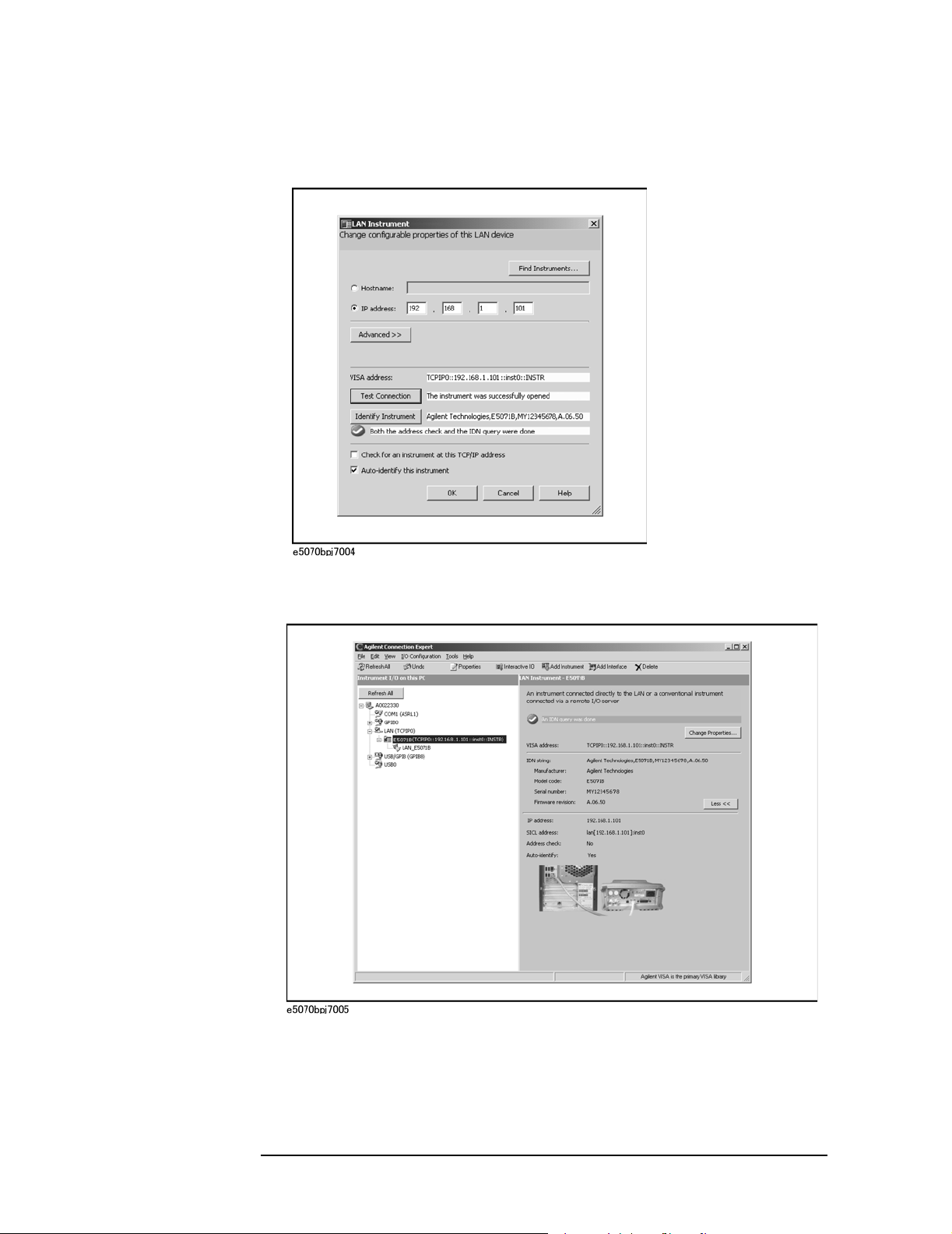
Overview of Remote Control

LAN remote control system

Step 4. In the LAN Instrument Properties screen, set up the IP address of the E5070B/E5071B and

click

OK.You can change settin gs as necessary. For details, refer to the Agilent I/O

Libraries Suite manual.

Step 5. In the Agilent Connection Expert screen, check that the E5070B/E50 71B has been added

under

LAN(TCPIP0) in the Instrument I/O on this PC frame.

36 Chapter 2

Overview of Remote Control

LAN remote control system

Control using C or Visual Basic

You can control the E5070B/E5071B by programming using SICL with the C language in the UNIX environment, or Visual C++ or Visual Basic in the Windows environment.

For more information on the control method, see a sample program using the VBA macro of Microsoft Excel described in “Control Using SICL-LAN Server” on page 265.

Control using Agilent VEE

Agilent VEE allows you to control the E5070B/E5071B via the I/O interface. The following example shows how to control the E5070B/E5071B that is set as follows: the address of the SICL-LAN server is 17 and the IP address is 192.168.0.1.

NOTE When using Agilent VEE for PC, use Agilent VEE Pro 6 for Windows or later.

2. Overview of Remote

Control

Step 1. On the Agilent EVE’s Step 2. In the Instrument Manager setting screen, click

I/O menu, click Instrument Manager....

Add....

Step 3. The Instrument Properties setting screen appear. Make the settings as follows: Name (1 in

the figure below): below):

GPIB, and Address (3 in the figure below): 917 (for the E5070B/E5071B, fixed to

9. 17 is the address of the SICL-LAN server). Then, click Gateway:

SICL_LAN (you can specify any name), Interface (2 in the figure

This host. The Select

or Enter Gateway setting screen appears. Enter the IP address or host name of the E5070B/E5071B (4 in the figure below).

Figure 2-3 shows an example of control using the I/O interface that has been set in the above procedure.

Chapter 2 37

Overview of Remote Control

LAN remote control system

Figure 2-3 Example of control using Agilent VEE

38 Chapter 2

Overview of Remote Control

LAN remote control system

Control over telnet server

In the control system over telnet server, communications are performed through connection between the sockets provided by the processes of the external controller and the E5070B/E5071B to establish a network path between them.

A socket is an endpoint for network connection; port 23 and port 5025 are provided for the sockets for the E5070B/E5071B. Port 23 is provided for conversational control using telnet (user interface program for the TELNET protocol) and port 5025 for control from a program.

Preparing the E5070B/E5071B

T o communicate with the external controller, follow these steps to turn on the telnet server of the E5070B/E5071B in advance.

[System] - Misc Setup - Network Setup - Telnet Server [ON]

2. Overview of Remote

Control

Chapter 2 39

Overview of Remote Control

LAN remote control system

Conversational control using telnet (using port 23)

You can use telnet to pe rform conversational control by sending SCPI commands to the E5070B/E5071B on a message-by-message basis. For telnet, the socket of port 23 is used for communications.

In this example, in order to show you the control procedure using telnet, you control the E5070B/E5071B (IP address: 192.168.0.1 and host name: e5070a) from the external controller in the Windows environment.

Step 1. Open the MS-DOS command prompt screen. Step 2. At the MS-DOS prompt, type telnet 192.168.0.1 or telnet e5070a and press the return key. Step 3. The telnet screen opens. Step 4. Type a command and press the return key; it is sent to the E5070B/E5071B and executed.

If you enter a command that queries some data, the query response is displayed below the line you have entered the command.

Figure 2-4 shows the screen after using the :SYST:PRES command on page 796 to reset, the :SENS{1-16}:FREQ:STAR command on page 657 and :SENS{1-16}:FREQ:STOP command on page 658 commands to set the sweep start value and stop value to 1 GHz and 2 GHz respectively, and checking the settings.

Figure 2-4 Example of control using telnet

Step 5. Select Disconnect from the Connect menu in the telnet screen (1 in Figure 2-4) to break the

connection to the E5070B/E5071B and select Exit from the Edit menu to exit the telnet. (In other environment such as the UNIX environment, press ] while holding down the control key. The telnet prompt appears. At the telnet prompt, type quit and press the return key. The connection to the E5070B/E5071B breaks and telnet finishes.)

40 Chapter 2

Overview of Remote Control

LAN remote control system

Control from a program (using port 5025)

When controlling the E5070B/E5071B from a program on the external controller, use the socket of port 5025 for connection.

NOTE Some functions such as service requests that are available in the GPIB remote control

system are not available in control over telnet server.

Control using C or Visual Basic

You can control th e E5070B/ E5 071B by socket programming using the C language in the UNIX environment, or Visual C++ or Visual Basic in the Windows environment.

For socket programming, the library for network connection on the TCP/IP protocol is required. For the UNIX environment, BSD (Berkeley Software Distribution) Sockets API is available; for the Windows environment, WinSock (WinSock1.1 and WinSock2.0) created by porting BSD Sockets to Windows and expanding it is available.

For more information on the control method, see a sample program for control using WinSock described in “Controlling Using Telnet Server” on page 273.

Agilent Control using VEE

Agilent VEE allows you to control the E5070B/E5071B through the connection to the socket of port 5025 using To/From Socket. Figure 2-5 shows an example (when the IP address of the E5070B/E5071B is 192.168.0.1). Enter 5025 in the field to specify the port for connection (1 in Figure 2-5) and enter the IP address or host name of the E5070B/E5071B in the filed to specify the host name (2 in Figure 2-5).

Figure 2-5 Example of control using Agilent VEE

2. Overview of Remote

Control

Chapter 2 41

Overview of Remote Control

USB Remote Control System

The USB (Universal Serial Bus) remote control system provides device control via USB that is equivalent to control via GRIP. Connection is made through an interface in compliance with USBTMC-USB488 and USB 2.0.

System configuration

The USB remote control system controls instruments that use the name “alias.” There is no such address for GPIB connections.

Use a LAN cable to connect the E5070B/E5071B to an external controller (personal computer). Figure 2-6 shows an overview of the system configuration for the USB remote control system.

Figure 2-6 USB Remote Control System Configuration

Required Equipment

1. E5070B/E5071B (models with USB (USBTMC) interface port (type B)).

2. External controller (personal computer with installed Agilent I/O Li braries and USB host port (type A)).

3. Other USB compatible devices (instruments and/or peripherals for specific purposes).

4. USB cable connecting E5070B/E5071B and external controller (with type A/4-prong male or type B/4-prong male connectors depending on device used).

USB Port Types

There are two standard types of USB ports. The external controller (PC) must be connected

42 Chapter 2

Overview of Remote Control

USB Remote Control System

via the USB host port (type A), while the E5070B/E5071B and other USB compatible devices must be connected via the USB interface port (type B).

Type A: USB host port

Type B: USB (USBTMC) interface port

Preparing E5070B/E5071B

You do no t have to configu re any softkey or co mm and of the E5070B/E5071B in order to control the E5070B/E5071B from an external controller. Simply connect a USB cable to the USB interface port.

Preparing External Controller

In order to establish communication with the E5070B/E5071B via USB, you must set up the I/O interface of the external controller in advance. The USB can identify devices automatically, so once you connect a USB cable to a tar get device, a dialog box will appear for USB device registration.

2. Overview of Remote

Control

NOTE The E5070B/E5071B will be identified as new device if its serial number has been

changed.

NOTE You must install the Agilent I/O Libraries in advance. Use Agilent I/O Libraries M.01.01

or Agilent I/O Libraries Suite 14 or later. For further information on the I/O Libraries, see the Agilent I/O Libraries Manual. The Agilent I/O Libraries may not be available for certain external controllers or OS

versions. For further details, refer to the Help guidance for the Agilent I/O Libraries.

Chapter 2 43

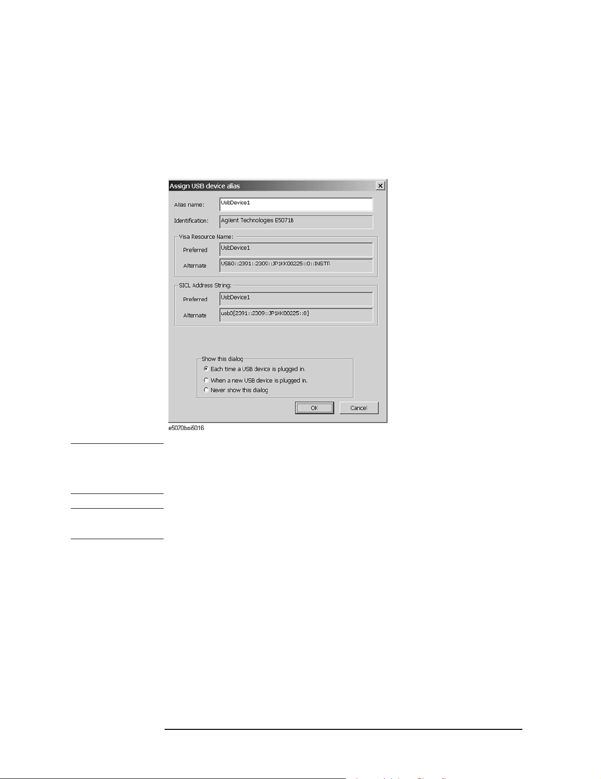
Overview of Remote Control

USB Remote Control System

1. Registering Alias When USB Cable Is Connected

When new device is connected via USB cable, the following dialog box will appear automatically.Follow the steps below to register alias, when you use the Agilent I/O Libraries Suite 14.

Step 1. In the Assign USB device alias dialog box, enter an alias and the click the

Figure 2-7 Registering Alias

OK button.

NOTE For alias, use the ASCII format less than 127 digits.Alias is upper/lower case insensitive.

If "Never show this dialog" is selected in the "Show this dialog" frame, the dialog box does not appear even if a new device is connected.

NOTE Once new device is identified, the "New Hardware Search Wizard" will start.Follow the

instruction to implement the processing.

2. Changing Alias on Setting Screen

The following are steps using the Agilent I/O Libraries Suite 14.

Step 1. Step 1: From the Start menu of your PC, click Program - Agilent IO Libraries Suite

-Agilent Connection Expert to open the Config setting screen.

Step 2. In the Config setting screen, select the alias names from

I/O on this PC

frame, and then use the Change Properties from I/O Configuration on the

USB0 onward in the Instrument

menu bar.

44 Chapter 2

Figure 2-8 Changing Alias

Overview of Remote Control

USB Remote Control System

2. Overview of Remote

Control

Control using C or Visual Basic

You can control the E5070B/E5071B by programming using Visual C++ or Visual Basic in the Windows environment as well as SICL/VISA.For further information on controlling the E5070B/E5071B, see the manual of SICL or VISA.For Agilent I/O Libraries, use Agilent I/O Libraries M.01.01 or Agilent I/O Libraries Suite 14.

You may use alias in the prog ramming using SICL/VISA. The following example shows an OPEN command to control the E5070B/E5071B to

which alias is given as ENA_USBIF.

SICL id = iopen("ENA_USBIF") VISA viOpen(...,"ENA_USBIF",...)

NOTE For further details of the programming using SICL/VISA, see the SICL Users Guide or the

VISA Users Guide.

Chapter 2 45

Overview of Remote Control

USB Remote Control System

Control using Agilent VEE

Agilent VEE allows you to control the E5070B/E5071B via the direct I/O interface.The following example shows how to control the E5070B/E5071B to which alias is given as ENA_USBIF.

NOTE When using Agilent VEE for PC, use Agilent VEE Pro 7 for Windows or later version.

Step 1. On the Agilent VEE's Step 2. In the Instrument Manager setting screen, click

I/O menu, click Instrument Manager....

Add....

Step 3. The Instrument Properties dialog box appears.Specify Name:

any other name acceptable), Interface: below, USB port number), and Alias: the IO Config setting screen), then click

USB(2 shown below), Board Number :0(3 shown

ENA_USBIF(4 shown below which is registered in

OK.

ENA_USBIF(1 shown below,

Figure 2-9shows an example of control using the direct I/O interface that has been set in the above procedures.

46 Chapter 2

Figure 2-9 Sample Control Using Agilent VEE (USB)

Overview of Remote Control

USB Remote Control System

2. Overview of Remote

Control

Chapter 2 47

Overview of Remote Control

Sending SCPI command messages

Types and structure of commands

The SCPI commands available for the E5070B/E5071B are classified into 2 groups as follows.

E5070B/E5071B commands

Commands specific to the E5070B/E5071B. They cover all measurement functions that the E5070B/E5071B has and some general-purpose functions. The commands in this group are arranged in a hierarchical structure called the command tree (see “Command tree” on page 828). Each command consists of character strings (mnemonics) indicating each hierarchical level and colon (:) separators between hierarchical levels.

IEEE common commands

Commands to cover general-purpose functions defined in IEEE488.2 that are available commonly to instruments that support this standard. The commands in this group have an asterisk (*) at the beginning. For the commands in this group, there is no hierarchical structure.

Concepts of the command tree

The commands at the top of the command tree are called “root command” or simply “root.” To access lower level commands in the tree, you need to specify a specific path like a directory path in the DOS file system. After po wer-on or reset, the current path is set to the root. Special characters in messages change the path setting as described below.

Message terminator A message terminator such as the

<new line> character sets the current path to the root.

Colon (:) A colon between 2 command mnemonics lowers the level of the

current path in the command tree. A colon used as the first character of a command specifies the command mnemonic that follows as the root-level command.

Semicolon (;) A semicolon does not change the current path and separates 2

commands in the same message.

Figure 2-10 shows an example of how to use colons and semicolons to efficiently access commands in the command tree.

48 Chapter 2

Figure 2-10 Using colons and semicolons

Overview of Remote Control

Sending SCPI command messages

2. Overview of Remote

Control

Grammar of messages

This section describes the grammar to send program messages via GPIB. Program messages are messages that the user sends to the instrument from the external controller to control the instrument. A program message consists of 1 or more commands and their necessary parameters.

Upper/lower case sensitivity

Upper/lower case insensitive.

Program message terminator

A program message must be terminated with one of the 3 program message terminators: <new line>, <^END>, or <new line><^END>. <^END> indicates that EOI on the GPIB interface becomes active at the instant when the immediately previous data byte is sent. For example, the OUTPUT command of HTBasic automatically sends the message terminator after the last data byte.

Parameters

A space (ASCII code: 32) is required between a command and its first parameter. When sending several parameters in a single command, separate each parameter with a comma (,).

Message including several commands

When sending 2 or more commands in a single message, separate each command with a semicolon (;). The following example shows how to send the *CLS command and the :STAT:PRES command in a single message using HTBasic.

OUTPUT 717;"*CLS;:STAT:PRES"

Chapter 2 49

Overview of Remote Control

Sending SCPI command messages

Remote mode

The E5070B/E5071B does not provide remote mode. Therefore, even if you send a GPIB command, it never enters into remote mode automatically. There is no local key to release remote mode.

If you need to prevent misoperation during remote control due to entry from the front panel or mouse, lock the input devices using the following commands.

• :SYST:KLOC:KBD command on page 794

• :SYST:KLOC:MOU S command on page 795

50 Chapter 2

3 Setting Up the Analyzer

3. Setting Up the Analyzer

This chapter describes how to configure measurement conditions and how to configure the way the instrument displays measurement results on the LCD.

Setting Up the Analyzer

Selecting the Active Channel/Trace

You can configure the E5070 B/E507 1B by using various commands. Some commands require you to specify and work with a particular channel or trace, while other commands do not have this restriction.

Those commands that do not require you to specify a particular channel or trace apply to the currently active channels and traces. Before issuing such a command, therefore, you must make the appropriate channels and traces active.

To make a channel active, use the following command:

• :DISP:WIND{1-16}:ACT on page 470

NOTE Only the currently displayed channels can be active channels. Therefore, you must display

the desired channels by using the :DISP:SPL command on page 466 before making them active.

To make a trace active, use the following command:

• :CALC{1-16}:PAR{1-16}:SEL on page 424

NOTE Only the currently displayed traces can be active traces. Therefore, you must display the

desired traces by using the :CALC{1-16}:PAR:COUN command on page 421 before making them active.

52 Chapter 3

Setting Up the Analyzer

Configuring Measurement Conditions

Setting the number of traces

When you set the number of traces, that setting determines the upper limit trace number; for example, if the setting is 3, traces 1 through 3 will be displayed. To set the number of traces, use the following command:

• :CALC{1-16}:PAR:COUN on page 421

NOTE Only the currently displayed traces can be active traces. Therefore, you must set the

number of traces appropriately before making them active.

Selecting measurement parameters

To select the measurement parameter (S parameter) for each trace, use the following command:

• :CALC{1-16}:PAR{1-16}:DEF on page 422 When you use the Balance-Unbalance Conversion feature, you can select the mixed mode

S parameter as well. For more information, refer to “Analysis Using the Fixture Simulator” on page 150.

Setting the sweep condition (Stimulus)

How you can set the sweep condition depends on the sweep type. You can choose between the following four sweep types:

• Linear sweep

• Log sweep

• Segment sweep

• Power sweep To select one of the above sweep types, use the following command:

• :SENS{1-16}:SWE:TYPE on page 696 To select the sweep mode (stepped/fast stepped/swept/fast swept), use the following

command:

• :SENS{1-16}:SWE:GEN on page 692

3. Setting Up the Analyzer

Turning On/Off stimulus signal output

T o turn on/off the stimulus signal output, use the following commands. For example, if the power output is automatically turned off due to the power trip feature, remove the cause of the over-input and turn on the stimulus signal output by executing the following command. You canno t pe rform measurement until you turn on the stimulus signal output.

• :OUTP on page 527

Chapter 3 53

Setting Up the Analyzer

Configuring Measurement Conditions

Configuring linear sweep settings

To set the sweep range, use the following commands:

Start value :SENS{1-16}:FREQ:STAR on page 657 Stop value :SENS{1-16}:FREQ:STOP on page 658 Center value :SENS{1-16}:FREQ:CENT on page 654 Span value :SENS{1-16}:FREQ:SPAN on page 656

To set the number of measurement points, use the following command:

• :SENS{1-16}:SWE:POIN on page 693

To set the measurement time, use the following commands:

Measurement time :SENS{1-16}:SWE:TIME on page 694 Turning on/off auto setting :SENS{1-16}:SWE:TIME:AUTO on page 695

To set the sweep delay time, use the following command:

• :SENS{1-16}:SWE:DEL on page 691

To set the IF bandwidth, use the one of the following commands (both provide the same function):

• :SENS{1-16}:BAND on page 545

• :SENS{1-16}:BWID on page 546

Setting power level

When the instrument is equipped with the power range expansion function (Option 214, 314, or 414), you can select the power range by using the following command:

• :SOUR{1-16}:POW:ATT on page 705

To set the power level, use the following command:

• :SOUR{1-16}:POW on page 704

To select whether to output the same power level (the set value for port 1) or a different power level for each port, use the following command:

• :SOUR{1-16}:POW:PORT:COUP on page 709

• :SOUR{1-16}:POW:PORT{1-4} on page 710

To set the correction of power-level attenuation so that it’s proportional to the frequency (power slope feature), use the following command:

• :SOUR{1-16}:POW:SLOP:STAT on page 718

• :SOUR{1-16}:POW:SLOP on page 71 7

NOTE If you turn on the power slope feature, the sweep mode is changed to the step mode.

54 Chapter 3

Setting Up the Analyzer

Configuring Measurement Conditions

Configuring segment sweep settings

When you opt to use segment sweep, you can set all items (in the segment sweep table) by using a single command:

• :SENS{1-16}:SEGM:DATA on page 688 Alternatively, you can configure the segment sweep settings based on the data contained in

a CSV file by issuing the following command:

• :MMEM:LOAD:SEGM on page 504 Also, you can save the contents of the current segment sweep table to a file by issuing the

following command:

• :MMEM:STOR:SEGM on page 518 For more information on how to save and load the segment sweep table, refer to “Saving

and recalling the segment sweep table.”

Configuring power sweep settings

To set the sweep range, use the following commands:

Start value :SOUR{1-16}:POW:STAR on page 720 Stop value :SOUR{1-16}:POW:STOP on page 721 Center value :SOUR{1-16}:POW:CENT on page 708 Span value :SOUR{1-16}:POW:SPAN on page 719

To set the fixed frequency (CW frequency), use the following command:

• :SENS{1-16}:FREQ on page 653 To set the number of points, the sweep time, the sweep delay time, and the IF bandwidth,

use the same commands as for the linear/log sweep.

Configuring Averaging Settings

To configure the smoothing settings, use the following commands:

On/off :SENS{1-16}:AVER on page 543 Averaging factor :SENS{1-16}:AVER:COUN on page 544 Clear (Restart) :SENS{1-16}:AVER:CLE on page 543

For averaging, normally, the instrument must be triggered according to the number of averaging; however, when the averaging trigger is turned on, sweeps for the number of averaging can be executed by a single trigger. For details on the averaging trigger, refer to “Averaging Trigger Function” on page 138 of Chapter 5, “Making a Measurement,”

3. Setting Up the Analyzer

Chapter 3 55

Setting Up the Analyzer

Configuring Measurement Conditions

Setting the System Z0

NOTE This function is available with the firmware version 3.01 or greater.

To set the system characteristic impedance (Z0), use the following command:

• :SENS:CORR:IMP on page 537

56 Chapter 3

Setting Up the Analyzer

Configuring Display Settings

Setting the layout of windows and graphs

You can sp lit the E5070B/E5071B’s LCD screen into multiple windows that display channel-specific result information, and the window layout can be selected from a number of variations. In addition, you can place on screen a segment sweep table or echo window, which you can use to display messages from your custom program.

Selecting the window layout (Channel Display Mode)

One window displays the results for a single channel. You cannot have a single window display the results from more than one channel. This means that setting the window layout determines the number of channels displayed on screen.

To select one of the 19 different window layouts shown in Figure 3-1, use the following command:

• :DISP:SPL on page 466

Selecting the graph layout (Trace Display Mode)

3. Setting Up the Analyzer

You can place a number of trace graphs in each window by selecting one of the pre-defined graph layouts. The number of graphs differs depending on your selected graph layout. If the number of graphs is equal to or larger than the number of traces (set by the :CALC{1-16}:PAR:COUN command on page 421), each graph always displays one trace. On the other hand, if the number of graphs is smaller than the number of traces, some of the graphs display two or more traces. Graph 1 is populated with trace 1, graph 2 with trace 2, and so on. Traces whose numbers exceed the last graph's number will populate graph 1, graph 2, and so on.

To select one of the 19 different graph layouts shown in Figure 3-1, use the following command:

• :DISP:WIND{1-16}:SPL on page 475

Maximizing a window or a trace graph

When you have multiple windows displayed, you can maximize the active channel window so that it covers the entire screen area. To maximize a window, use the following command:

• :DISP:MAX on page 465 Similarly, when you have multiple traces displayed, you can maximize the active trace so

that it extends throughout the entire window. To maximize a trace, use the following command:

• :DISP:WIND{1-16}:MAX on page 474

Chapter 3 57

Setting Up the Analyzer

Configuring Display Settings

Figure 3-1 Window/graph layouts and command parameters

58 Chapter 3

Setting Up the Analyzer

Configuring Display Settings

Showing/hiding a table or echo window

You can displ ay the fol lowing items at the bottom of the LCD screen:

• Segment sweep table

• Limit table

• Marker list table

• Echo window (a window that displays messages from a custom program)

• Loss compensation table

• Power sensor’s calibration factor table To show or hide each of the above items, use the following command:

• :DISP:TABL on page 468 You can have two or more of the above items displayed at a time. The screen displays only

the selected item by using the following command:

• :DISP:TABL:TYPE on page 469

Showing/hiding softkey labels

You can show or hide the softkey labels placed alongside the right-hand edge of the LCD screen. To show or hide the softkey labels, use the following command:

• :DISP:SKEY on page 465

3. Setting Up the Analyzer

Chapter 3 59

Setting Up the Analyzer

Configuring Display Settings

Configuring trace display settings

Selecting which traces to display

Each trace has two different representations: data and memory traces. You can show or hide the data and memory traces independently of each other. To show or hide the data or memory traces, use the following commands:

Data trace :DISP:WIND{1-16}:TRAC{1-16}:STAT on page 481 Memory trace :DISP:WIND{1-16}:TRAC{1-16}:ANN:MARK:POS:X on

page 478

To copy the data trace to the memory trace, use the following command:

• :CALC{1-16}:MATH:MEM on page 416

Configuring cross-trace math operations

You can perform math operations between the data and memory traces and have the results displayed as the data trace. To perform cross-trace math operations, use the following command:

• :CALC{1-16}:MATH:FUNC on page 415

Configuring smoothing settings

To turn on/off smoothing, use the following command:

• :CALC{1-16}:SMO on page 433

The smoothing aperture is expressed as a percentage with respect to the sweep range. To set the smoothing aperture, use the following command:

• :CALC{1-16}:SMO:APER on page 434

Selecting the data format

You can select the following data formats: R Rectangular display formats

• Log magnitude format

•Phase format

• Group delay format

• Linear magnitude format

• SWR format

• Real format

• Imaginary format

• Expanded phase format

• Positive phase format

R Imaginary format R Expanded phase format

To select the measurement parameter data format, use the following command:

60 Chapter 3

• :CALC{1-16}:FORM on page 321

Setting Up the Analyzer

Configuring Display Settings

3. Setting Up the Analyzer

Chapter 3 61

Setting Up the Analyzer

Configuring Display Settings

Configuring the display scale

Depending on the measurement parameter data format, you can configure the display scale in one of the following two ways:

Rectangular display formats:

When you use one of rectangular display formats (Logarithmic magnitude/Phase/ Group delay/Linear magnitude/SWR/Real/Imaginary/Expanded phase/Positive phase), you can configure the display scale by setting the following four items:

Number of divisions :DISP:WIND{1-16}:Y:DIV on page 486 Scale per division :DISP:WIND{1-16}:TRAC{1-16}:Y:PDIV on page 482 Reference graticule line :DISP:WIND{1-16}:TRAC{1-16}:Y:RPOS on page484 Reference graticule line value :DISP:WIND{1-16}:TRAC{1-16}:Y:RLEV on page 483

NOTE The number of divisions is a channel-wide setting (shared among all traces), while the

remaining three settings are trace-specific.

You can sh ow or hide graticule label (the label on the left-hand side of the graticule lines) by issuing the following command:

• :DISP:WIND{1-16}:LAB on page 473

Smith chart/Polar formats:

When you are using one of Smith chart/Polar formats, you can only set the full scale value (the outermost circle’s value) using the following command:

• :DISP:WIND{1-16}:TRAC{1-16}:Y:PDIV on page 482

Auto Scale

You can use Auto Scale to automatically set the display scale. This feature works by automatically adjusting the reference division line value and the scale value per division when you are using one of the rectangular display formats or the full scale value when you are using one of Smith chart/Polar formats.

To perform Auto Scale, use the following command:

• :DISP:WIND{1-16}:TRAC{1-16}:Y:AUTO on page 481

62 Chapter 3

Setting Up the Analyzer

Configuring Display Settings

Printing a message in the echo window

You can pri nt a message in the echo wi ndow by issuing the following command:

• :DISP:ECHO on page 461 You can clear any m essage displayed in the echo window by issuing the following

command:

• :DISP:ECHO:CLE on page 461

Turning On/Off display update

To turn on/off the update of the LCD screen, use the following command:

• :DISP:ENAB on page 462

Showing/hiding frequencies

To show or hide frequencies on the LCD screen, use the following command:

• :DISP:ANN:FREQ on page 454

Showing or hiding the title

3. Setting Up the Analyzer

To show or hide the title, use the following command:

• :DISP:WIND{1-16}:TITL on page 476 To define the title string that appears in the title display area, use the following command:

• :DISP:WIND{1-16}:TITL:DATA on page 477

Configuring date/time display

T o show or hide the current date and time on the left-hand side of the instrument status bar, use the following command:

• :DISP:CLOC on page 455 To set the date and time, use the following command:

• :SYST:DATE on page 790

• :SYST:UPR on page 801

Turning On/Off the LCD backlight

To turn on/off the LCD backlight, use the following command (note that turning off the backlight makes the screen unreadable):

• :SYST:BACK on page 779

Chapter 3 63

Setting Up the Analyzer

Configuring Display Settings

Setting display colors

Selecting display mode

You can sel ect the one of two LCD displ a y modes: normal display (black background) or inverted display (white background).

To select the display mode, use the following command:

• :DISP:IMAG on page 464

Setting display color for each item

To set the display colors, use the following commands:

Data trace :DISP:COL{1-2}:TRAC{1-16}:DATA on page 459 Memory trace :DISP:COL{1-2}:TRAC{1-16}:MEM on page 460 Graph :DISP:COL{1-2}:GRAT{1-2} on page 457 Limit test :DISP:COL{1-2}:LIM{1-2} on page458 Background :DISP:COL{1-2}:BACK on page 456

Resetting display colors to factory state

You can reset the display colors in normal display and inverted display to the preset factory state.

To reset the display colors, use the following command:

• :DISP:COL{1-2}:RES on page 458

64 Chapter 3

Setting Up the Analyzer

Saving and Loading the Settings

You can save the settings for measurement conditions and screen disp lay to a file along with other instrument settings, and these settings can later be loaded from the file.

Once you have saved the measurement condition and screen display settings to a file, you can later load them whenever necessary; therefore, you can quickly modify the settings loaded from a file to create new settings without having to issue many commands.

To save the current settings to a file, use the following command:

• :MMEM:STOR on page 506 To load the settings from a file, use the following command:

• :MMEM:LOAD on page 495 For more information on how to save and load the settings, refer to “Saving and recalling

instrument status.”

3. Setting Up the Analyzer

Chapter 3 65

Setting Up the Analyzer

Sample Program

Example 3-1 is a sample program that demonstrates how to configure measurement conditions. You can find the source file of this program, named setup.htb, on the sample program disk.

The sample program puts the instrument into the preset state, configures it as shown in Table 3-1, and saves the settings to a file named “Ex_3_1.sta”.

Table 3-1 Target settings in Example 3-1

Item Setting

Window Layout Channel 1 in the upper

Channel 1 Sweep type Segment

Sweep range See Table 3-2. Number of measurement points IF bandwidth Power Number of traces 4 Graph Layout Four graphs at upper left,

Trace 1 Measurement parameter S11

Trace 2 Measurement parameter S21

Trace 3 Measurement parameter S12

Trace 4 Measurement parameter S22

window (2/3 of the screen height) and channel 2 in the lower window (1/3 of the screen height)

upper right, lower left, and lower right.

Data format Smith chart (Lin) Full-scale value 2

Data format Log magnitude Reference division line

number Reference division line

value Scale per division 10 dBm

Data format Log magnitude Reference division line

number Reference division line

value Scale per division 10 dBm

Data format Smith chart (Lin) Full-scale value 2

66 Chapter 3

Table 3-1 Target settings in Example 3-1

Item Setting

Channel 2 Sweep type Linear

Sweep range Center value 1.9 GHz

Number of measurement points 101 IF bandwidth 70 kHz Power 0 dBm Number of traces 4 Graph Layout Two graphs at left and right Trace 1 Measurement parameter S21

Trace 2 Measurement parameter S22

Setting Up the Analyzer

Sample Program

Span value 500 MHz

Data format Log magnitude Reference division line

number Reference division line

value Scale per division 10 dBm

Data format Smith chart (Lin) Full-scale value 2

3. Setting Up the Analyzer

Table 3-2 Segment table for channel 1

Segment Number

1 1.7 GHz 1.9 GHz 21 50 kHz 0 dBm 2 1.9 GHz 2 GHz 101 10 kHz -10 dBm 3 2 GHz 2.2 GHz 21 50 kHz 0 dBm

Start value Stop value

Number of

measurement

points

IF bandwidth Power

Chapter 3 67

Setting Up the Analyzer

Sample Program

The program is described in detail below: Line 70 Assigns a GPIB address to the I/O pass. Line 90 Stores the number of channel 1’s sweep segments into the Segm

variable.

Lines 100 to 150 These lines store the start and stop values for channel 1’s segments 1

through 3 into the Star1(*) and Stop1(*) variables, respectively.

Lines 160 to 170 These lines store channel 2’s center and span values into the Star2 and

Stop2 variables, respectively.

Lines 180 to 210 These lines store the number of points for channel 1’s segments 1

through 3 into the Nop1(*) variable and the number of measurement points for channel 2 into the Nop2 variable.

Lines 220 to 250 These lines store the IF bandwidth for channel 1’s segments 1 through

3 into the If_bw1(*) variable and the IF bandwidth for channel 2 into the If_bw2 variable.

Lines 260 to 290 These lines store the power for channel 1’s segments 1 through 3 into

the Pow1(*) variable and the power for channel 2 into the Pow2 variable.

Lines 300 to 310 These lines store the number of channel 1’s traces into the Num_of_tr1

variable and the number of channel 2’s traces into the Num_of_tr2 variable.

Lines 320 to 330 These lines store channel 1’s graph layout into the Allocate1$ variable

and channel 2’s graph layout into the Allocate2$ variable.

Lines 340 to 390 These lines store the measurement parameters for channel 1’s traces 1

through 4 into the Para1$(*) variable and the measurement parameters for channel 2’s traces 1 through 2 into the Para2$(*) variable.

Lines 400 to 450 These lines store the data formats for chann e l 1’s traces 1 through 4

into the Fmt1$(*) variable and the data formats for channel 2’s traces 1 through 2 into the Fmt2$(*) variable.

Lines 460 to 480 These lines store the reference division line numbers for channel 1’s

traces 2 through 3 into the Ref_pos1(*) variable and the reference division line numbers for channel 2's trace 1 into the Ref_pos2(*) variable.

Lines 490 to 510 These lines store the reference division line values for channel 1’s

traces 2 through 3 into the Ref_lev1(*) variable and the reference division line values for channel 2’s trace 1 into the Ref_lev2(*) variable.

Lines 520 to 570 These lines store the data formats for chann e l 1’s traces 1 through 4

into the Fmt1$(*) variable and the data formats for channel 2’s traces 1

through 2 into the Fmt2$(*) variable. Line 580 Stores the name of the file into the File$ variable. Line 600 Puts the instrument into preset state. Line 620 Places the window for channel 1 in the upper part of the LCD screen

and the window for channel 2 in the lower part. Lines 630 to 640 These lines turn on Continuous Acti vation mode for channels 1 and 2.

68 Chapter 3

Setting Up the Analyzer

Sample Program

Line 680 Sets channel 1’s sweep type to “segment”. Lines 690 to 730 These lines set up the segment table for channel 1.

Line 600: Sends the command that sets up the segment table along with the parameter header (“5,0,1,1,0,0” causes the IF bandwidth and power to be set on a segment-by-segment basis; Segm represents the number of segments).

Lines 700 to 730: Send the data for the start and stop values, number of points, IF bandwidth, and power (Star1, Stop1, Nop1, If_bw1, Pow1) on a segment-by-segment basis.

Lines 750 to 760 For channel 1, these lines set the number of traces to Num_of_tr1 and

the graph layout to Allocate1$.

Lines 770 to 890 For channel 1, the program iterates the following loop while

incrementing i from 1 to Num_of_tr1 for each trace.

Line 780: Sets the measurement parameter to Para1$(i). Line 790: Makes trace(i) active. Line 800: Sets the data format to Fmt1$(i). Line 830: If the data format is Smith chart or polar, this line sets

the full-scale value to Scale1(i).

3. Setting Up the Analyzer

Lines 850 to 870: If the data format is neither Smith chart nor polar, these lines set the reference division line number to Ref_pos1(i), the reference division line value to Ref_lev1(i), and

the scale per division to Scale1(i). Line 930 Sets channel 2’s sweep type to “linear”. Lines 940 to 980 For channel 2, these lines set the center value to Cent2, the span value

to Span2, the number of measurement points to Nop2, the IF bandwidth to If_bw2, and the power to Pow2.

Lines 1000 to 1010 For channel 2, these lines set the number of traces to Num_of_tr2 and

the graph layout to Allocate2$.

Lines 1020 to 1140 For channel 2, the program iterates the following loop while

incrementing i from 1 to Num_of_tr2 for each trace.

Line 1030: Sets the measurement parameter to Para2$(i).

Line 1040: Makes trace(i) active.

Line 1050: Sets the data format to Fmt2$(i).

Line 1080: If the data format is Smith chart or polar, this line sets

the full-scale value to Scale2(i).

Lines 1100 to 1120: If the data format is neither Smith chart nor

polar, these lines set the reference division line number to

Ref_pos2(i), the reference division line value to Ref_lev2(i), and

the scale per division to Scale2(i). Line 1160 Saves the settings of the E5070B/E5071B under the file name File$.

Chapter 3 69

Setting Up the Analyzer

Sample Program

Example 3-1 Configuring measurement conditions (setup.htb)

10 DIM Allocate1$[9],Allocate2$[9],File$[20] 20 DIM Para1$(1:4)[9],Para2$(1:2)[9],Fmt1$(1:4)[9],Fmt2$(1:2)[9] 30 REAL Star1(1:3),Stop1(1:3),Pow1(1:3),Cent2,Span2,Pow2 40 REAL Ref_rev1(1:4),Ref_rev2(1:2),Scale1(1:4),Scale2(1:2) 50 INTEGER Segm,Nop1(1:3),Nop2,Num_of_tr1,Num_of_tr2 60 INTEGER Ref_pos1(1:4),Ref_pos2(1:2),I 70 ASSIGN @Agte507x TO 717 80 ! 90 Segm=3 ! Number of Segment Ch.1 : 3 100 Star1(1)=1.7E+9 ! Start Frequency Ch.1 Segm.1: 1.7 GHz 110 Star1(2)=1.9E+9 ! Segm.2: 1.9 GHz 120 Star1(3)=2.E+9 ! Segm.3: 2 GHz 130 Stop1(1)=1.9E+9 ! Stop Frequency Ch.1 Segm.1: 1.9 GHz 140 Stop1(2)=2.E+9 ! Segm.2: 2 GHz 150 Stop1(3)=2.2E+9 ! Segm.3: 2.2 GHz 160 Cent2=1.9E+9 ! Center Frequency Ch.2 : 1.9 GHz 170 Span2=5.00E+8 ! Span Ch.2 : 500 MHz 180 Nop1(1)=21 ! Number Ch.1 Segm.1: 21 190 Nop1(2)=101 ! of Points Segm.2: 101 200 Nop1(3)=21 ! Segm.3: 21 210 Nop2=101 ! Ch.2 : 101 220 If_bw1(1)=5.0E+4 ! IF Bandwidth Ch.1 Segm.1: 50 kHz 230 If_bw1(2)=1.0E+4 ! Segm.2: 10 kHz 240 If_bw1(3)=5.0E+4 ! Segm.3: 50 kHz 250 If_bw2=7.0E+4 ! Ch.2 : 70 kHz 260 Pow1(1)=0 ! Power Ch.1 Segm.1: 0 dBm 270 Pow1(2)=-10 ! Segm.2: -10 dBm 280 Pow1(3)=0 ! Segm.3: 0 dBm 290 Pow2=0 ! Ch.2 : 0 dBm 300 Num_of_tr1=4 ! Number Ch.1 : 4 310 Num_of_tr2=2 ! of Traces Ch.2 : 2 320 Allocate1$="D12_34" ! Allocate Traces Ch.1 : D12_34 330 Allocate2$="D12" ! Ch.2 : D12 340 Para1$(1)="S11" ! Measurement Ch.1 Trace1: S11 350 Para1$(2)="S21" ! Parameter Trace2: S21 360 Para1$(3)="S12" ! Trace3: S12 370 Para1$(4)="S22" ! Trace4: S22 380 Para2$(1)="S31" ! Ch.2 Trace1: S31 390 Para2$(2)="S33" ! Trace2: S33 400 Fmt1$(1)="SLIN" ! Data Format Ch.1 Trace1: Smith 410 Fmt1$(2)="MLOG" ! Trace2: Log Mag 420 Fmt1$(3)="MLOG" ! Trace3: Log Mag 430 Fmt1$(4)="SLIN" ! Trace4: Smith 440 Fmt2$(1)="MLOG" ! Ch.2 Trace1: Log Mag 450 Fmt2$(2)="SLIN" ! Trace2: Smith 460 Ref_pos1(2)=9 ! Reference Ch.1 Trace2: 9 470 Ref_pos1(3)=9 ! Position Trace3: 9 480 Ref_pos2(1)=9 ! Ch.2 Trace1: 9 490 Ref_lev1(2)=0 ! Reference Level Ch.1 Trace2: 0 dBm 500 Ref_lev1(3)=0 ! Trace3: 0 dBm 510 Ref_lev2(1)=0 ! Ch.2 Trace1: 0 dBm 520 Scale1(1)=2 ! Scale Ch.1 Trace1: 2 530 Scale1(2)=10 ! Trace2: 10 dBm 540 Scale1(3)=10 ! Trace3: 10 dBm 550 Scale1(4)=2 ! Trace4: 2 560 Scale2(1)=10 ! Ch.2 Trace1: 10 dBm 570 Scale2(2)=2 ! Trace2: 2 580 File$="Ex_3_1.sta" ! Save File Name : Ex_3_1.sta 590 ! 600 OUTPUT @Agte507x;":SYST:PRES" 610 ! 620 OUTPUT @Agte507x;":DISP:SPL D1_1_2" 630 OUTPUT @Agte507x;":INIT1:CONT ON" 640 OUTPUT @Agte507x;":INIT2:CONT ON"

(Lin/Phase)

70 Chapter 3

Setting Up the Analyzer

Sample Program

650 ! 660 ! Channel 1 670 ! 680 OUTPUT @Agte507x;":SENS1:SWE:TYPE SEGM" 690 OUTPUT @Agte507x;":SENS1:SEGM:DATA 5,0,1,1,0,0,";Segm;","; 700 FOR I=1 TO Segm-1 710 OUTPUT @Agte507x;Star1(I);",";Stop1(I);",";Nop1(I);",";If_bw1 (I);",";Pow1(I);","; 720 NEXT I 730 OUTPUT @Agte507x;Star1(Segm);",";Stop1(Segm);",";Nop1(Segm);"," ;If_bw1(Segm);",";Pow(Segm) 740 ! 750 OUTPUT @Agte507x;":CALC1:PAR:COUN ";Num_of_tr1 760 OUTPUT @Agte507x;":DISP:WIND1:SPL "&Allocate1$ 770 FOR I=1 TO Num_of_tr1 780 OUTPUT @Agte507x;":CALC1:PAR"&VAL$(I)&":DEF "&Para1$(I) 790 OUTPUT @Agte507x;":CALC1:PAR"&VAL$(I)&":SEL" 800 OUTPUT @Agte507x;":CALC1:FORM "&Fmt1$(I) 810 SELECT Fmt1$(I) 820 CASE "SLIN","SLOG","SCOM","SMIT","SADM","PLIN","PLOG","POL" 830 OUTPUT @Agte507x;":DISP:WIND1:TRAC"&VAL$(I)&":Y:PDIV "; Scale1(I) 840 CASE ELSE 850 OUTPUT @Agte507x;":DISP:WIND1:TRAC"&VAL$(I)&":Y:RPOS "; Ref_pos1(I) 860 OUTPUT @Agte507x;":DISP:WIND1:TRAC"&VAL$(I)&":Y:RLEV "; Ref_rev1(I) 870 OUTPUT @Agte507x;":DISP:WIND1:TRAC"&VAL$(I)&":Y:PDIV "; Scale1(I) 880 END SELECT 890 NEXT I 900 ! 910 ! Channel 2 920 ! 930 OUTPUT @Agte507x;":SENS2:SWE:TYPE LIN" 940 OUTPUT @Agte507x;":SENS2:FREQ:CENT ";Cent2 950 OUTPUT @Agte507x;":SENS2:FREQ:SPAN ";Span2 960 OUTPUT @Agte507x;":SENS2:SWE:POIN ";Nop2 970 OUTPUT @Agte507x;":SENS2:BAND ";If_bw2 980 OUTPUT @Agte507x;":SOUR2:POW ";Pow2 990 ! 1000 OUTPUT @Agte507x;":CALC2:PAR:COUN ";Num_of_tr2 1010 OUTPUT @Agte507x;":DISP:WIND2:SPL "&Allocate2$ 1020 FOR I=1 TO Num_of_tr2 1030 OUTPUT @Agte507x;":CALC2:PAR"&VAL$(I)&":DEF "&Para2$(I) 1040 OUTPUT @Agte507x;":CALC2:PAR"&VAL$(I)&":SEL" 1050 OUTPUT @Agte507x;":CALC2:FORM "&Fmt2$(I) 1060 SELECT Fmt2$(I) 1070 CASE "SLIN","SLOG","SCOM","SMIT","SADM","PLIN","PLOG","POL" 1080 OUTPUT @Agte507x;":DISP:WIND2:TRAC"&VAL$(I)&":Y:PDIV "; Scale2(I) 1090 CASE ELSE 1100 OUTPUT @Agte507x;":DISP:WIND2:TRAC"&VAL$(I)&":Y:RPOS "; Ref_pos2(I) 1110 OUTPUT @Agte507x;":DISP:WIND2:TRAC"&VAL$(I)&":Y:RLEV "; Ref_rev2(I) 1120 OUTPUT @Agte507x;":DISP:WIND2:TRAC"&VAL$(I)&":Y:PDIV "; Scale2(I) 1130 END SELECT 1140 NEXT I 1150 ! 1160 OUTPUT @Agte507x;":MMEM:STOR """&File$&"""" 1170 END

3. Setting Up the Analyzer

Chapter 3 71

Setting Up the Analyzer

Sample Program

72 Chapter 3

4 Performing Calibration

4. Performing Calibration

Performing Calibration

Calibration

You need to execu te calibratio n to eliminate error elements related to measurement, thus allowing you to perform accurate measurement.

Performing calibration (obtaining calibration coefficients)

Selecting a Calibration Kit

To select a calibration kit, use the following command:

• :SENS{1-16}:CORR:COLL:CKIT on page 560

Selecting a Calibration Type

The calibration coefficients are calculated based on the selected calibration type. Therefore, before you can calculate the calibration coefficients, you must select the appropriate calibration type by using one of the following commands.

Calibration type Command

Response OPEN :SENS{1-16}:CORR:COLL:METH:OPEN on page 603

SHORT :SENS{1-16}:CORR:COLL:METH:SHOR on page 603

THRU :SENS{1-16}:CORR:COLL:METH:THRU on page 606 Enhanced Response :SENS{1-16}:CORR:COLL:METH:ERES on page 602 1-Port :SENS{1-16}:CORR:COLL:METH:SOLT1 on page 604 Full 2-Port :SENS{1-16}:CORR:COLL:METH:SOLT2 on page 604 Full 3-Port :SENS{1-16}:CORR:COLL:METH:SOLT3 on page 605 Full 4-Port :SENS{1-16}:CORR:COLL:METH:SOLT4 on page 605 2-Port TRL :SENS{1-16}:CORR:COLL:METH:TRL2 on page 607 3-Port TRL :SENS{1-16}:CORR:COLL:METH:TRL3 on page 608 4-Port TRL :SENS{1-16}:CORR:COLL:METH:TRL4 on page 609

NOTE To calculate the calibration coefficients for the simplified full 3-port and simplified full

4-port calibrations, select the full 3-port and full-4 port commands, respectively. To calculate the calibration coefficient for the simplified 3-port TRL calibration and the simplified 4-port TRL calibration, select the 3-port TRL and the 4-port TRL commands, respectively.

To check the currently selected calibration type, use the following command:

• :SENS{1-16}:CORR:COLL:METH:TYPE? on page 610

74 Chapter 4

Performing Calibration

Calibration

Setting the trigger source for calibration

T o set the trigger source for calibration, use the following command. By setting the trigger source for calibration to “System,” setting th e trigger source for measurement to “External,” and turning on the point trigger function, it becomes possible to use “calibration for each measurement point using the external trigger.”

• :SENS{1-16}:CORR:TRIG:FREE on page 651

NOTE The trigger source for calibration does not function for the calibrations of E-Cal, power,

receiver, and scalar mixer.

Measuring Calibration Data

To measure the calibration data, use one of the following commands:

Calibration data items Command

OPEN :SENS{1-16}:CORR:COLL:OPEN on page 611 SHORT :SENS{1-16}:CORR:COLL:SHOR on page 613 LOAD :SENS{1-16}:CORR:COLL:LOAD on page 600 THRU :SENS{1-16}:CORR:COLL:THRU on page 616 Isolation :SENS{1-16}:CORR:COLL:ISOL on page 599 TRL Thru :SENS{1-16}:CORR:COLL:TRLT on page 619 TRL Reflection :SENS{1-16}:CORR:COLL:TRLR on page 618 TRL Line/Match :SENS{1-16}:CORR:COLL:TRLL on page 617

NOTE You cannot run more than one of the commands listed above at a time; if you issue another

command before the currently running command completes successfully , the current command will be aborted. Therefore, when you write a program that issues multiple calibration commands in series, you should use the *OPC? command on page 288 or some other means to ensure that no command is executed before the preceding command completes itself.

As shown in Table 4-1, the data required to calculate the calibration coefficients differ depending on the selected calibration type.

Table 4-1 Calibration Types and Required Data

Calibration type (Selected ports are enclosed in parentheses)

Response OPEN (a) a Not required [a] Not required Not required

SHORT (a) Not required a [a] Not required Not required

THRU (a-b) Not required Not required Not required a-b [a-b] Enhanced Response (a-b) b b b a-b [a-b] 1-Port (a) a a a Not required Not required Full 2-Port (a-b) a, b a, b a, b a-b, b-a [a-b], [b-a]

Data

OPEN SHORT LOAD THRU Isolation

4. Performing Calibration

Chapter 4 75

Performing Calibration

Calibration

Table 4-1 Calibration Types and Required Data

Calibration type (Selected ports are enclosed in parentheses)

Full 3-Port (a-b-c) a, b, c a, b, c a, b, c a-b, b-a

Simplified Full 3-Port

(1-2-3) 1, 2, 3 1, 2, 3 1, 2, 3 1-2, 2-1

(1-2-4) 1, 2, 4 1, 2, 4 1, 2, 4 1-2, 2-1

(1-3-4) 1, 3, 4 1, 3, 4 1, 3, 4 1-3, 3-1

(2-3-4) 2, 3, 4 2, 3, 4 2, 3, 4 2-3, 3-2

Full 4-Port 1, 2, 3, 4 1, 2, 3, 4 1, 2, 3, 4 1-2, 2-1

Simplified Full 4-Port 1, 2, 3, 4 1, 2, 3, 4 1, 2, 3, 4 1-2, 2-1

Data

OPEN SHORT LOAD THRU Isolation

a-c, c-a b-c, c-b

1-3, 3-1 [2-3], [3-2]

1-4, 4-1 [2-4], [4-2]

[1-4], [4-1] 3-4, 4-3

[2-4], [4-2] 3-4, 4-3

1-3, 3-1 1-4, 4-1 2-3, 3-2 2-4, 4-2 3-4, 4-3

1-3, 3-1 [1-4], [4-1] [2-3], [3-2] [2-4], [4-2] 3-4, 4-3

[a-b], [b-a] [a-c], [c-a] [b-c], [c-b]

[1-2], [2-1] [1-3], [3-1] [2-3], [3-2]

[1-2], [2-1] [1-4], [4-1] [2-4], [4-2]

[1-3], [3-1] [1-4], [4-1] [3-4], [4-3]

[2-3], [3-2] [2-4], [4-2] [3-4], [4-3]

[1-2], [2-1] [1-3], [3-1] [1-4], [4-1] [2-3], [3-2] [2-4], [4-2] [3-4], [4-3]

In the data section in the table, the letter m (for example, 1, a) represents the measurement data at port m; m-n (for example, 1-2, a-b) represents the measurement data between response port m and stimulus port n. You can omit data enclosed in brackets.

76 Chapter 4

Performing Calibration

Calibration

Calculating Calibration Coefficients

To calculate the calibration coefficients, use one of the following commands:

Calibration type Command

Response, 1/2/3/4 port :SENS{1-16}:CORR:COLL:SAVE on page 613 Simplified full 3/4 port

Simplified 3/4-port TRL

:SENS{1-16}:CORR:COLL:SIMP:SAVE on page 614

Before issuing the above commands, you must measure all required calibration data items according to your selected calibration type (see T able 4-1).Calculating the calibration coefficients clears all calibration data regardless of whether they are used for the calculation. The calibration type selection is also cleared, which results in a state where no calibration type is selected.

Simplified full 3-/4-port calibration

NOTE This function is available with firmware version 3.50 or greater. Note that you can execute

this function from the front panel only for firmware version A.06.50 or greater.

The simplified full 3-/4-port calibration acquires the calibration coefficients while omitting a part of the thru measurement.

NOTE Notes on the simplified full 3-/4-port calibration

Compared to the normal full 3-/4-port calibration, the simplified full 3-/4-port calibration is more sensitive to the error that may arise when acquiring calibration data. This because the calibration coefficients are calculated without a part of the thru measurement data. Therefore, the following should be considered when measuring data for the simplified full 3-/4-port calibration.

R The standard used for measurement must match its definition value.

• Use a standard that provides good repeatability (stability).

• Do not omit the length of the thru when defining the standard.

• When using a user-created standard, verify the definition value.

• For the N connector, remember that it has two different types: male and female.

R Assure high reliability and repeatability for measurement.

• Reduce the difference in external environment (such as temperature difference) between the time when measuring calibration data and when measuring actual data.

• Set the power level of the stimulus signal sufficiently small so that compression does not occur.

• Narrow the IF bandwidth.

• Increase the averaging factor.

• Use a cable that has robust amplitude/phase characteristics against bending.

• Use high-precision connectors.

4. Performing Calibration

Chapter 4 77

Performing Calibration

Calibration

Simplified 3/4-port TRL calibration

NOTE This function is available with firmware version A.06.50 or greater.

The simplified 3/4-port TRL calibration calculates the calibration coefficient by skipping part of the thru/line measurement (or line/match measurement) that is necessary for normal 3/4-port TRL calibration.

NOTE You need to gi ve consideration to the same conditions for the simplified 3/4-port TRL

calibration as those for the simplified full 3/4-port calibration listed above.

Turning ON/OFF Error Correction

To turn ON/OFF error correction, use the following command:

• :SENS{1-16}:CORR:STAT on page 650 Also, once you have calculated the calibration coefficient using the

:SENS{1-16}:CORR:COLL:SAVE or :SENS{1-16}:CORR:COLL:SIMP:SAVE command, error correction is automatically turned on.

78 Chapter 4

Performing Calibration

Calibration

Using ECal

An ECal (Electronic Calibration) module allows you to perform 1-/2-/3-/4-port calibration and response (THRU) calibration without having to replace the standard device.

ECal works by using the calibration kit data contained in the ECal module instead of the calibration kit data selected for the E5070B/E5071B. This means that you do not have to define or select a calibration kit when using ECal.

NOTE When two or more ECal modules are connected through the USB port, the system uses the

calibration kit data of the first ECal module.

To perform ECal, use one of the following commands:

Calibration type Command

1-Port Calibration :SENS{1-16}:CORR:COLL:ECAL:SOLT1 on page 594 Full 2-Port Calibration :SENS{1-16}:CORR:COLL:ECAL:SOLT2 on page 594 Full 3-Port Calibration :SENS{1-16}:CORR:COLL:ECAL:SOLT3 on page 595 Full 4-Port Calibration :SENS{1-16}:CORR:COLL:ECAL:SOLT4 on page 595 Enhanced Response Calibration :SENS{1-16}:CORR:COLL:ECAL:ERES on page 592 Response Calibration (THRU) :SENS{1-16}:CORR:COLL:ECAL:THRU on page 596

Simply issuing one of the above commands completes all of the tasks necessary for error correction, including measuring the calibration data, calculating the calibration coefficients, and running the error correction feature.

NOTE Once you have initiated ECal, you cannot cancel the operation.

No command entered following the initiation of ECal will be processed until ECal completes successfully. Accordingly, if you issue a command that queries some data, the system will not respond to the query until ECal is complete.

You can control wh ether to perform isol at ion measurement during ECal. To turn ON/OFF isolation measurement, use the following command:

• :SENS{1-16}:CORR:COLL:ECAL:ISOL on page 593 You can control whether to perform unk nown thru calibration during ECal. To turn

ON/OFF unknown thru calibration, use the following command:

• :SENS{1-16}:CORR:COLL:ECAL:UTHR on page 598

NOTE If the ECal module does not support isolation measurement, the system will not perform it.

To select the ECal characteristic for a user-characterized ECal, use the following command:

• :SENS{1-16}:CORR:COLL:ECAL:UCH on page 597

4. Performing Calibration

Chapter 4 79

Performing Calibration

Calibration

ECal Auto-detect Function

The ECal module can automatically detect which port of the ECal module is connected to the E5070B/E5071B test port. Turn off the auto-detect function to specify a port manually.

To turn OFF the auto-detect function, use the following command.

• :SENS:CORR:COLL:ECAL:ORI on page 535 To turn OFF the auto-detect function and set a port manually, use the following command.

• :SENS:CORR:COLL:ECAL:PATH on page 536

Checking the Applied Calibration Type

When you turn on error correction, you can check the calibration type actually applied to each trace. To check the calibration type, use the following command:

• :SENS{1-16}:CORR:TYPE{1-16}? on page 652

NOTE The above command reads out the same parameter (SOLT3) for both the full 3-port and

simplified full 3-port calibrations, and thus they cannot be discriminated. For the same reason, the following calibrations cannot be discriminated: fu ll 4-port and simplified full 4-port, 3-port TRL and simplified 3-port TRL, and 4-port TRL and simplified 4-port TRL.

80 Chapter 4

Performing Calibration

Calibration

Defining calibration kits

Selecting a Calibration Kit

To select a calibration kit, use the following command:

• :SENS{1-16}:CORR:COLL:CKIT on page 560

Setting the Calibration Kit Name

To set the name of a calibration kit, use the following command:

• :SENS{1-16}:CORR:COLL:CKIT:LAB on page 561

Standard definitions

Selecting a Standard Type

To select a standard type, use the following command:

• :SENS{1-16}:CORR:COLL:CKIT:STAN{1-21}:TYPE on page 586 Setting the Standard Name To set the standard name, use the following command:

• :SENS{1-16}:CORR:COLL:CKIT:STAN{1-21}:LAB on page 584 Setting the S tandard Value To set the standard value, use one of the following

commands:

Item Command

C0 :SENS{1-16}:CORR:COLL:CKIT:STAN{1-21}:C0 on page 572 C1 :SENS{1-16}:CORR:COLL:CKIT:STAN{1-21}:C1 on page 573 C2 :SENS{1-16}:CORR:COLL:CKIT:STAN{1-21}:C2 on page 574 C3 :SENS{1-16}:CORR:COLL:CKIT:STAN{1-21}:C3 on page 575 L0 :SENS{1-16}:CORR:COLL:CKIT:ST AN{1-21}:L0 on page 580 L1 :SENS{1-16}:CORR:COLL:CKIT:ST AN{1-21}:L1 on page 581 L2 :SENS{1-16}:CORR:COLL:CKIT:ST AN{1-21}:L2 on page 582 L3 :SENS{1-16}:CORR:COLL:CKIT:ST AN{1-21}:L3 on page 583 Offset Delay :SENS{1-16}:CORR:COLL:CKIT:STAN{1-21}:DEL on page 577 Offset Loss :SENS{1-16}:CORR:COLL:CKIT:STAN{1-21}:LOSS on page 585 Offset Z0 :SENS{1-16}:CORR:COLL:CKIT:STAN{1-21}:Z0 on page 587 Arbitrary Impedance :SENS{1-16}:CORR:COLL:CKIT:STAN{1-21}:ARB on page 571

4. Performing Calibration

Start Frequency :SENS{1-16}:CORR:COLL:CKIT:STAN{1-21}:FMIN on page 579 Stop Frequency :SENS{1-16}:CORR:COLL:CKIT:STAN{1-21}:FMAX on page 578 Media Type :SENS{1-16}:CORR:COLL:CKIT:STAN{1-21}:CHAR on page 576

Chapter 4 81

Performing Calibration

Calibration

As shown in Table 4-2, you need to set different items depending on the standard type.

Table 4-2 Settings Specific to Each Standard Type

Standard Types

OPEN √√√√ √√√

SHORT √√ √ √ √ √ √

LOAD √√√ √ √ √

THRU √√√ √ √ √

Arbitrary Impedance

C 0 to C 3

Delay

to L3

√√√√ √ √ √

Offset

Offse t Loss

Offse t Z0

Arbitrar y Impedan ce

Min. Frequenc y

Max. Frequen cy

Connec tor Type

You need to set the items identified by √ marks in the table above.

Saving/Recalling the Definition File

To save the definition of the selected calibration kit to a file, use the following command.

• :MMEM:STOR:CKIT{1-20} on page 510 To recall the definition of the calibration kit from a file and set, use the following

command.

• :MMEM:LOAD:CKIT{1-20} on page 499

Defining a Subclass of the Standard

To set the standard type that varies with the frequency range, use the following command to specify the subclass.

• :SENS{1-16}:CORR:COLL:SUBC on page 615 To select the subclass, use the following command.

• :SENS{1-16}:CORR:COLL:CKIT:ORD on page 562 To set the start frequency of a specified subclass, use the following command.

• :SENS{1-16}:CORR:COLL:CKIT:STAN{1-21}:FMIN on page 579 To set the stop frequency of a specified subclass, use the following command.

• :SENS{1-16}:CORR:COLL:CKIT:STAN{1-21}:FMAX on page 578

Defining a Standard Class Assignment

To select the standard to be applied to the OPEN measurement for each port, use the following command:

• :SENS{1-16}:CORR:COLL:CKIT:ORD:OPEN on page 564 To select the standard to be applied to the SHORT measurement for each port, use the

following command:

82 Chapter 4

Performing Calibration

Calibration

• :SENS{1-16}:CORR:COLL:CKIT:ORD:SHOR on page 565 To select the standard to be applied to the LOAD measurement for each port, use the

following command:

• :SENS{1-16}:CORR:COLL:CKIT:ORD:LOAD on page 563 T o select the standard to be applied to the THRU measurement between each pair of ports,

use the following command:

• :SENS{1-16}:CORR:COLL:CKIT:ORD:THRU on page 566 To select the standard to be applied to the THRU measurement for the TRL calibration

between each pair of ports, use the following command.

• :SENS{1-16}:CORR:COLL:CKIT:ORD:TRLT on page 569 T o select the standard to be applied to the Reflection measurement for the TRL calibration

between each pair of ports, use the following command.

• :SENS{1-16}:CORR:COLL:CKIT:ORD:TRLR on page 568 T o select the standard to be applied to the Line/Match measurement for the TRL calibration

between each pair of ports, use the following command.

• :SENS{1-16}:CORR:COLL:CKIT:ORD:TRLL on page 567

Setting the Standard Media Type

To select the media type of the standard to be used, use the following command.

• :SENS{1-16}:CORR:COLL:CKIT:STAN{1-21}:CHAR on page 576

4. Performing Calibration

Chapter 4 83

Performing Calibration

Calibration

Saving and loading calibration coefficients

You can save calibration coefficients to a file along with other instrument settings and then later load them from the file.

By default, the system does not save calibration coefficients when it saves instrument settings. Therefore, to save calibration coefficients, you must explicitly configure the system to save them by issuing the following command:

• on page 525 To save calibration coefficients to a file, use the following command:

• :MMEM:STOR on page 506 To load calibration coefficients from a file, use the following command:

• :MMEM:LOAD on page 495 For more information on how to save and load calibration coefficients, refer to “Saving and

recalling instrument status.”

Reading/Writing Calibration Coefficient Only

The calibration coefficient alone can be read from and written to the E5070B/E5071B by using the following command:

• :SENS{1-16}:CORR:COEF on page 548 To write a positive calibration coefficient, use one of the following commands to declare

the calibration type:

• :SENS{1-16}:CORR:COEF:METH:ERES on page 550

• :SENS{1-16}:CORR:COEF:METH:OPEN on page 551

• :SENS{1-16}:CORR:COEF:METH:SHOR on page 552

• :SENS{1-16}:CORR:COEF:METH:SOLT1 on page 553

• :SENS{1-16}:CORR:COEF:METH:SOLT2 on page 554

• :SENS{1-16}:CORR:COEF:METH:SOLT3 on page 555

• :SENS{1-16}:CORR:COEF:METH:SOLT4 on page 556

• :SENS{1-16}:CORR:COEF:METH:THRU on page 557 To validate the written calibration coefficient, use the following command:

• :SENS{1-16}:CORR:COEF:SAVE on page 558

84 Chapter 4

About Calibration Types and Coefficients

The following table shows the required calibration coefficients for each calibration type.

Table 4-3 Calibration Type and Valid Calibration Coefficient

Calibration Type Calibration Coefficient

ES ER ED EL ET EX

Response calibration (OPEN) * * Response calibration (SHORT) * * Response calibration (THRU) * * Enhanced response calibration * * * * * 1-port calibration * * * Full 2-port calibration ****** Full 3-port calibration ******

Performing Calibration

Calibration

Full 4-port calibration ****** 2-Port TRL calibration ***** 3-Port TRL calibration ***** 4-Port TRL calibration *****

NOTE If either an invalid calibration coefficient is specified for the writing command or a

nonexistent calibration coefficient is specified for its reading command, the following error will occur:

23, Specified error term does not exist

Procedures for Writing Calibration Coefficient

You must follow the steps below to write the calibration coefficient.

1. Declare the calibration type to write. Execute :SENS{1-16}:CORR:COEF:METH:xxxx command

2. Write any calibration coefficient. Execute :SENS{1-16}:CORR:COEFcommand as needed for the written calibration

coefficients

3. Validate the calibration coefficients.

4. Performing Calibration

Execute :SENS{1-16}:CORR:COEF:SAVE command

NOTE Do not execute any other command while writing the calibration coefficients.This may

cause the system to function incorrectly. If the fixture simulator is turned on, the calibration coefficient writing will not function

correctly. Make sure to turn off the fixture simulator before execution.

Chapter 4 85

Performing Calibration

Calibration

Clearing calibration data and calibration coefficients

Clearing Calibration Data

You can use the following command to clear the measurement values of calibration data executed with :SENS{1-16}:CORR:OFFS:COLL:OPEN on page 641 command, etc. when the frequency offset function has been enabled.

• :SENS{1-16}:CORR:OFFS:COLL:CLE on page 635 By implementing the measurement of calibration data, the temporarily changed settings are

recovered to the original state, including trace number and measurement parameters.

Clearing Calibration Coefficients

You can use the following command to clear the calibration coefficients used when the frequency offset function is enabled.

• :SENS{1-16}:CORR:OFFS:CLE on page 634 This command does not clear calibration coefficients related to normal calibration.

86 Chapter 4

Performing Calibration

Power Calibration

The E5070B/E5071B lets you perform power calibration by using a power meter to output a more accurate power level.

Preparation for power calibration

Connecting Power Meter and Power Sensor

The E5070B/E5071B performs power calibration by controlling the power meter via GPIB. Therefore, you need to connect the E5070B/E5071B and the power meter by using the USB/GPIB interface. For details on this as well as information on available power meters and power sensors, refer to the User's Guide.

Setting GPIB Address of Power Meter

Use the following command to set the GPIB address of the power meter to the E5070B/E5071B.

• :SYST:COMM:GPIB:PMET:ADDR on page 782

Setting Power Sensor Calibration Factor Table

Before performing power calibration, set the reference calibration factor (the calibration factor at 50 MHz) and the calibration factor for each frequency depending on the power sensor you use.

NOTE Depending on the combination of power meter and power sensor that you use, the power

sensor calibration factor table may be set automatically by the power meter. In this case, do not set the calibration factor table with the E5070B/E5071B. For details, refer to the User's Guide.

To set the reference calibration factor of the power sensor, use the following commands:

Channel A :SOUR:POW:PORT:CORR:COLL:ASEN:RCF on page 700 Channel B :SOUR:POW:PORT:CORR:COLL:BSEN:RCF on page 701

T o set the calibration factor table of the power sensor for each frequency, use the following commands:

Channel A :SOUR:POW:PORT:CORR:COLL:TABL:ASEN:DATA on page 702 Channel B :SOUR:POW:PORT:CORR:COLL:TABL:BSEN:DATA on page 703

4. Performing Calibration

Chapter 4 87

Performing Calibration

Power Calibration

Alternatively , you can configure the power sensor calibration factor table based on the data contained in a CSV file by issuing the following commands:

Channel A :MMEM:LOAD:ASCF on page 496 Channel B :MMEM:LOAD:BSCF on page 497

Also, you can save the contents of the current power sensor calibration factor table to a file by issuing the following commands:

Channel A :MMEM:STOR:ASCF on page 507 Channel B :MMEM:STOR:BSCF on page 508

For more information on saving/recalling the power sensor calibration factor table, refer to “Saving/recalling Power Sensor Calibration Factor Table” on page 197.

Loss compensation

You can perform loss comp ensatio n by setting in advance the power loss due to the difference in connections (cables, adapters, etc.) between the when the power calibration data are measured and when the actual DUTs are measured.

Setting Loss Compensation Table

To set the loss compensation table for each frequency, use the following command:

• :SOUR{1-16}:POW:PORT{1-4}:CORR:COLL:TABL:LOSS:DATA on page 715 Alternatively, you can configure the loss compensation table based on the data contained in

a CSV file by issuing the following command:

• :MMEM:LOAD:PLOS{1-4} on page 501 Also, you can save the contents of the current loss compensation table to a file by issuing

the following command:

• :MMEM:STOR:PLOS{1-4} on page 514

Turning ON/OFF Loss Compensation

To turn on or off the loss compensation, use the following command:

• :SOUR{1-16}:POW:PORT{1-4}:CORR:COLL:TABL:LOSS on page 714

88 Chapter 4

Performing Calibration

Power Calibration

Measuring power calibration data

NOTE Before measuring power calibration data, you need to execute zero adjustment and

calibration of the power sensor. For information on how to perform these procedures, refer to the operation manual of the power meter you are using.

When using the power sensor calibration factor table of the E5070B/E5071B, set the reference calibration factor of the power meter to 100% when calibrating the power sensor.

To set the number of power calibration data measurements at one measurement point (averaging factor), use the following command:

• :SOUR{1-16}:POW:PORT{1-4}:CORR:COLL:AVER on page 712

To set a tolerance for power calibration, use the following command:

• :SOUR{1-16}:POW:PORT{1-4}:CORR:COLL:NTOL on page 713

NOTE When a tolerance for power calibration is set, if the measured value does not fall within the

tolerance, even after measurement is performed during power calibration the number of times specified by the averaging factor, an error message is displayed and the power calibration is aborted. In this case, the power correction is not turned on.

To measure the power calibration data, use the following command. When the measurement is complete, the power calibration is automatically turned on.

• :SOUR{1-16}:POW:PORT{1-4}:CORR:COLL on page 711

NOTE If you issue another command during the measurement of the power calibration data by the

above command, the measurement may be aborted. Therefore, when you write a program that issues multiple calibration commands in series, you should use the *OPC? command on page 288 or some other means to ensure that no command is executed before the preceding command completes itself.

Turning ON/OFF power-level error correction

To turn on or off the power-level error correction, use the following command:

• :SOUR{1-16}:POW:PORT{1-4}:CORR on page 711

NOTE When the power calibration data measurement initiated with the

:SOUR{1-16}:POW:PORT{1-4}:CORR:COLL command is complete, the power

calibration is automatically turned on.

Reading/writing power calibration data array

The power calibration data array contains data used to perform error correction for the power level at each measurement point (values obtained by subtracting the value actually measured with the power meter from the set power level value when measuring power calibration data at each measurement point).

4. Performing Calibration

The number of power calibration data arrays that are assigned to individual ports of individual channels can be up to 64 (16×4). To read/write one of the power calibration data arrays, use the following command:

Chapter 4 89

Performing Calibration

Power Calibration

• :SOUR{1-16}:POW:PORT{1-4}:CORR:DATA on page 716

90 Chapter 4

Performing Calibration

Receiver Calibration

The E5070B/E5071B has a receiver calibration capability to calibrate the gain for each receiver in an absolute measurement.

Measurement of receiver calibration data and calculation of calibration coefficient

NOTE Before starting a measurement of receiver calibration data, you must connect a THRU

between the source port at which power calibration was applied and the receiver port on which you want to implement receiver calibration.

Use the following command for the measurement of receiver calibration data and calculation of calibration coefficient. The value following REC signifies a receiver port number, and the value given as an argument is a source port number. Specifying the same port to both the receiver port and source port will cause an error.

• :SENS{1-16}:CORR:REC{1-4}:COLL:ACQ on page 648

Once the measurement is completed, calculation of the calibration coefficient takes place automatically, turning on receiver error correction automatically.

NOTE The power calibration information on both the receiver port and source port is used to

calculate calibration coefficients. The accuracy of receiver calibration will increase if power calibration is implemented for both the receiver port and the source port before starting receiver calibration. For information on power calibration, refer to “Power Calibration” on page 87.

NOTE Verify the frequency of each port before starting a frequency offset sweep. Since this

command does not change the frequency setting, you cannot expect a correct measurement result unless the frequency is the same for both the receiver port and the source port.

When using power calibration in combination with receiver calibration, you must implement it so that it sufficiently covers the frequencies of both ports or implement it twice, before and after the receiver calibration.

Turning ON/OFF receiver error correction

To turn on or off the receiver error correction, use the following command:

• :SENS{1-16}:CORR:REC{1-4} on page 647

NOTE Once the measurement of receiver calibration data is completed with the

:SENS{1-16}:CORR:REC{1-4}:COLL:ACQ command, receiver error correction is

automatically turned on.

4. Performing Calibration

Chapter 4 91

Performing Calibration

Scalar-Mixer Calibration

The E5070B/E5071B’s frequency offset function allows you to measure any device that has different input and output frequencies. To correct such measurements, you must determine the transmission frequency characteristics at different frequencies.

Scalar-mixer calibration is a method to calculate the transmission frequency characteristics at different frequencies by using a power meter.

Measurement of scalar-mixer calibration data

Setting Frequency Offset Function

You can use the following command to enable the frequency offset function before starting a measurement of scalar-mixer calibration data.

• :SENS{1-16}:OFFS on page 668

NOTE To use scalar-mixer calibration, the frequency offset function must be enabled.

Selecting Calibration Port and Type

You can use the following comman ds to set the port on whic h a measurem ent of scalar-mixer calibration data is implemented and the type of calibration.

• :SENS{1-16}:CORR:OFFS:COLL:METH:SMIX2 on page 639

• :SENS{1-16}:CORR:OFFS:COLL:METH:SOLT1 on page 640 “SMIX2” will set a scalar-mixer calibration for 2-port forward, revers e and both directions.

“SOLT1” will set 1-port calibration.

NOTE The two ports specified by “SMIX2” must be different from each other.

The setting of forward, reverse and both directions is not dependent on the order of the two specified ports but determined by specifying an appropriate command for calibration data measurement, such as :SENS{1-16}:CORR:OFFS:COLL:OPEN on page 641.

Measuring the Calibration Data

You can use the following command to measure the scalar-mixer calibration data.

• :SENS{1-16}:CORR:OFFS:COLL:OPEN on page 641

• :SENS{1-16}:CORR:OFFS:COLL:SHOR on page 644

• :SENS{1-16}:CORR:OFFS:COLL:LOAD on page 638

• :SENS{1-16}:CORR:OFFS:COLL:THRU on page 645

92 Chapter 4

Performing Calibration

Scalar-Mixer Calibration

Measuring Power

You can use the following command to measure power.

• :SENS{1-16}:CORR:OFFS:COLL:PMET on page 642

NOTE Power measurement is required for scalar-mixer calibration, but it is not required for 1-port

calibration. The setting for power measurement is the same as for the normal power calibration. For information on power calibration, refer to “Power Calibration” on page 87.

Calculation of scalar-mixer calibration coefficient

If the needed measurement is completed for the calibration port and type you have selected, use the following command to start calculation of calibration coefficients.

• :SENS{1-16}:CORR:OFFS:COLL:SAVE on page 643

NOTE If the necessary measurement is not completed, an error will occur. Once the calculation of

calibration coefficients is completed, the measurement values are cleared despite whether they were used and error correction is turned on automatically.

Turning ON/OFF scalar-mixer error correction

T o turn on or of f scalar -mixer error correction, use the following command. This command is commonly used for the normal calibration; scalar-mixer calibration data are enabled while the frequency offset is turned on, and the normal calibration data are enabled while it is turned off.

• :SENS{1-16}:CORR:STAT on page 650

NOTE Once the scalar-mixer calibration coefficient has been calculated, scalar-mixer correction is

automatically turned on.

Implementing scalar-mixer calibration with ECal

An ECal (Electronic Calibration) module allows you to perform scalar-mixer calibration and 1-port calibration without needing to replace the standard device.

To perform ECal, use one of the following commands:

Calibration type Command

1-Port Calibration :SENS{1-16}:CORR:OFFS:COLL:ECAL:SOLT1 on page637 Scalar-Mixer Calibration :SENS{1-16}:CORR:OFFS:COLL:ECAL:SMIX2 on page636

Simply issuing one of the above commands completes some of the tasks necessary for error correction, including measuring the calibration data, calculating the calibration coefficients, and running the error correction feature. To implement scalar-mixer calibration, you must measure the power in advance. For 1-port calibration, you do not need to do this.

4. Performing Calibration

Chapter 4 93

Performing Calibration

Scalar-Mixer Calibration

NOTE Once ECal has started, you cannot interrupt the operation.

Any command received after ECal has started will not be executed until ECal is completed. In other words, even if you issue a command with a Query, you cannot get the Query response until ECal is finished.

94 Chapter 4

Performing Calibration

Partial overwrite

The E5070B/E5071B has the following calibration coefficients for full N-port calibration: Er, Es, Ed (reflection), Et (transmission), and Ex (isolation).The partial overwrite function is used to measure some of these calibration coefficients after completion of the initial calibration and then to overwrite them.

The conditions under which the calibration coefficients can be calculated by the partial overwrite are as follows:

• Calibration is completed once and valid (status other than C? or C!)

• One or more measurements for re-calculation are performed.

NOTE The isolation calibration coefficient, Ex, cannot be returned to th e initial value, 0, once it is

calculated. If calculation of the calibration coefficients is attempted without the measurements

required to execute the partial overwrite, an error message (20: Additional Standard Needed) is displayed.

Executing calculation of calibration coefficients using partial overwrite

To calculate the calibration coefficients using partial overwrite, use the following command:

• :SENS{1-16}:CORR:COLL:PART:SAVE on page 612

NOTE Before you can calculate the calibration coefficients with the partial overwrite, you must

select the appropriate calibration type in the same way used for normal calibration. If calculation of the calibration coefficients is attempted without selecting the calibration type, an error message (28: Invalid Calibration Method) is displayed.

4. Performing Calibration

Chapter 4 95

Performing Calibration

Sample Program

Calibration

Example 4-1 shows a sample program that demonstrates how to calibrate the instrument. You can find the source file of this program, named cal.htb, on the sample program disk.

The sample program performs calibration with the specified calibration type and saves the results to a file named “Ex_4_1.sta.”

The program is described in detail below: Line 40 Assigns a GPIB address to the I/O pass. Line 50 Stores the name of the file (Ex_4_1.sta) into the File$ variable. Line 60 Stores the channel number (1) into the Ch$ variable. Line 80 Calls a subprogram named Select_cal_kit to select the calibration kit. Line 110 Allows the user to return to the entry start line and re-enter the data if

an error (such as an invalid entry) occurs while selecting the calibration type number.

Lines 130 to 230 These lines display the list of supported calibration types and prompt

the user to choose one of the items by typing in the appropriate number.

Line 240 Converts the entered value into an integer and stores it into the

Cal_type variable.

Line 250 Returns to the entry start line if an invalid value is contained in

Cal_type.

Lines 280 to 500 These lines call a subprogram named Select_po rt to select the

appropriate port based on the value of Cal_type and then perform calibration.

Lines 300 to 310: If Cal_type = 1, the program calls a subprogram named Cal_resp to perform response calibration (OPEN) after selecting the port.

Lines 330 to 340: If Cal_type = 2, the program calls the subprogram Cal_resp to perform response calibration (SHORT) after selecting the port.

Lines 360 to 370: If Cal_type = 3, the program calls a subprogram named Cal_resp_thru to perform response calibration (THRU) after selecting the port.

Lines 390 to 400: If Cal_type = 4, the program calls a subprogram named Cal_solt to perform 1-port calibration after selecting the port.

Lines 420 to 430: If Cal_type = 5, the program calls the subprogram Cal_solt to perform full 2-port calibration after selecting the port.

Lines 450 to 460: If Cal_type = 6, the program calls the

96 Chapter 4

Performing Calibration

Sample Program

subprogram Cal_solt to perform full 3-port calibration after selecting the port.

Lines 480 to 490: If Cal_type = 7, the program calls the subprogram Cal_solt to perform full 4-port calibration after selecting the port.

Lines 520 to 530 These lines configure the system to save calibration coefficients along

with instrument settings and then save the instrument settings under the file name contained in the File$ variable.

The Select_cal_kit subprogram in lines 580 to 820, which selects the calibration kit, is described below.

Lines 630 to 670 These lines retrieve the names of all the calibration kits and store them

into the Cal_kit_lbl$(*) variable.

Line 680 Allows the user to return to the entry start line and re-enter the data if

an error (such as an invalid entry) occurs while entering the number that identifies the calibration kit.

Lines 700 to 760 These lines display the list of supported calibration kits and prompt the

user to choose one of the items by typing in the appropriate number.

Line 770 Converts the entered value into an integer and stores it into the Cal_kit

variable.

Line 780 Returns to the entry start line if an invalid value is contained in

Cal_kit.

Line 810 Selects the calibration kit that matches the number contained in the

Cal_kit variable.

The Select_port subprogram in lines 860 to 1090, which allows the user to select a port, is described below.

Lines 910 to 940 If the value of Num_of_ports is 4 (4-port), the subprogram determines

the port numbers (1, 2, 3, 4) without prompting the user to enter port numbers and then stores the port numbers into the Port(*) variable.

Lines 960 to 1090 If the value of Num_of_ports is not 4, the subprogram prompts the

user to select the number of ports indicated by Num_of_ports.

Line 970: Allows the user to return to the entry start line and re-enter the data if an error (such as an invalid entry) occurs while entering the port number.

Lines 990 to 1010: These lines print the index of the current port and prompt the user to enter the port number.

Lines 1020: Converts the entered value into an integer and stores it into the Port(*) variable.

4. Performing Calibration

Lines 1040 to 1060: These lines return to the entry start line if the port number is beyond the range of 1 to 4 or conflicts with an already selected number.

Chapter 4 97

Performing Calibration

Sample Program

The Cal_resp subprogram in lines 1150 to 1260, which performs response calibration (OPEN/SHORT), is described below.

Line 1180 Displays the calibration type. Line 1190 Configures the instrument to perform response calibration (Type$) on

the port identified by the Port variable.

Lines 1200 to 1210 These lines prompt the user to connect a Type$ to port Port, and wait

for a press of the [Enter] key after the connection.

Lines 1220 to 1240 These lines execute the calibration data measurement command

identified by Type$ on port Port and wait until the measurement

completes successfully. Line 1250 Calculates the calibration coefficients and turns on error correction. Line 1260 Displays a closing message.

The Cal_resp_thru subprogram in lines 1310 to 1430, which performs response calibration (THRU), is described below.

Line 1340 Displays the calibration type. Line 1350 Configures the instrument to perform response calibration (THRU) on

response port Port 1 and stimulus port Port 2. Lines 1360 to 1370 These lines prompt the user to connect a THRU standard between the

ports identified by Port 1 and Port 2 and wait for a press of the [Enter]

key after the connection. Lines 1380 to 1400 These lines execute the THRU calibration data measurement

command on response port Port1 and stimulus port 2 and wait until the

measurement completes successfully. Line 1410 Calculates the calibration coefficients and turns on error correction. Line 1420 Displays a closing message.

98 Chapter 4

Performing Calibration

Sample Program

The Cal_solt subprogram in lines 1470 to 2000, which performs full n-port calibration, is described below.

Line 1510 Displays the calibration type. Lines 1550 to 1590 These lines configure the instrument to perform full Num_of_ports

port calibration on the ports identified by Port(1) through Port(Num_of_ports).

Lines 1630 to 1790 These lines make up a loop that iterates while incrementing i from 1 to

Num_of_ports.

Lines 1640 to 1650: Prompt the user to connect an OPEN standard to port Port(i) and wait for a press of the [Enter] key after the connection.

Lines 1660 to 1680: Execute the OPEN calibration data measurement command on port Port(i) and wait until the measurement completes successfully.

Lines 1690 to 1700: Prompt the user to connect a SHORT standard to port Port(i) and wait for a press of the [Enter] key after the connection.

Lines 1710 to 1730: Execute the SHORT calibration data measurement command on port Port(i) and wait until the measurement completes successfully.

Lines 1740 to 1750: Prompt the user to connect a LOAD standard to port Port(i) and wait for a press of the [Enter] key after the connection.

Lines 1760 to 1780: Execute the LOAD calibration data measurement command on port Port(i) and wait until the measurement completes successfully.

Lines 1830 to 1940 These lines make up a loop that iterates while incrementing i from 1 to

Num_of_ports-1 and j from i+1 to Num_of_ports.

Lines 1850 to 1860: Prompt the user to connect a THRU standard between port Port(i) and port Port(j) and wait for a press of the [Enter] key after the connection.

Lines 1660 to 1680: Execute the THRU calibration data measurement command on response port Port(i) and stimulus port Port(j) and wait until the measurement completes successfully.

Lines 1690 to 1700: Execute the THRU calibration data measurement command on response port Port(j) and stimulus port Port(i) and wait until the measurement completes successfully.

Line 1980 Calculates the calibration coefficients and turns on error correction.

4. Performing Calibration

Line 1990 Displays a closing message.

Chapter 4 99

Performing Calibration

Sample Program

Example 4-1 Calibration (cal.htb)

10 DIM File$[20],Ch$[9],Inp_char$[9] 20 INTEGER Cal_kit,Cal_type,Port(1:4) 30 ! 40 ASSIGN @Agte507x TO 717 50 File$="Ex_4_1.sta" 60 Ch$="1" 70 ! 80 Select_cal_kit(@Agte507x,Ch$) 90 ! 100 CLEAR SCREEN 110 ON ERROR GOTO Type_select 120 Type_select: ! 130 PRINT "## Calibration Type Selection ##" 140 PRINT " 1: Response (Open)" 150 PRINT " 2: Response (Short)" 160 PRINT " 3: Response (Thru)" 170 PRINT " 4: Full 1 Port" 180 PRINT " 5: Full 2 Port" 190 PRINT " 6: Full 3 Port" 200 PRINT " 7: Full 4 Port" 210 PRINT "" 220 PRINT "Input 1 to 7" 230 INPUT "Input number? (1 to 7)",Inp_char$ 240 Cal_type=IVAL(Inp_char$,10) 250 IF Cal_type<1 OR Cal_type>7 THEN Type_select 260 OFF ERROR 270 ! 280 SELECT Cal_type 290 CASE 1 300 Select_port(1,Port(*)) 310 Cal_resp(@Agte507x,Ch$,"OPEN",Port(1)) 320 CASE 2 330 Select_port(1,Port(*)) 340 Cal_resp(@Agte507x,Ch$,"SHOR",Port(1)) 350 CASE 3 360 Select_port(2,Port(*)) 370 Cal_resp_thru(@Agte507x,Ch$,Port(1),Port(2)) 380 CASE 4 390 Select_port(1,Port(*)) 400 Cal_solt(@Agte507x,Ch$,1,Port(*)) 410 CASE 5 420 Select_port(2,Port(*)) 430 Cal_solt(@Agte507x,Ch$,2,Port(*)) 440 CASE 6 450 Select_port(3,Port(*)) 460 Cal_solt(@Agte507x,Ch$,3,Port(*)) 470 CASE 7 480 Select_port(4,Port(*)) 490 Cal_solt(@Agte507x,Ch$,4,Port(*)) 500 END SELECT 510 ! 520 OUTPUT @Agte507x;":MMEM:STOR:STYP CST" 530 OUTPUT @Agte507x;":MMEM:STOR """&File$&"""" 540 END 550 !============================================= 560 ! Calibration Kit Selection Function 570 !============================================= 580 SUB Select_cal_kit(@Agte507x,Ch$) 590 DIM Cal_kit_lbl$(1:10)[20],Inp_char$[9] 600 INTEGER Cal_kit,I 610 CLEAR SCREEN

100 Chapter 4

Agilent E5071B Programmer's Guide

Specifications and Main Features

Frequently Asked Questions

User Manual

Agilent E5070B/E5071B ENA Series RF Network Analyzers

1 Making Effective Use of This Manual

Contents of This Manual

How To Use This Manual

Looking up SCPI commands

Using sample programs

2 Overview of Remote Control

Types of remote control system

GPIB remote control system

What is GPIB?

System configuration

Device selector

LAN remote control system

System configuration

Control over SICL-LAN server

Control over telnet server

USB Remote Control System

System configuration

Sending SCPI command messages

Types and structure of commands

Grammar of messages

Remote mode

3. Setting Up the Analyzer

Selecting the Active Channel/Trace

Configuring Measurement Conditions

Setting the number of traces

Selecting measurement parameters

Setting the sweep condition (Stimulus)

Configuring Averaging Settings

Setting the System Z0

Configuring Display Settings

Setting the layout of windows and graphs

Configuring trace display settings

Printing a message in the echo window

Turning On/Off display update

Showing/hiding frequencies

Showing or hiding the title

Configuring date/time display

Turning On/Off the LCD backlight

Setting display colors

Saving and Loading the Settings

Sample Program

4. Performing Calibration

Calibration

Performing calibration (obtaining calibration coefficients)

Defining calibration kits

Saving and loading calibration coefficients

Reading/Writing Calibration Coefficient Only

Clearing calibration data and calibration coefficients

Power Calibration

Preparation for power calibration

Loss compensation

Measuring power calibration data

Turning ON/OFF power-level error correction

Reading/writing power calibration data array

Receiver Calibration

Measurement of receiver calibration data and calculation of calibration coefficient

Turning ON/OFF receiver error correction

Scalar-Mixer Calibration

Measurement of scalar-mixer calibration data

Calculation of scalar-mixer calibration coefficient

Turning ON/OFF scalar-mixer error correction

Implementing scalar-mixer calibration with ECal

Partial overwrite

Executing calculation of calibration coefficients using partial overwrite

Sample Program

Calibration