Agilent E4448A Users and Programmer’s Reference

User’s and Programmer’s Reference

Volume 1

Core Spectrum Analyzer Functions

PSA Series Spectrum Analyzers

Refer to Volume 2 for one-button power measurements information.

This manual provides documentation for the following instruments:

Agilent Technologies PSA Series

E4440A (3 Hz - 26.5 GHz)
E4443A (3 Hz - 6.7 GHz)

E4445A (3 Hz - 13.2 GHz)
E4446A (3 Hz - 44.5 GHz)
E4447A (3 Hz - 42.98 GHz)
E4448A (3 Hz - 51.0 GHz)

Manufacturing Part Number: E4440-90345

Supersedes: E4440-90285

Printed in USA

May 2007

© Copyright 2001-2007 Agilent Technologies, Inc.

Legal Information

The information contained in this document is subject to change without notice.

Agilent Technologies makes no warranty of any kind with regard to this material, including but not
limited to, the implied warranties of merchantability and fitness for a particular purpose. Agilent
Technologies shall not be liable for errors contained herein or for incidental or consequential
damages in connection with the furnishing, performance, or use of this material.

Where to Find the Latest Information

Documentation is updated periodically.

• For the latest information about Agilent Technologies PSA Spectrum Analyzers, including
firmware upgrades and application information, please visit the following Internet URL:

http://www.agilent.com/find/psa

2

Contents

1. Using This Document

About the User’s and Programmer’s Information . . . . . . . . . . . . . . . . . . . . . . . . . . . . . . . . . . 32

What is in This Book. . . . . . . . . . . . . . . . . . . . . . . . . . . . . . . . . . . . . . . . . . . . . . . . . . . . . . . . 32

Terms Used in This Book . . . . . . . . . . . . . . . . . . . . . . . . . . . . . . . . . . . . . . . . . . . . . . . . . . . . 33

2. Instrument Functions: A − L

AMPLITUDE / Y Scale. . . . . . . . . . . . . . . . . . . . . . . . . . . . . . . . . . . . . . . . . . . . . . . . . . . . . . . . 37

Ref Level . . . . . . . . . . . . . . . . . . . . . . . . . . . . . . . . . . . . . . . . . . . . . . . . . . . . . . . . . . . . . . . . . 37

Attenuation . . . . . . . . . . . . . . . . . . . . . . . . . . . . . . . . . . . . . . . . . . . . . . . . . . . . . . . . . . . . . . . 38

Scale/Div . . . . . . . . . . . . . . . . . . . . . . . . . . . . . . . . . . . . . . . . . . . . . . . . . . . . . . . . . . . . . . . . . 39

Scale Type . . . . . . . . . . . . . . . . . . . . . . . . . . . . . . . . . . . . . . . . . . . . . . . . . . . . . . . . . . . . . . . . 40

Presel Center . . . . . . . . . . . . . . . . . . . . . . . . . . . . . . . . . . . . . . . . . . . . . . . . . . . . . . . . . . . . . 40

Presel Adjust . . . . . . . . . . . . . . . . . . . . . . . . . . . . . . . . . . . . . . . . . . . . . . . . . . . . . . . . . . . . . 42

Y Axis Units . . . . . . . . . . . . . . . . . . . . . . . . . . . . . . . . . . . . . . . . . . . . . . . . . . . . . . . . . . . . . . 45

Ref Lvl Offset . . . . . . . . . . . . . . . . . . . . . . . . . . . . . . . . . . . . . . . . . . . . . . . . . . . . . . . . . . . . . 51

Int Preamp . . . . . . . . . . . . . . . . . . . . . . . . . . . . . . . . . . . . . . . . . . . . . . . . . . . . . . . . . . . . . . . 52

Corrections . . . . . . . . . . . . . . . . . . . . . . . . . . . . . . . . . . . . . . . . . . . . . . . . . . . . . . . . . . . . . . . 53

Ext Amp Gain . . . . . . . . . . . . . . . . . . . . . . . . . . . . . . . . . . . . . . . . . . . . . . . . . . . . . . . . . . . . . 58

Atten Step . . . . . . . . . . . . . . . . . . . . . . . . . . . . . . . . . . . . . . . . . . . . . . . . . . . . . . . . . . . . . . . . 59

Max Mixer Lvl . . . . . . . . . . . . . . . . . . . . . . . . . . . . . . . . . . . . . . . . . . . . . . . . . . . . . . . . . . . . 60

Auto Couple . . . . . . . . . . . . . . . . . . . . . . . . . . . . . . . . . . . . . . . . . . . . . . . . . . . . . . . . . . . . . . . . 61

Auto All . . . . . . . . . . . . . . . . . . . . . . . . . . . . . . . . . . . . . . . . . . . . . . . . . . . . . . . . . . . . . . . . . . 61

FFT & Sweep . . . . . . . . . . . . . . . . . . . . . . . . . . . . . . . . . . . . . . . . . . . . . . . . . . . . . . . . . . . . . 62

PhNoise Opt . . . . . . . . . . . . . . . . . . . . . . . . . . . . . . . . . . . . . . . . . . . . . . . . . . . . . . . . . . . . . . 67

Detector . . . . . . . . . . . . . . . . . . . . . . . . . . . . . . . . . . . . . . . . . . . . . . . . . . . . . . . . . . . . . . . . . . 68

Avg/VBW Type . . . . . . . . . . . . . . . . . . . . . . . . . . . . . . . . . . . . . . . . . . . . . . . . . . . . . . . . . . . . 69

ADC Dither . . . . . . . . . . . . . . . . . . . . . . . . . . . . . . . . . . . . . . . . . . . . . . . . . . . . . . . . . . . . . . . 69

ADC Ranging. . . . . . . . . . . . . . . . . . . . . . . . . . . . . . . . . . . . . . . . . . . . . . . . . . . . . . . . . . . . . . 72

BW/Avg . . . . . . . . . . . . . . . . . . . . . . . . . . . . . . . . . . . . . . . . . . . . . . . . . . . . . . . . . . . . . . . . . . . . 75

Res BW . . . . . . . . . . . . . . . . . . . . . . . . . . . . . . . . . . . . . . . . . . . . . . . . . . . . . . . . . . . . . . . . . . 75

Video BW . . . . . . . . . . . . . . . . . . . . . . . . . . . . . . . . . . . . . . . . . . . . . . . . . . . . . . . . . . . . . . . . 77

VBW/RBW . . . . . . . . . . . . . . . . . . . . . . . . . . . . . . . . . . . . . . . . . . . . . . . . . . . . . . . . . . . . . . . 78

Average . . . . . . . . . . . . . . . . . . . . . . . . . . . . . . . . . . . . . . . . . . . . . . . . . . . . . . . . . . . . . . . . . . 80

Avg/VBW Type . . . . . . . . . . . . . . . . . . . . . . . . . . . . . . . . . . . . . . . . . . . . . . . . . . . . . . . . . . . . 81

Span/RBW . . . . . . . . . . . . . . . . . . . . . . . . . . . . . . . . . . . . . . . . . . . . . . . . . . . . . . . . . . . . . . . . 84

Det/Demod . . . . . . . . . . . . . . . . . . . . . . . . . . . . . . . . . . . . . . . . . . . . . . . . . . . . . . . . . . . . . . . . . 87

Detector . . . . . . . . . . . . . . . . . . . . . . . . . . . . . . . . . . . . . . . . . . . . . . . . . . . . . . . . . . . . . . . . . . 87

Display . . . . . . . . . . . . . . . . . . . . . . . . . . . . . . . . . . . . . . . . . . . . . . . . . . . . . . . . . . . . . . . . . . . . 97

Full Screen. . . . . . . . . . . . . . . . . . . . . . . . . . . . . . . . . . . . . . . . . . . . . . . . . . . . . . . . . . . . . . . . 97

Display Line . . . . . . . . . . . . . . . . . . . . . . . . . . . . . . . . . . . . . . . . . . . . . . . . . . . . . . . . . . . . . . 98

Active Fctn Position . . . . . . . . . . . . . . . . . . . . . . . . . . . . . . . . . . . . . . . . . . . . . . . . . . . . . . . . 98

Limits. . . . . . . . . . . . . . . . . . . . . . . . . . . . . . . . . . . . . . . . . . . . . . . . . . . . . . . . . . . . . . . . . . . 102

Title . . . . . . . . . . . . . . . . . . . . . . . . . . . . . . . . . . . . . . . . . . . . . . . . . . . . . . . . . . . . . . . . . . . . 115

Preferences . . . . . . . . . . . . . . . . . . . . . . . . . . . . . . . . . . . . . . . . . . . . . . . . . . . . . . . . . . . . . . 116

Display Enable (Remote Command Only) . . . . . . . . . . . . . . . . . . . . . . . . . . . . . . . . . . . . . 117

File . . . . . . . . . . . . . . . . . . . . . . . . . . . . . . . . . . . . . . . . . . . . . . . . . . . . . . . . . . . . . . . . . . . . . . 119

Catalog . . . . . . . . . . . . . . . . . . . . . . . . . . . . . . . . . . . . . . . . . . . . . . . . . . . . . . . . . . . . . . . . . 122

Save . . . . . . . . . . . . . . . . . . . . . . . . . . . . . . . . . . . . . . . . . . . . . . . . . . . . . . . . . . . . . . . . . . . . 126

Load . . . . . . . . . . . . . . . . . . . . . . . . . . . . . . . . . . . . . . . . . . . . . . . . . . . . . . . . . . . . . . . . . . . 133

Table of Contents

3

Contents

Table of Contents

Delete . . . . . . . . . . . . . . . . . . . . . . . . . . . . . . . . . . . . . . . . . . . . . . . . . . . . . . . . . . . . . . . . . . .138

Copy . . . . . . . . . . . . . . . . . . . . . . . . . . . . . . . . . . . . . . . . . . . . . . . . . . . . . . . . . . . . . . . . . . . .139

Rename . . . . . . . . . . . . . . . . . . . . . . . . . . . . . . . . . . . . . . . . . . . . . . . . . . . . . . . . . . . . . . . . .141

Create Dir . . . . . . . . . . . . . . . . . . . . . . . . . . . . . . . . . . . . . . . . . . . . . . . . . . . . . . . . . . . . . . .143

Delete All . . . . . . . . . . . . . . . . . . . . . . . . . . . . . . . . . . . . . . . . . . . . . . . . . . . . . . . . . . . . . . . .145

Query Trace Data (Remote Command Only) . . . . . . . . . . . . . . . . . . . . . . . . . . . . . . . . . . . .145

Move Data to a File (Remote Command Only) . . . . . . . . . . . . . . . . . . . . . . . . . . . . . . . . . .146

Set Data Byte Order (Remote Command Only) . . . . . . . . . . . . . . . . . . . . . . . . . . . . . . . . . .147

Format Numeric Data (Remote Command Only) . . . . . . . . . . . . . . . . . . . . . . . . . . . . . . . .147

FREQUENCY / Channel . . . . . . . . . . . . . . . . . . . . . . . . . . . . . . . . . . . . . . . . . . . . . . . . . . . . . .149

Center Freq . . . . . . . . . . . . . . . . . . . . . . . . . . . . . . . . . . . . . . . . . . . . . . . . . . . . . . . . . . . . . .150

Start Freq . . . . . . . . . . . . . . . . . . . . . . . . . . . . . . . . . . . . . . . . . . . . . . . . . . . . . . . . . . . . . . .151

Stop Freq . . . . . . . . . . . . . . . . . . . . . . . . . . . . . . . . . . . . . . . . . . . . . . . . . . . . . . . . . . . . . . . .152

CF Step . . . . . . . . . . . . . . . . . . . . . . . . . . . . . . . . . . . . . . . . . . . . . . . . . . . . . . . . . . . . . . . . .153

Freq Offset . . . . . . . . . . . . . . . . . . . . . . . . . . . . . . . . . . . . . . . . . . . . . . . . . . . . . . . . . . . . . . .154

Signal Track . . . . . . . . . . . . . . . . . . . . . . . . . . . . . . . . . . . . . . . . . . . . . . . . . . . . . . . . . . . . . .155

Input/Output . . . . . . . . . . . . . . . . . . . . . . . . . . . . . . . . . . . . . . . . . . . . . . . . . . . . . . . . . . . . . . .157

Input Port . . . . . . . . . . . . . . . . . . . . . . . . . . . . . . . . . . . . . . . . . . . . . . . . . . . . . . . . . . . . . . . .157

RF Coupling . . . . . . . . . . . . . . . . . . . . . . . . . . . . . . . . . . . . . . . . . . . . . . . . . . . . . . . . . . . . . .158

Input Mixer (Option AYZ only) . . . . . . . . . . . . . . . . . . . . . . . . . . . . . . . . . . . . . . . . . . . . . . .158

321.4 MHz IF Out Opt . . . . . . . . . . . . . . . . . . . . . . . . . . . . . . . . . . . . . . . . . . . . . . . . . . . . .159

Microwave Preselector (E4440A, E4443A, and E4445A). . . . . . . . . . . . . . . . . . . . . . . . . . .160

µW/mmW Preselectors (E4446A, E4447A, and E4448A). . . . . . . . . . . . . . . . . . . . . . . . . . .161

Ext Mix Band (Option AYZ only). . . . . . . . . . . . . . . . . . . . . . . . . . . . . . . . . . . . . . . . . . . . . .162

Signal ID (Option AYZ only) . . . . . . . . . . . . . . . . . . . . . . . . . . . . . . . . . . . . . . . . . . . . . . . . .167

Signal ID Mode . . . . . . . . . . . . . . . . . . . . . . . . . . . . . . . . . . . . . . . . . . . . . . . . . . . . . . . . . . .168

Mixer Config . . . . . . . . . . . . . . . . . . . . . . . . . . . . . . . . . . . . . . . . . . . . . . . . . . . . . . . . . . . . .169

3. Instrument Functions: M − O

Marker . . . . . . . . . . . . . . . . . . . . . . . . . . . . . . . . . . . . . . . . . . . . . . . . . . . . . . . . . . . . . . . . . . . .175

Select Marker . . . . . . . . . . . . . . . . . . . . . . . . . . . . . . . . . . . . . . . . . . . . . . . . . . . . . . . . . . . . .177

Normal . . . . . . . . . . . . . . . . . . . . . . . . . . . . . . . . . . . . . . . . . . . . . . . . . . . . . . . . . . . . . . . . . .177

Delta . . . . . . . . . . . . . . . . . . . . . . . . . . . . . . . . . . . . . . . . . . . . . . . . . . . . . . . . . . . . . . . . . . . .178

Delta Pair . . . . . . . . . . . . . . . . . . . . . . . . . . . . . . . . . . . . . . . . . . . . . . . . . . . . . . . . . . . . . . . .179

Span Pair . . . . . . . . . . . . . . . . . . . . . . . . . . . . . . . . . . . . . . . . . . . . . . . . . . . . . . . . . . . . . . . .180

Off . . . . . . . . . . . . . . . . . . . . . . . . . . . . . . . . . . . . . . . . . . . . . . . . . . . . . . . . . . . . . . . . . . . . . .182

Marker Trace . . . . . . . . . . . . . . . . . . . . . . . . . . . . . . . . . . . . . . . . . . . . . . . . . . . . . . . . . . . . .183

Readout . . . . . . . . . . . . . . . . . . . . . . . . . . . . . . . . . . . . . . . . . . . . . . . . . . . . . . . . . . . . . . . . .184

Marker Table . . . . . . . . . . . . . . . . . . . . . . . . . . . . . . . . . . . . . . . . . . . . . . . . . . . . . . . . . . . . .186

Marker All Off . . . . . . . . . . . . . . . . . . . . . . . . . . . . . . . . . . . . . . . . . . . . . . . . . . . . . . . . . . . .186

Marker Fctn . . . . . . . . . . . . . . . . . . . . . . . . . . . . . . . . . . . . . . . . . . . . . . . . . . . . . . . . . . . . . . .187

Select Marker . . . . . . . . . . . . . . . . . . . . . . . . . . . . . . . . . . . . . . . . . . . . . . . . . . . . . . . . . . . . .187

Marker Noise . . . . . . . . . . . . . . . . . . . . . . . . . . . . . . . . . . . . . . . . . . . . . . . . . . . . . . . . . . . . .187

Band/Intvl Power . . . . . . . . . . . . . . . . . . . . . . . . . . . . . . . . . . . . . . . . . . . . . . . . . . . . . . . . . .189

Function Off . . . . . . . . . . . . . . . . . . . . . . . . . . . . . . . . . . . . . . . . . . . . . . . . . . . . . . . . . . . . . .190

Marker Count . . . . . . . . . . . . . . . . . . . . . . . . . . . . . . . . . . . . . . . . . . . . . . . . . . . . . . . . . . . . .190

Marker -> . . . . . . . . . . . . . . . . . . . . . . . . . . . . . . . . . . . . . . . . . . . . . . . . . . . . . . . . . . . . . . . . . .193

Mkr->CF . . . . . . . . . . . . . . . . . . . . . . . . . . . . . . . . . . . . . . . . . . . . . . . . . . . . . . . . . . . . . . . . .193

Mkr->CF Step. . . . . . . . . . . . . . . . . . . . . . . . . . . . . . . . . . . . . . . . . . . . . . . . . . . . . . . . . . . . .193

4

Contents

Mkr->Start. . . . . . . . . . . . . . . . . . . . . . . . . . . . . . . . . . . . . . . . . . . . . . . . . . . . . . . . . . . . . . . 194

Mkr->Stop . . . . . . . . . . . . . . . . . . . . . . . . . . . . . . . . . . . . . . . . . . . . . . . . . . . . . . . . . . . . . . . 194

Mkr∆->Span . . . . . . . . . . . . . . . . . . . . . . . . . . . . . . . . . . . . . . . . . . . . . . . . . . . . . . . . . . . . . . . . . . . . . 195

Mkr∆->CF . . . . . . . . . . . . . . . . . . . . . . . . . . . . . . . . . . . . . . . . . . . . . . . . . . . . . . . . . . . . . . . . . . . . . . . 195

Mkr->Ref Lvl . . . . . . . . . . . . . . . . . . . . . . . . . . . . . . . . . . . . . . . . . . . . . . . . . . . . . . . . . . . . . 196

MEASURE (Spectrum Analysis Mode) . . . . . . . . . . . . . . . . . . . . . . . . . . . . . . . . . . . . . . . . . 197

Measurement Setup . . . . . . . . . . . . . . . . . . . . . . . . . . . . . . . . . . . . . . . . . . . . . . . . . . . . . . . 198

Meas Control. . . . . . . . . . . . . . . . . . . . . . . . . . . . . . . . . . . . . . . . . . . . . . . . . . . . . . . . . . . . . . . 199

Restart . . . . . . . . . . . . . . . . . . . . . . . . . . . . . . . . . . . . . . . . . . . . . . . . . . . . . . . . . . . . . . . . . 199

Measure . . . . . . . . . . . . . . . . . . . . . . . . . . . . . . . . . . . . . . . . . . . . . . . . . . . . . . . . . . . . . . . . . 200

Pause or Resume . . . . . . . . . . . . . . . . . . . . . . . . . . . . . . . . . . . . . . . . . . . . . . . . . . . . . . . . . . 200

Trigger a Sweep or Measurement (Remote Command Only) . . . . . . . . . . . . . . . . . . . . . . 201

Abort the Sweep or Measurement (Remote Command Only) . . . . . . . . . . . . . . . . . . . . . . 202

MODE and Mode Setup . . . . . . . . . . . . . . . . . . . . . . . . . . . . . . . . . . . . . . . . . . . . . . . . . . . . . . 203

Spectrum Analysis . . . . . . . . . . . . . . . . . . . . . . . . . . . . . . . . . . . . . . . . . . . . . . . . . . . . . . . . 204

Application Mode Number Selection (Remote command only) . . . . . . . . . . . . . . . . . . . . . 205

Application Mode Catalog Query (Remote command only) . . . . . . . . . . . . . . . . . . . . . . . . 207

Mode Setup (Spectrum Analysis Mode) . . . . . . . . . . . . . . . . . . . . . . . . . . . . . . . . . . . . . . . 207

Table of Contents

4. Instrument Functions: P − Z

Peak Search . . . . . . . . . . . . . . . . . . . . . . . . . . . . . . . . . . . . . . . . . . . . . . . . . . . . . . . . . . . . . . . 211

Next Peak . . . . . . . . . . . . . . . . . . . . . . . . . . . . . . . . . . . . . . . . . . . . . . . . . . . . . . . . . . . . . . . 212

Next Pk Right . . . . . . . . . . . . . . . . . . . . . . . . . . . . . . . . . . . . . . . . . . . . . . . . . . . . . . . . . . . . 212

Next Pk Left . . . . . . . . . . . . . . . . . . . . . . . . . . . . . . . . . . . . . . . . . . . . . . . . . . . . . . . . . . . . . 213

Min Search . . . . . . . . . . . . . . . . . . . . . . . . . . . . . . . . . . . . . . . . . . . . . . . . . . . . . . . . . . . . . . 213

Pk-Pk Search . . . . . . . . . . . . . . . . . . . . . . . . . . . . . . . . . . . . . . . . . . . . . . . . . . . . . . . . . . . . 213

Mkr->CF . . . . . . . . . . . . . . . . . . . . . . . . . . . . . . . . . . . . . . . . . . . . . . . . . . . . . . . . . . . . . . . . 214

Continuous Pk . . . . . . . . . . . . . . . . . . . . . . . . . . . . . . . . . . . . . . . . . . . . . . . . . . . . . . . . . . . 214

Search Param . . . . . . . . . . . . . . . . . . . . . . . . . . . . . . . . . . . . . . . . . . . . . . . . . . . . . . . . . . . . 214

Preset . . . . . . . . . . . . . . . . . . . . . . . . . . . . . . . . . . . . . . . . . . . . . . . . . . . . . . . . . . . . . . . . . . . . 219

User Preset . . . . . . . . . . . . . . . . . . . . . . . . . . . . . . . . . . . . . . . . . . . . . . . . . . . . . . . . . . . . . . 220

Mode Preset . . . . . . . . . . . . . . . . . . . . . . . . . . . . . . . . . . . . . . . . . . . . . . . . . . . . . . . . . . . . . 221

Factory Preset . . . . . . . . . . . . . . . . . . . . . . . . . . . . . . . . . . . . . . . . . . . . . . . . . . . . . . . . . . . 221

Save User Preset . . . . . . . . . . . . . . . . . . . . . . . . . . . . . . . . . . . . . . . . . . . . . . . . . . . . . . . . . 222

Print . . . . . . . . . . . . . . . . . . . . . . . . . . . . . . . . . . . . . . . . . . . . . . . . . . . . . . . . . . . . . . . . . . . . . 223

Abort the Printout (Remote Command Only) . . . . . . . . . . . . . . . . . . . . . . . . . . . . . . . . . . . 223

Print Setup . . . . . . . . . . . . . . . . . . . . . . . . . . . . . . . . . . . . . . . . . . . . . . . . . . . . . . . . . . . . . . 224

Restart . . . . . . . . . . . . . . . . . . . . . . . . . . . . . . . . . . . . . . . . . . . . . . . . . . . . . . . . . . . . . . . . . . . 229

Save. . . . . . . . . . . . . . . . . . . . . . . . . . . . . . . . . . . . . . . . . . . . . . . . . . . . . . . . . . . . . . . . . . . . . . 231

Single . . . . . . . . . . . . . . . . . . . . . . . . . . . . . . . . . . . . . . . . . . . . . . . . . . . . . . . . . . . . . . . . . . . . 233

SPAN / X Scale . . . . . . . . . . . . . . . . . . . . . . . . . . . . . . . . . . . . . . . . . . . . . . . . . . . . . . . . . . . . . 235

Span . . . . . . . . . . . . . . . . . . . . . . . . . . . . . . . . . . . . . . . . . . . . . . . . . . . . . . . . . . . . . . . . . . . 235

Span Zoom . . . . . . . . . . . . . . . . . . . . . . . . . . . . . . . . . . . . . . . . . . . . . . . . . . . . . . . . . . . . . . 236

Full Span . . . . . . . . . . . . . . . . . . . . . . . . . . . . . . . . . . . . . . . . . . . . . . . . . . . . . . . . . . . . . . . 236

Zero Span . . . . . . . . . . . . . . . . . . . . . . . . . . . . . . . . . . . . . . . . . . . . . . . . . . . . . . . . . . . . . . . 236

Last Span . . . . . . . . . . . . . . . . . . . . . . . . . . . . . . . . . . . . . . . . . . . . . . . . . . . . . . . . . . . . . . . 237

SWEEP . . . . . . . . . . . . . . . . . . . . . . . . . . . . . . . . . . . . . . . . . . . . . . . . . . . . . . . . . . . . . . . . . . . 239

Sweep Time . . . . . . . . . . . . . . . . . . . . . . . . . . . . . . . . . . . . . . . . . . . . . . . . . . . . . . . . . . . . . . 239

Sweep . . . . . . . . . . . . . . . . . . . . . . . . . . . . . . . . . . . . . . . . . . . . . . . . . . . . . . . . . . . . . . . . . . 240

5

Contents

Table of Contents

Auto Sweep Time . . . . . . . . . . . . . . . . . . . . . . . . . . . . . . . . . . . . . . . . . . . . . . . . . . . . . . . . . .241

Gate . . . . . . . . . . . . . . . . . . . . . . . . . . . . . . . . . . . . . . . . . . . . . . . . . . . . . . . . . . . . . . . . . . . .242

Gate Setup . . . . . . . . . . . . . . . . . . . . . . . . . . . . . . . . . . . . . . . . . . . . . . . . . . . . . . . . . . . . . . .244

Points . . . . . . . . . . . . . . . . . . . . . . . . . . . . . . . . . . . . . . . . . . . . . . . . . . . . . . . . . . . . . . . . . . .248

System . . . . . . . . . . . . . . . . . . . . . . . . . . . . . . . . . . . . . . . . . . . . . . . . . . . . . . . . . . . . . . . . . . . .251

Show Errors . . . . . . . . . . . . . . . . . . . . . . . . . . . . . . . . . . . . . . . . . . . . . . . . . . . . . . . . . . . . . .251

Power On/Preset . . . . . . . . . . . . . . . . . . . . . . . . . . . . . . . . . . . . . . . . . . . . . . . . . . . . . . . . . . .253

Time/Date . . . . . . . . . . . . . . . . . . . . . . . . . . . . . . . . . . . . . . . . . . . . . . . . . . . . . . . . . . . . . . . .259

Alignments . . . . . . . . . . . . . . . . . . . . . . . . . . . . . . . . . . . . . . . . . . . . . . . . . . . . . . . . . . . . . . .261

Config I/O . . . . . . . . . . . . . . . . . . . . . . . . . . . . . . . . . . . . . . . . . . . . . . . . . . . . . . . . . . . . . . . .268

Reference. . . . . . . . . . . . . . . . . . . . . . . . . . . . . . . . . . . . . . . . . . . . . . . . . . . . . . . . . . . . . . . . .275

Show System. . . . . . . . . . . . . . . . . . . . . . . . . . . . . . . . . . . . . . . . . . . . . . . . . . . . . . . . . . . . . .277

Show Hdwr . . . . . . . . . . . . . . . . . . . . . . . . . . . . . . . . . . . . . . . . . . . . . . . . . . . . . . . . . . . . . . .277

Color Palette . . . . . . . . . . . . . . . . . . . . . . . . . . . . . . . . . . . . . . . . . . . . . . . . . . . . . . . . . . . . . .278

Diagnostics . . . . . . . . . . . . . . . . . . . . . . . . . . . . . . . . . . . . . . . . . . . . . . . . . . . . . . . . . . . . . . .280

Restore Sys Defaults . . . . . . . . . . . . . . . . . . . . . . . . . . . . . . . . . . . . . . . . . . . . . . . . . . . . . . .280

Licensing. . . . . . . . . . . . . . . . . . . . . . . . . . . . . . . . . . . . . . . . . . . . . . . . . . . . . . . . . . . . . . . . .282

Personality . . . . . . . . . . . . . . . . . . . . . . . . . . . . . . . . . . . . . . . . . . . . . . . . . . . . . . . . . . . . . . .285

Security . . . . . . . . . . . . . . . . . . . . . . . . . . . . . . . . . . . . . . . . . . . . . . . . . . . . . . . . . . . . . . . . . .286

Managing Security . . . . . . . . . . . . . . . . . . . . . . . . . . . . . . . . . . . . . . . . . . . . . . . . . . . . . . . . .288

Service. . . . . . . . . . . . . . . . . . . . . . . . . . . . . . . . . . . . . . . . . . . . . . . . . . . . . . . . . . . . . . . . . . .291

Keyboard Lock (Remote Command Only). . . . . . . . . . . . . . . . . . . . . . . . . . . . . . . . . . . . . . .291

Remote Message . . . . . . . . . . . . . . . . . . . . . . . . . . . . . . . . . . . . . . . . . . . . . . . . . . . . . . . . . . .291

Remote Message Turned Off . . . . . . . . . . . . . . . . . . . . . . . . . . . . . . . . . . . . . . . . . . . . . . . . .291

Power On Elapsed Time (Remote Command Only) . . . . . . . . . . . . . . . . . . . . . . . . . . . . . . .292

SCPI Version Query (Remote Command Only) . . . . . . . . . . . . . . . . . . . . . . . . . . . . . . . . . .292

Trace/View . . . . . . . . . . . . . . . . . . . . . . . . . . . . . . . . . . . . . . . . . . . . . . . . . . . . . . . . . . . . . . . . .293

Send/Query Trace Data (Remote Command Only) . . . . . . . . . . . . . . . . . . . . . . . . . . . . . . .294

Trace . . . . . . . . . . . . . . . . . . . . . . . . . . . . . . . . . . . . . . . . . . . . . . . . . . . . . . . . . . . . . . . . . . . .295

Clear Write . . . . . . . . . . . . . . . . . . . . . . . . . . . . . . . . . . . . . . . . . . . . . . . . . . . . . . . . . . . . . . .295

Max Hold . . . . . . . . . . . . . . . . . . . . . . . . . . . . . . . . . . . . . . . . . . . . . . . . . . . . . . . . . . . . . . . .296

Min Hold . . . . . . . . . . . . . . . . . . . . . . . . . . . . . . . . . . . . . . . . . . . . . . . . . . . . . . . . . . . . . . . .296

View . . . . . . . . . . . . . . . . . . . . . . . . . . . . . . . . . . . . . . . . . . . . . . . . . . . . . . . . . . . . . . . . . . . .296

Blank . . . . . . . . . . . . . . . . . . . . . . . . . . . . . . . . . . . . . . . . . . . . . . . . . . . . . . . . . . . . . . . . . . .297

Operations . . . . . . . . . . . . . . . . . . . . . . . . . . . . . . . . . . . . . . . . . . . . . . . . . . . . . . . . . . . . . . .297

Trig . . . . . . . . . . . . . . . . . . . . . . . . . . . . . . . . . . . . . . . . . . . . . . . . . . . . . . . . . . . . . . . . . . . . . .305

Free Run . . . . . . . . . . . . . . . . . . . . . . . . . . . . . . . . . . . . . . . . . . . . . . . . . . . . . . . . . . . . . . . . .306

Video . . . . . . . . . . . . . . . . . . . . . . . . . . . . . . . . . . . . . . . . . . . . . . . . . . . . . . . . . . . . . . . . . . . .306

Line . . . . . . . . . . . . . . . . . . . . . . . . . . . . . . . . . . . . . . . . . . . . . . . . . . . . . . . . . . . . . . . . . . . . .307

Ext Front (Ext Trig In). . . . . . . . . . . . . . . . . . . . . . . . . . . . . . . . . . . . . . . . . . . . . . . . . . . . . .307

Ext Rear (Trigger In) . . . . . . . . . . . . . . . . . . . . . . . . . . . . . . . . . . . . . . . . . . . . . . . . . . . . . . .308

RF Burst (Wideband) . . . . . . . . . . . . . . . . . . . . . . . . . . . . . . . . . . . . . . . . . . . . . . . . . . . . . . .308

Trig Slope . . . . . . . . . . . . . . . . . . . . . . . . . . . . . . . . . . . . . . . . . . . . . . . . . . . . . . . . . . . . . . . .308

Trig Delay . . . . . . . . . . . . . . . . . . . . . . . . . . . . . . . . . . . . . . . . . . . . . . . . . . . . . . . . . . . . . . .309

Trig Offset (Remote Command Only) . . . . . . . . . . . . . . . . . . . . . . . . . . . . . . . . . . . . . . . . . .309

5. Programming Fundamentals

SCPI Language Basics . . . . . . . . . . . . . . . . . . . . . . . . . . . . . . . . . . . . . . . . . . . . . . . . . . . . . . .313

Command Keywords and Syntax . . . . . . . . . . . . . . . . . . . . . . . . . . . . . . . . . . . . . . . . . . . . .313

6

Contents

Creating Valid Commands . . . . . . . . . . . . . . . . . . . . . . . . . . . . . . . . . . . . . . . . . . . . . . . . . . 313

Special Characters in Commands . . . . . . . . . . . . . . . . . . . . . . . . . . . . . . . . . . . . . . . . . . . . 314

Parameters in Commands . . . . . . . . . . . . . . . . . . . . . . . . . . . . . . . . . . . . . . . . . . . . . . . . . . 316

Putting Multiple Commands on the Same Line . . . . . . . . . . . . . . . . . . . . . . . . . . . . . . . . . 318

Improving Measurement Speed. . . . . . . . . . . . . . . . . . . . . . . . . . . . . . . . . . . . . . . . . . . . . . . . 321

Turn off the display updates . . . . . . . . . . . . . . . . . . . . . . . . . . . . . . . . . . . . . . . . . . . . . . . . . 321

Use binary data format instead of ASCII . . . . . . . . . . . . . . . . . . . . . . . . . . . . . . . . . . . . . . 321

Minimize the number of GPIB transactions for PSA . . . . . . . . . . . . . . . . . . . . . . . . . . . . . 322

Avoid unnecessary use of *RST . . . . . . . . . . . . . . . . . . . . . . . . . . . . . . . . . . . . . . . . . . . . . . 322

Put ADC Ranging in Bypass for FFT Measurements for PSA . . . . . . . . . . . . . . . . . . . . . . 323

Minimize DUT/instrument setup changes. . . . . . . . . . . . . . . . . . . . . . . . . . . . . . . . . . . . . . 323

Consider using USB (Option 111) or LAN instead of GPIB . . . . . . . . . . . . . . . . . . . . . . . . 323

Using an Option Mode: Minimize the number of GPIB transactions . . . . . . . . . . . . . . . . 324

Using an Option Mode: Avoid automatic attenuator setting . . . . . . . . . . . . . . . . . . . . . . . 324

Using an Option Mode: Optimize your GSM output RF

spectrum switching measurement . . . . . . . . . . . . . . . . . . . . . . . . . . . . . . . . . . . . . . . . . . . . 325

Using an Option Mode: Avoid using RFBurst trigger for single burst signals . . . . . . . . . 325

Using an Option Mode: When making power measurements on multiple bursts

or slots, use CALCulate:DATA<n>:COMPress? . . . . . . . . . . . . . . . . . . . . . . . . . . . . . . . . . 326

Programming Command Compatibility

Across Model Numbers and Across Modes . . . . . . . . . . . . . . . . . . . . . . . . . . . . . . . . . . . . . . . 329

Across PSA Modes: Command Subsystem Similarities . . . . . . . . . . . . . . . . . . . . . . . . . . . 329

Across PSA Modes: Specific Command Differences . . . . . . . . . . . . . . . . . . . . . . . . . . . . . . 331

Using Applications in PSA Series vs. VSA E4406A . . . . . . . . . . . . . . . . . . . . . . . . . . . . . . 332

Using USB to Control the Instrument . . . . . . . . . . . . . . . . . . . . . . . . . . . . . . . . . . . . . . . . . . 334

USB VISA Address . . . . . . . . . . . . . . . . . . . . . . . . . . . . . . . . . . . . . . . . . . . . . . . . . . . . . . . . 335

Optimizing USB Performance . . . . . . . . . . . . . . . . . . . . . . . . . . . . . . . . . . . . . . . . . . . . . . . 336

Using the LAN to Control the Instrument . . . . . . . . . . . . . . . . . . . . . . . . . . . . . . . . . . . . . . . 338

Using ftp for File Transfers . . . . . . . . . . . . . . . . . . . . . . . . . . . . . . . . . . . . . . . . . . . . . . . . . 338

Using Telnet to Send Commands . . . . . . . . . . . . . . . . . . . . . . . . . . . . . . . . . . . . . . . . . . . . . 341

Using Socket LAN to Send Commands . . . . . . . . . . . . . . . . . . . . . . . . . . . . . . . . . . . . . . . . 344

Using SICL LAN to Control the Instrument . . . . . . . . . . . . . . . . . . . . . . . . . . . . . . . . . . . . 348

Using HP/Agilent VEE Over Socket LAN . . . . . . . . . . . . . . . . . . . . . . . . . . . . . . . . . . . . . . 353

Using a Java™ Applet Over Socket LAN . . . . . . . . . . . . . . . . . . . . . . . . . . . . . . . . . . . . . . 355

Using a C Program Over Socket LAN . . . . . . . . . . . . . . . . . . . . . . . . . . . . . . . . . . . . . . . . . 355

General LAN Troubleshooting . . . . . . . . . . . . . . . . . . . . . . . . . . . . . . . . . . . . . . . . . . . . . . . 355

Programming in C Using the VTL . . . . . . . . . . . . . . . . . . . . . . . . . . . . . . . . . . . . . . . . . . . . . 363

Typical Example Program Contents . . . . . . . . . . . . . . . . . . . . . . . . . . . . . . . . . . . . . . . . . . 363

Linking to VTL Libraries . . . . . . . . . . . . . . . . . . . . . . . . . . . . . . . . . . . . . . . . . . . . . . . . . . . 364

Compiling and Linking a VTL Program . . . . . . . . . . . . . . . . . . . . . . . . . . . . . . . . . . . . . . . 364

Example Program . . . . . . . . . . . . . . . . . . . . . . . . . . . . . . . . . . . . . . . . . . . . . . . . . . . . . . . . . 366

Including the VISA Declarations File . . . . . . . . . . . . . . . . . . . . . . . . . . . . . . . . . . . . . . . . . 366

Opening a Session . . . . . . . . . . . . . . . . . . . . . . . . . . . . . . . . . . . . . . . . . . . . . . . . . . . . . . . . . 366

Device Sessions . . . . . . . . . . . . . . . . . . . . . . . . . . . . . . . . . . . . . . . . . . . . . . . . . . . . . . . . . . . 367

Addressing a Session . . . . . . . . . . . . . . . . . . . . . . . . . . . . . . . . . . . . . . . . . . . . . . . . . . . . . . 368

Closing a Session. . . . . . . . . . . . . . . . . . . . . . . . . . . . . . . . . . . . . . . . . . . . . . . . . . . . . . . . . . 370

Overview of the GPIB Bus . . . . . . . . . . . . . . . . . . . . . . . . . . . . . . . . . . . . . . . . . . . . . . . . . . . . 371

GPIB Command Statements . . . . . . . . . . . . . . . . . . . . . . . . . . . . . . . . . . . . . . . . . . . . . . . . 371

Table of Contents

7

Contents

Table of Contents

6. Using the STATus System

Status System Commands . . . . . . . . . . . . . . . . . . . . . . . . . . . . . . . . . . . . . . . . . . . . . . . . . . . .374

Using the Status Registers . . . . . . . . . . . . . . . . . . . . . . . . . . . . . . . . . . . . . . . . . . . . . . . . . . . .377

What Status Registers Are . . . . . . . . . . . . . . . . . . . . . . . . . . . . . . . . . . . . . . . . . . . . . . . . . .377

How to Use the Status Registers . . . . . . . . . . . . . . . . . . . . . . . . . . . . . . . . . . . . . . . . . . . . . .379

Using a Status Register . . . . . . . . . . . . . . . . . . . . . . . . . . . . . . . . . . . . . . . . . . . . . . . . . . . . .380

Using the Service Request (SRQ) Method . . . . . . . . . . . . . . . . . . . . . . . . . . . . . . . . . . . . . .381

Status Byte Register . . . . . . . . . . . . . . . . . . . . . . . . . . . . . . . . . . . . . . . . . . . . . . . . . . . . . . .386

Standard Event Status Register . . . . . . . . . . . . . . . . . . . . . . . . . . . . . . . . . . . . . . . . . . . . . .389

Operation and Questionable Status Registers . . . . . . . . . . . . . . . . . . . . . . . . . . . . . . . . . . .391

Using the STATus System IEEE Commands. . . . . . . . . . . . . . . . . . . . . . . . . . . . . . . . . . . . . .393

Calibration Query. . . . . . . . . . . . . . . . . . . . . . . . . . . . . . . . . . . . . . . . . . . . . . . . . . . . . . . . . .393

Clear Status . . . . . . . . . . . . . . . . . . . . . . . . . . . . . . . . . . . . . . . . . . . . . . . . . . . . . . . . . . . . . .393

Standard Event Status Enable . . . . . . . . . . . . . . . . . . . . . . . . . . . . . . . . . . . . . . . . . . . . . . .393

Standard Event Status Register Query . . . . . . . . . . . . . . . . . . . . . . . . . . . . . . . . . . . . . . . .394

Identification Query . . . . . . . . . . . . . . . . . . . . . . . . . . . . . . . . . . . . . . . . . . . . . . . . . . . . . . .394

Instrument State Query. . . . . . . . . . . . . . . . . . . . . . . . . . . . . . . . . . . . . . . . . . . . . . . . . . . . .395

Operation Complete . . . . . . . . . . . . . . . . . . . . . . . . . . . . . . . . . . . . . . . . . . . . . . . . . . . . . . . .395

Query Instrument Options . . . . . . . . . . . . . . . . . . . . . . . . . . . . . . . . . . . . . . . . . . . . . . . . . .396

Power-On Status Clear . . . . . . . . . . . . . . . . . . . . . . . . . . . . . . . . . . . . . . . . . . . . . . . . . . . . .396

Recall . . . . . . . . . . . . . . . . . . . . . . . . . . . . . . . . . . . . . . . . . . . . . . . . . . . . . . . . . . . . . . . . . . .396

Reset . . . . . . . . . . . . . . . . . . . . . . . . . . . . . . . . . . . . . . . . . . . . . . . . . . . . . . . . . . . . . . . . . . . .397

Save . . . . . . . . . . . . . . . . . . . . . . . . . . . . . . . . . . . . . . . . . . . . . . . . . . . . . . . . . . . . . . . . . . . .397

Service Request Enable . . . . . . . . . . . . . . . . . . . . . . . . . . . . . . . . . . . . . . . . . . . . . . . . . . . . .397

Read Status Byte Query . . . . . . . . . . . . . . . . . . . . . . . . . . . . . . . . . . . . . . . . . . . . . . . . . . . .398

Trigger . . . . . . . . . . . . . . . . . . . . . . . . . . . . . . . . . . . . . . . . . . . . . . . . . . . . . . . . . . . . . . . . . .398

Self Test Query . . . . . . . . . . . . . . . . . . . . . . . . . . . . . . . . . . . . . . . . . . . . . . . . . . . . . . . . . . .398

Wait-to-Continue . . . . . . . . . . . . . . . . . . . . . . . . . . . . . . . . . . . . . . . . . . . . . . . . . . . . . . . . . .399

STATus Subsystem . . . . . . . . . . . . . . . . . . . . . . . . . . . . . . . . . . . . . . . . . . . . . . . . . . . . . . . . . .401

Operation Register . . . . . . . . . . . . . . . . . . . . . . . . . . . . . . . . . . . . . . . . . . . . . . . . . . . . . . . . .401

Preset the Status Byte . . . . . . . . . . . . . . . . . . . . . . . . . . . . . . . . . . . . . . . . . . . . . . . . . . . . .403

Questionable Register . . . . . . . . . . . . . . . . . . . . . . . . . . . . . . . . . . . . . . . . . . . . . . . . . . . . . .403

Questionable Calibration Register . . . . . . . . . . . . . . . . . . . . . . . . . . . . . . . . . . . . . . . . . . . .405

Questionable Calibration Extended Needed Register . . . . . . . . . . . . . . . . . . . . . . . . . . . . .406

Questionable Calibration Extended Failure Register . . . . . . . . . . . . . . . . . . . . . . . . . . . . .408

Questionable Frequency Register . . . . . . . . . . . . . . . . . . . . . . . . . . . . . . . . . . . . . . . . . . . . .410

Questionable Integrity Register . . . . . . . . . . . . . . . . . . . . . . . . . . . . . . . . . . . . . . . . . . . . . .412

Questionable Integrity Signal Register . . . . . . . . . . . . . . . . . . . . . . . . . . . . . . . . . . . . . . . .414

Questionable Integrity Uncalibrated Register . . . . . . . . . . . . . . . . . . . . . . . . . . . . . . . . . .415

Questionable Power Register . . . . . . . . . . . . . . . . . . . . . . . . . . . . . . . . . . . . . . . . . . . . . . . .417

Questionable Temperature Register . . . . . . . . . . . . . . . . . . . . . . . . . . . . . . . . . . . . . . . . . . .419

7. Menu Maps: Spectrum Analysis

Directions for Use . . . . . . . . . . . . . . . . . . . . . . . . . . . . . . . . . . . . . . . . . . . . . . . . . . . . . . . . . . .422

Alpha Editor Keys, 1 of 2 . . . . . . . . . . . . . . . . . . . . . . . . . . . . . . . . . . . . . . . . . . . . . . . . . . . . .423

AMPLITUDE Y Scale Key, 1 of 2 (See page 37). . . . . . . . . . . . . . . . . . . . . . . . . . . . . . . . . . . .425

Auto Couple Key, 1 of 3 (See page 61) . . . . . . . . . . . . . . . . . . . . . . . . . . . . . . . . . . . . . . . . . . .427

BW/Avg Key (See page 75) . . . . . . . . . . . . . . . . . . . . . . . . . . . . . . . . . . . . . . . . . . . . . . . . . . . .430

Det/Demod Key (See page 87) . . . . . . . . . . . . . . . . . . . . . . . . . . . . . . . . . . . . . . . . . . . . . . . . . .431

8

Contents

Display Key, 1 of 2 (See page 97) . . . . . . . . . . . . . . . . . . . . . . . . . . . . . . . . . . . . . . . . . . . . . . . 432

File Key, 1 of 6 (See page 119) . . . . . . . . . . . . . . . . . . . . . . . . . . . . . . . . . . . . . . . . . . . . . . . . . 434

FREQUENCY Channel Key (See page 149) . . . . . . . . . . . . . . . . . . . . . . . . . . . . . . . . . . . . . . 440

Input/Output Key (See page 157) . . . . . . . . . . . . . . . . . . . . . . . . . . . . . . . . . . . . . . . . . . . . . . 441

Marker Key (See page 175) . . . . . . . . . . . . . . . . . . . . . . . . . . . . . . . . . . . . . . . . . . . . . . . . . . . 443

Marker --> Key (See page 193) . . . . . . . . . . . . . . . . . . . . . . . . . . . . . . . . . . . . . . . . . . . . . . . . 444

Marker Fctn Key (See page 187) . . . . . . . . . . . . . . . . . . . . . . . . . . . . . . . . . . . . . . . . . . . . . . . 445

MODE Key (See page 197). . . . . . . . . . . . . . . . . . . . . . . . . . . . . . . . . . . . . . . . . . . . . . . . . . . . 446

Peak Search Key (See page 211) . . . . . . . . . . . . . . . . . . . . . . . . . . . . . . . . . . . . . . . . . . . . . . . 447

Preset Key (See page 219) . . . . . . . . . . . . . . . . . . . . . . . . . . . . . . . . . . . . . . . . . . . . . . . . . . . . 448

Print Setup Key (See page 224) . . . . . . . . . . . . . . . . . . . . . . . . . . . . . . . . . . . . . . . . . . . . . . . . 449

SPAN X Scale Key (See page 235). . . . . . . . . . . . . . . . . . . . . . . . . . . . . . . . . . . . . . . . . . . . . . 450

Sweep Key (See page 239) . . . . . . . . . . . . . . . . . . . . . . . . . . . . . . . . . . . . . . . . . . . . . . . . . . . . 451

System Key, 1 of 4 (See page 251) . . . . . . . . . . . . . . . . . . . . . . . . . . . . . . . . . . . . . . . . . . . . . 452

Trace/View Key (See page 293) . . . . . . . . . . . . . . . . . . . . . . . . . . . . . . . . . . . . . . . . . . . . . . . . 456

Trig Key (See page 305) . . . . . . . . . . . . . . . . . . . . . . . . . . . . . . . . . . . . . . . . . . . . . . . . . . . . . . 457

Table of Contents

9

Contents

Table of Contents

10

List of Commands

*CAL? . . . . . . . . . . . . . . . . . . . . . . . . . . . . . . . . . . . . . . . . . . . . . . . . . . . . . . . . . . . . . . . . . . . . . . . . . 393

*CLS . . . . . . . . . . . . . . . . . . . . . . . . . . . . . . . . . . . . . . . . . . . . . . . . . . . . . . . . . . . . . . . . . . . . . . . . . . 252

*CLS . . . . . . . . . . . . . . . . . . . . . . . . . . . . . . . . . . . . . . . . . . . . . . . . . . . . . . . . . . . . . . . . . . . . . . . . . . 393

*ESE <number> . . . . . . . . . . . . . . . . . . . . . . . . . . . . . . . . . . . . . . . . . . . . . . . . . . . . . . . . . . . . . . . . . 393

*ESE? . . . . . . . . . . . . . . . . . . . . . . . . . . . . . . . . . . . . . . . . . . . . . . . . . . . . . . . . . . . . . . . . . . . . . . . . . 393

*ESR? . . . . . . . . . . . . . . . . . . . . . . . . . . . . . . . . . . . . . . . . . . . . . . . . . . . . . . . . . . . . . . . . . . . . . . . . . 394

*IDN?. . . . . . . . . . . . . . . . . . . . . . . . . . . . . . . . . . . . . . . . . . . . . . . . . . . . . . . . . . . . . . . . . . . . . . . . . . 394

*OPC . . . . . . . . . . . . . . . . . . . . . . . . . . . . . . . . . . . . . . . . . . . . . . . . . . . . . . . . . . . . . . . . . . . . . . . . . . 395

*OPC? . . . . . . . . . . . . . . . . . . . . . . . . . . . . . . . . . . . . . . . . . . . . . . . . . . . . . . . . . . . . . . . . . . . . . . . . . 395

*PSC . . . . . . . . . . . . . . . . . . . . . . . . . . . . . . . . . . . . . . . . . . . . . . . . . . . . . . . . . . . . . . . . . . . . . . . . . . 396

List of Commands

*PSC?. . . . . . . . . . . . . . . . . . . . . . . . . . . . . . . . . . . . . . . . . . . . . . . . . . . . . . . . . . . . . . . . . . . . . . . . . . 396

*RCL <register> . . . . . . . . . . . . . . . . . . . . . . . . . . . . . . . . . . . . . . . . . . . . . . . . . . . . . . . . . . . . . . . . . 396

*RST . . . . . . . . . . . . . . . . . . . . . . . . . . . . . . . . . . . . . . . . . . . . . . . . . . . . . . . . . . . . . . . . . . . . . . . . . . 397

*SAV <register> . . . . . . . . . . . . . . . . . . . . . . . . . . . . . . . . . . . . . . . . . . . . . . . . . . . . . . . . . . . . . . . . . 397

*SRE <integer>. . . . . . . . . . . . . . . . . . . . . . . . . . . . . . . . . . . . . . . . . . . . . . . . . . . . . . . . . . . . . . . . . . 397

*SRE? . . . . . . . . . . . . . . . . . . . . . . . . . . . . . . . . . . . . . . . . . . . . . . . . . . . . . . . . . . . . . . . . . . . . . . . . . 397

*STB?. . . . . . . . . . . . . . . . . . . . . . . . . . . . . . . . . . . . . . . . . . . . . . . . . . . . . . . . . . . . . . . . . . . . . . . . . . 398

*TRG . . . . . . . . . . . . . . . . . . . . . . . . . . . . . . . . . . . . . . . . . . . . . . . . . . . . . . . . . . . . . . . . . . . . . . . . . . 398

*TST?. . . . . . . . . . . . . . . . . . . . . . . . . . . . . . . . . . . . . . . . . . . . . . . . . . . . . . . . . . . . . . . . . . . . . . . . . . 263

*TST?. . . . . . . . . . . . . . . . . . . . . . . . . . . . . . . . . . . . . . . . . . . . . . . . . . . . . . . . . . . . . . . . . . . . . . . . . . 398

*WAI . . . . . . . . . . . . . . . . . . . . . . . . . . . . . . . . . . . . . . . . . . . . . . . . . . . . . . . . . . . . . . . . . . . . . . . . . . 399

:ABORt . . . . . . . . . . . . . . . . . . . . . . . . . . . . . . . . . . . . . . . . . . . . . . . . . . . . . . . . . . . . . . . . . . . . . . . . 202

:CALCulate:LLINe:ALL:DELete . . . . . . . . . . . . . . . . . . . . . . . . . . . . . . . . . . . . . . . . . . . . . . . . . . . . 115

:CALCulate:LLINe:CMODe FIXed|RELative . . . . . . . . . . . . . . . . . . . . . . . . . . . . . . . . . . . . . . . . . 114

:CALCulate:LLINe:CMODe? . . . . . . . . . . . . . . . . . . . . . . . . . . . . . . . . . . . . . . . . . . . . . . . . . . . . . . . 114

:CALCulate:LLINe:CONTrol:DOMain FREQuency|TIME . . . . . . . . . . . . . . . . . . . . . . . . . . . . . . . 113

:CALCulate:LLINe:CONTrol:DOMain?. . . . . . . . . . . . . . . . . . . . . . . . . . . . . . . . . . . . . . . . . . . . . . . 113

:CALCulate:LLINe[1]|2:AMPLitude:INTerpolate:TYPE LOGarithmic|LINear . . . . . . . . . . . . . . 112

:CALCulate:LLINe[1]|2:AMPLitude:INTerpolate:TYPE? . . . . . . . . . . . . . . . . . . . . . . . . . . . . . . . . 112

:CALCulate:LLINe[1]|2:CONTrol:INTerpolate:TYPE LOGarithmic|LINear . . . . . . . . . . . . . . . . 112

:CALCulate:LLINe[1]|2:CONTrol:INTerpolate:TYPE? . . . . . . . . . . . . . . . . . . . . . . . . . . . . . . . . . . 112

11

List of Commands

List of Commands

:CALCulate:LLINe[1]|2:DATA

<x-axis>, <ampl>, <connected>{,<x-axis>,<ampl>,<connected>} . . . . . . . . . . . . . . . . . . . . . . . . . . .102

:CALCulate:LLINe[1]|2:DATA:MERGe

<x-axis>, <ampl>, <connected>{,<x-axis>,<ampl>,<connected>} . . . . . . . . . . . . . . . . . . . . . . . . . . .103

:CALCulate:LLINe[1]|2:DATA? . . . . . . . . . . . . . . . . . . . . . . . . . . . . . . . . . . . . . . . . . . . . . . . . . . . . .102

:CALCulate:LLINe[1]|2:DELete. . . . . . . . . . . . . . . . . . . . . . . . . . . . . . . . . . . . . . . . . . . . . . . . . . . . .110

:CALCulate:LLINe[1]|2:DISPlay OFF|ON|0|1 . . . . . . . . . . . . . . . . . . . . . . . . . . . . . . . . . . . . . . .104

:CALCulate:LLINe[1]|2:DISPlay? . . . . . . . . . . . . . . . . . . . . . . . . . . . . . . . . . . . . . . . . . . . . . . . . . . .104

:CALCulate:LLINe[1]|2:FAIL? . . . . . . . . . . . . . . . . . . . . . . . . . . . . . . . . . . . . . . . . . . . . . . . . . . . . . .105

:CALCulate:LLINe[1]|2:MARGin <ampl_rel> . . . . . . . . . . . . . . . . . . . . . . . . . . . . . . . . . . . . . . . . .107

:CALCulate:LLINe[1]|2:MARGin:STATe OFF|ON|0|1 . . . . . . . . . . . . . . . . . . . . . . . . . . . . . . . . .107

:CALCulate:LLINe[1]|2:MARGin:STATe? . . . . . . . . . . . . . . . . . . . . . . . . . . . . . . . . . . . . . . . . . . . . .107

:CALCulate:LLINe[1]|2:MARGin? . . . . . . . . . . . . . . . . . . . . . . . . . . . . . . . . . . . . . . . . . . . . . . . . . . .107

:CALCulate:LLINe[1]|2:STATe OFF|ON|0|1 . . . . . . . . . . . . . . . . . . . . . . . . . . . . . . . . . . . . . . . . .105

:CALCulate:LLINe[1]|2:STATe? . . . . . . . . . . . . . . . . . . . . . . . . . . . . . . . . . . . . . . . . . . . . . . . . . . . . .105

:CALCulate:LLINe[1]|2:TYPE UPPer|LOWer . . . . . . . . . . . . . . . . . . . . . . . . . . . . . . . . . . . . . . . . .104

:CALCulate:LLINe[1]|2:TYPE? . . . . . . . . . . . . . . . . . . . . . . . . . . . . . . . . . . . . . . . . . . . . . . . . . . . . .104

:CALCulate:MARKer:AOFF . . . . . . . . . . . . . . . . . . . . . . . . . . . . . . . . . . . . . . . . . . . . . . . . . . . . . . . .186

:CALCulate:MARKer:FCOunt:GATetime <time> . . . . . . . . . . . . . . . . . . . . . . . . . . . . . . . . . . . . . . .192

:CALCulate:MARKer:FCOunt:GATetime:AUTO OFF|ON|0|1 . . . . . . . . . . . . . . . . . . . . . . . . . . .192

:CALCulate:MARKer:FCOunt:GATetime:AUTO? . . . . . . . . . . . . . . . . . . . . . . . . . . . . . . . . . . . . . . .192

:CALCulate:MARKer:FCOunt:GATetime? . . . . . . . . . . . . . . . . . . . . . . . . . . . . . . . . . . . . . . . . . . . . .192

:CALCulate:MARKer:PEAK[1]|2|3|4:SEARch:MODE PARameter|MAXimum. . . . . . . . . . . . . .217

:CALCulate:MARKer:PEAK[1]|2|3|4:SEARch:MODE? . . . . . . . . . . . . . . . . . . . . . . . . . . . . . . . . .217

:CALCulate:MARKer:TABLe:STATe OFF|ON|0|1 . . . . . . . . . . . . . . . . . . . . . . . . . . . . . . . . . . . . .186

:CALCulate:MARKer:TABLe:STATe? . . . . . . . . . . . . . . . . . . . . . . . . . . . . . . . . . . . . . . . . . . . . . . . . .186

:CALCulate:MARKer[1]|2|3|4:CPEak[:STATe] OFF|ON|0|1 . . . . . . . . . . . . . . . . . . . . . . . . . . .214

:CALCulate:MARKer[1]|2|3|4:CPEak[:STATe]? . . . . . . . . . . . . . . . . . . . . . . . . . . . . . . . . . . . . . . .214

:CALCulate:MARKer[1]|2|3|4:FCOunt:X? . . . . . . . . . . . . . . . . . . . . . . . . . . . . . . . . . . . . . . . . . . .191

:CALCulate:MARKer[1]|2|3|4:FCOunt[:STATe] OFF|ON|0|1. . . . . . . . . . . . . . . . . . . . . . . . . . .191

:CALCulate:MARKer[1]|2|3|4:FCOunt[:STATe]? . . . . . . . . . . . . . . . . . . . . . . . . . . . . . . . . . . . . . .191

:CALCulate:MARKer[1]|2|3|4:FUNCtion BPOWer|NOISe|OFF . . . . . . . . . . . . . . . . . . . . . . . . .187

12

List of Commands

:CALCulate:MARKer[1]|2|3|4:FUNCtion?. . . . . . . . . . . . . . . . . . . . . . . . . . . . . . . . . . . . . . . . . . . 187

:CALCulate:MARKer[1]|2|3|4:MAXimum . . . . . . . . . . . . . . . . . . . . . . . . . . . . . . . . . . . . . . . . . . . 211

:CALCulate:MARKer[1]|2|3|4:MAXimum:LEFT . . . . . . . . . . . . . . . . . . . . . . . . . . . . . . . . . . . . . . 213

:CALCulate:MARKer[1]|2|3|4:MAXimum:NEXT . . . . . . . . . . . . . . . . . . . . . . . . . . . . . . . . . . . . . 212

:CALCulate:MARKer[1]|2|3|4:MAXimum:RIGHt . . . . . . . . . . . . . . . . . . . . . . . . . . . . . . . . . . . . . 212

:CALCulate:MARKer[1]|2|3|4:MINimum . . . . . . . . . . . . . . . . . . . . . . . . . . . . . . . . . . . . . . . . . . . 213

:CALCulate:MARKer[1]|2|3|4:MODE POSition|DELTa|BAND|SPAN|OFF . . . . . . . . . . . . . . 176

:CALCulate:MARKer[1]|2|3|4:MODE? . . . . . . . . . . . . . . . . . . . . . . . . . . . . . . . . . . . . . . . . . . . . . . 176

:CALCulate:MARKer[1]|2|3|4:PEAK:EXCursion <rel_amplitude> . . . . . . . . . . . . . . . . . . . . . . . 215

:CALCulate:MARKer[1]|2|3|4:PEAK:EXCursion?. . . . . . . . . . . . . . . . . . . . . . . . . . . . . . . . . . . . . 215

List of Commands

:CALCulate:MARKer[1]|2|3|4:PEAK:THReshold <ampl> . . . . . . . . . . . . . . . . . . . . . . . . . . . . . . 216

:CALCulate:MARKer[1]|2|3|4:PEAK:THReshold? . . . . . . . . . . . . . . . . . . . . . . . . . . . . . . . . . . . . 216

:CALCulate:MARKer[1]|2|3|4:PTPeak. . . . . . . . . . . . . . . . . . . . . . . . . . . . . . . . . . . . . . . . . . . . . . 213

:CALCulate:MARKer[1]|2|3|4:STATe OFF|ON|0|1 . . . . . . . . . . . . . . . . . . . . . . . . . . . . . . . . . . 177

:CALCulate:MARKer[1]|2|3|4:STATe? . . . . . . . . . . . . . . . . . . . . . . . . . . . . . . . . . . . . . . . . . . . . . . 177

:CALCulate:MARKer[1]|2|3|4:TRACe 1|2|3. . . . . . . . . . . . . . . . . . . . . . . . . . . . . . . . . . . . . . . . . 183

:CALCulate:MARKer[1]|2|3|4:TRACe:AUTO OFF|ON|0|1 . . . . . . . . . . . . . . . . . . . . . . . . . . . . 183

:CALCulate:MARKer[1]|2|3|4:TRACe:AUTO?. . . . . . . . . . . . . . . . . . . . . . . . . . . . . . . . . . . . . . . . 183

:CALCulate:MARKer[1]|2|3|4:TRACe? . . . . . . . . . . . . . . . . . . . . . . . . . . . . . . . . . . . . . . . . . . . . . 183

:CALCulate:MARKer[1]|2|3|4:TRCKing[:STATe] OFF|ON|0|1 . . . . . . . . . . . . . . . . . . . . . . . . . 156

:CALCulate:MARKer[1]|2|3|4:TRCKing[:STATe]?. . . . . . . . . . . . . . . . . . . . . . . . . . . . . . . . . . . . . 156

:CALCulate:MARKer[1]|2|3|4:X <param> . . . . . . . . . . . . . . . . . . . . . . . . . . . . . . . . . . . . . . . . . . . 176

:CALCulate:MARKer[1]|2|3|4:X:CENTer <param>. . . . . . . . . . . . . . . . . . . . . . . . . . . . . . . . . . . . 181

:CALCulate:MARKer[1]|2|3|4:X:CENTer? . . . . . . . . . . . . . . . . . . . . . . . . . . . . . . . . . . . . . . . . . . . 181

:CALCulate:MARKer[1]|2|3|4:X:POSition:CENTer <param> . . . . . . . . . . . . . . . . . . . . . . . . . . . 181

:CALCulate:MARKer[1]|2|3|4:X:POSition:CENTer? . . . . . . . . . . . . . . . . . . . . . . . . . . . . . . . . . . . 181

:CALCulate:MARKer[1]|2|3|4:X:POSition:SPAN <param> . . . . . . . . . . . . . . . . . . . . . . . . . . . . . 181

:CALCulate:MARKer[1]|2|3|4:X:POSition:SPAN?. . . . . . . . . . . . . . . . . . . . . . . . . . . . . . . . . . . . . 181

:CALCulate:MARKer[1]|2|3|4:X:POSition:STARt <integer> . . . . . . . . . . . . . . . . . . . . . . . . . . . . 180

:CALCulate:MARKer[1]|2|3|4:X:POSition:STARt? . . . . . . . . . . . . . . . . . . . . . . . . . . . . . . . . . . . . 180

:CALCulate:MARKer[1]|2|3|4:X:POSition:STOP <integer> . . . . . . . . . . . . . . . . . . . . . . . . . . . . . 180

13

List of Commands

:CALCulate:MARKer[1]|2|3|4:X:POSition:STOP? . . . . . . . . . . . . . . . . . . . . . . . . . . . . . . . . . . . . .180

:CALCulate:MARKer[1]|2|3|4:X:READout FREQuency|TIME|ITIMe|PERiod . . . . . . . . . . . . .184

:CALCulate:MARKer[1]|2|3|4:X:READout? . . . . . . . . . . . . . . . . . . . . . . . . . . . . . . . . . . . . . . . . . .184

:CALCulate:MARKer[1]|2|3|4:X:SPAN <param> . . . . . . . . . . . . . . . . . . . . . . . . . . . . . . . . . . . . . .181

:CALCulate:MARKer[1]|2|3|4:X:SPAN? . . . . . . . . . . . . . . . . . . . . . . . . . . . . . . . . . . . . . . . . . . . . .182

:CALCulate:MARKer[1]|2|3|4:X:STARt <param> . . . . . . . . . . . . . . . . . . . . . . . . . . . . . . . . . . . . .180

:CALCulate:MARKer[1]|2|3|4:X:STARt? . . . . . . . . . . . . . . . . . . . . . . . . . . . . . . . . . . . . . . . . . . . . .180

:CALCulate:MARKer[1]|2|3|4:X:STOP <param> . . . . . . . . . . . . . . . . . . . . . . . . . . . . . . . . . . . . . .180

:CALCulate:MARKer[1]|2|3|4:X:STOP? . . . . . . . . . . . . . . . . . . . . . . . . . . . . . . . . . . . . . . . . . . . . .180

:CALCulate:MARKer[1]|2|3|4:X? . . . . . . . . . . . . . . . . . . . . . . . . . . . . . . . . . . . . . . . . . . . . . . . . . . .176

List of Commands

:CALCulate:MARKer[1]|2|3|4:Y? . . . . . . . . . . . . . . . . . . . . . . . . . . . . . . . . . . . . . . . . . . . . . . . . . . .176

:CALCulate:MARKer[1]|2|3|4[:SET]:CENTer . . . . . . . . . . . . . . . . . . . . . . . . . . . . . . . . . . . . . . . . .193

:CALCulate:MARKer[1]|2|3|4[:SET]:DELTa:CENTer . . . . . . . . . . . . . . . . . . . . . . . . . . . . . . . . . .195

:CALCulate:MARKer[1]|2|3|4[:SET]:DELTa:SPAN . . . . . . . . . . . . . . . . . . . . . . . . . . . . . . . . . . . .195

:CALCulate:MARKer[1]|2|3|4[:SET]:RLEVel . . . . . . . . . . . . . . . . . . . . . . . . . . . . . . . . . . . . . . . . .196

:CALCulate:MARKer[1]|2|3|4[:SET]:STARt . . . . . . . . . . . . . . . . . . . . . . . . . . . . . . . . . . . . . . . . . .194

:CALCulate:MARKer[1]|2|3|4[:SET]:STEP . . . . . . . . . . . . . . . . . . . . . . . . . . . . . . . . . . . . . . . . . . .193

:CALCulate:MARKer[1]|2|3|4[:SET]:STOP. . . . . . . . . . . . . . . . . . . . . . . . . . . . . . . . . . . . . . . . . . .194

:CALCulate:NTData[:STATe] OFF|ON|0|1 . . . . . . . . . . . . . . . . . . . . . . . . . . . . . . . . . . . . . . . . . . .301

:CALCulate:NTData[:STATe]?. . . . . . . . . . . . . . . . . . . . . . . . . . . . . . . . . . . . . . . . . . . . . . . . . . . . . . .301

:CALibration:ADC . . . . . . . . . . . . . . . . . . . . . . . . . . . . . . . . . . . . . . . . . . . . . . . . . . . . . . . . . . . . . . . .266

:CALibration:ADC? . . . . . . . . . . . . . . . . . . . . . . . . . . . . . . . . . . . . . . . . . . . . . . . . . . . . . . . . . . . . . . .266

:CALibration:AUTO OFF|ON|ALERt. . . . . . . . . . . . . . . . . . . . . . . . . . . . . . . . . . . . . . . . . . . . . . . .263

:CALibration:AUTO? . . . . . . . . . . . . . . . . . . . . . . . . . . . . . . . . . . . . . . . . . . . . . . . . . . . . . . . . . . . . . .263

:CALibration:DATA:DEFault . . . . . . . . . . . . . . . . . . . . . . . . . . . . . . . . . . . . . . . . . . . . . . . . . . . . . . .267

:CALibration:FLATness:IF . . . . . . . . . . . . . . . . . . . . . . . . . . . . . . . . . . . . . . . . . . . . . . . . . . . . . . . . .266

:CALibration:FLATness:IF? . . . . . . . . . . . . . . . . . . . . . . . . . . . . . . . . . . . . . . . . . . . . . . . . . . . . . . . .266

:CALibration:FREQuency[:STATe] OFF|ON|0|1. . . . . . . . . . . . . . . . . . . . . . . . . . . . . . . . . . . . . . .264

:CALibration:FREQuency[:STATe]? . . . . . . . . . . . . . . . . . . . . . . . . . . . . . . . . . . . . . . . . . . . . . . . . . .264

:CALibration:GAIN:ADIGitizer . . . . . . . . . . . . . . . . . . . . . . . . . . . . . . . . . . . . . . . . . . . . . . . . . . . . .267

:CALibration:GAIN:ADIGitizer? . . . . . . . . . . . . . . . . . . . . . . . . . . . . . . . . . . . . . . . . . . . . . . . . . . . . .267

14

List of Commands

:CALibration:GAIN:CSYStem . . . . . . . . . . . . . . . . . . . . . . . . . . . . . . . . . . . . . . . . . . . . . . . . . . . . . . 267

:CALibration:GAIN:CSYStem? . . . . . . . . . . . . . . . . . . . . . . . . . . . . . . . . . . . . . . . . . . . . . . . . . . . . . 267

:CALibration:IF. . . . . . . . . . . . . . . . . . . . . . . . . . . . . . . . . . . . . . . . . . . . . . . . . . . . . . . . . . . . . . . . . . 265

:CALibration:IF? . . . . . . . . . . . . . . . . . . . . . . . . . . . . . . . . . . . . . . . . . . . . . . . . . . . . . . . . . . . . . . . . . 265

:CALibration:RF . . . . . . . . . . . . . . . . . . . . . . . . . . . . . . . . . . . . . . . . . . . . . . . . . . . . . . . . . . . . . . . . . 265

:CALibration:RF? . . . . . . . . . . . . . . . . . . . . . . . . . . . . . . . . . . . . . . . . . . . . . . . . . . . . . . . . . . . . . . . . 265

:CALibration:TCORrections AUTO|ON|OFF . . . . . . . . . . . . . . . . . . . . . . . . . . . . . . . . . . . . . . . . . 268

:CALibration[:ALL]. . . . . . . . . . . . . . . . . . . . . . . . . . . . . . . . . . . . . . . . . . . . . . . . . . . . . . . . . . . . . . . 263

:CALibration[:ALL]? . . . . . . . . . . . . . . . . . . . . . . . . . . . . . . . . . . . . . . . . . . . . . . . . . . . . . . . . . . . . . . 263

:COUPle ALL|NONE . . . . . . . . . . . . . . . . . . . . . . . . . . . . . . . . . . . . . . . . . . . . . . . . . . . . . . . . . . . . . . 62

List of Commands

:COUPle? . . . . . . . . . . . . . . . . . . . . . . . . . . . . . . . . . . . . . . . . . . . . . . . . . . . . . . . . . . . . . . . . . . . . . . . . 62

:DISPlay:AFUNction:POSition BOTtom . . . . . . . . . . . . . . . . . . . . . . . . . . . . . . . . . . . . . . . . . . . . . . 101

:DISPlay:AFUNction:POSition BOTTom|CENTer|TOP . . . . . . . . . . . . . . . . . . . . . . . . . . . . . . . . . . 99

:DISPlay:AFUNction:POSition CENTer . . . . . . . . . . . . . . . . . . . . . . . . . . . . . . . . . . . . . . . . . . . . . . 100

:DISPlay:AFUNction:POSition TOP . . . . . . . . . . . . . . . . . . . . . . . . . . . . . . . . . . . . . . . . . . . . . . . . . . 99

:DISPlay:AFUNction:POSition?. . . . . . . . . . . . . . . . . . . . . . . . . . . . . . . . . . . . . . . . . . . . . . . . . . . . . . 99

:DISPlay:ANNotation:CLOCk:DATE:FORMat MDY|DMY . . . . . . . . . . . . . . . . . . . . . . . . . . . . . . 260

:DISPlay:ANNotation:CLOCk:DATE:FORMat? . . . . . . . . . . . . . . . . . . . . . . . . . . . . . . . . . . . . . . . . 260

:DISPlay:ANNotation:CLOCk[:STATe] ON|OFF . . . . . . . . . . . . . . . . . . . . . . . . . . . . . . . . . . . . . . . 259

:DISPlay:ANNotation:CLOCk[:STATe]? . . . . . . . . . . . . . . . . . . . . . . . . . . . . . . . . . . . . . . . . . . . . . . 259

:DISPlay:ANNotation:TITLe:DATA <string> . . . . . . . . . . . . . . . . . . . . . . . . . . . . . . . . . . . . . . . . . . 115

:DISPlay:ANNotation:TITLe:DATA? . . . . . . . . . . . . . . . . . . . . . . . . . . . . . . . . . . . . . . . . . . . . . . . . . 115

:DISPlay:ENABle OFF|ON|0|1 . . . . . . . . . . . . . . . . . . . . . . . . . . . . . . . . . . . . . . . . . . . . . . . . . . . . 117

:DISPlay:ENABle? . . . . . . . . . . . . . . . . . . . . . . . . . . . . . . . . . . . . . . . . . . . . . . . . . . . . . . . . . . . . . . . 117

:DISPlay:FSCReen[:STATe] OFF|ON|0|1. . . . . . . . . . . . . . . . . . . . . . . . . . . . . . . . . . . . . . . . . . . . . 97

:DISPlay:FSCReen[:STATe]? . . . . . . . . . . . . . . . . . . . . . . . . . . . . . . . . . . . . . . . . . . . . . . . . . . . . . . . . 97

:DISPlay:WINDow:ANNotation[:ALL] OFF|ON|0|1 . . . . . . . . . . . . . . . . . . . . . . . . . . . . . . . . . . . 117

:DISPlay:WINDow:ANNotation[:ALL]? . . . . . . . . . . . . . . . . . . . . . . . . . . . . . . . . . . . . . . . . . . . . . . 117

:DISPlay:WINDow:TRACe:GRATicule:GRID[:STATe] OFF|ON|0|1 . . . . . . . . . . . . . . . . . . . . . . 117

:DISPlay:WINDow:TRACe:GRATicule:GRID[:STATe]? . . . . . . . . . . . . . . . . . . . . . . . . . . . . . . . . . . 117

:DISPlay:WINDow:TRACe:Y:DLINe <ampl> . . . . . . . . . . . . . . . . . . . . . . . . . . . . . . . . . . . . . . . . . . . 98

15

List of Commands

:DISPlay:WINDow:TRACe:Y:DLINe:STATe OFF|ON|0|1 . . . . . . . . . . . . . . . . . . . . . . . . . . . . . . . .98

:DISPlay:WINDow:TRACe:Y:DLINe:STATe? . . . . . . . . . . . . . . . . . . . . . . . . . . . . . . . . . . . . . . . . . . . .98

:DISPlay:WINDow:TRACe:Y:DLINe? . . . . . . . . . . . . . . . . . . . . . . . . . . . . . . . . . . . . . . . . . . . . . . . . . .98

:DISPlay:WINDow:TRACe:Y[:SCALe]:NRPosition <integer> . . . . . . . . . . . . . . . . . . . . . . . . . . . . .302

:DISPlay:WINDow:TRACe:Y[:SCALe]:NRPosition? . . . . . . . . . . . . . . . . . . . . . . . . . . . . . . . . . . . . .302

:DISPlay:WINDow[1]:TRACe:Y:[SCALe]:PDIVision <power> . . . . . . . . . . . . . . . . . . . . . . . . . . . . . .39

:DISPlay:WINDow[1]:TRACe:Y:[SCALe]:PDIVision? . . . . . . . . . . . . . . . . . . . . . . . . . . . . . . . . . . . . .39

:DISPlay:WINDow[1]:TRACe:Y:[SCALe]:RLEVel <ampl> . . . . . . . . . . . . . . . . . . . . . . . . . . . . . . . . .38

:DISPlay:WINDow[1]:TRACe:Y:[SCALe]:RLEVel:OFFSet <rel_power> . . . . . . . . . . . . . . . . . . . . . .52

:DISPlay:WINDow[1]:TRACe:Y:[SCALe]:RLEVel:OFFSet? . . . . . . . . . . . . . . . . . . . . . . . . . . . . . . . .52

List of Commands

:DISPlay:WINDow[1]:TRACe:Y:[SCALe]:RLEVel? . . . . . . . . . . . . . . . . . . . . . . . . . . . . . . . . . . . . . . .38

:DISPlay:WINDow[1]:TRACe:Y:[SCALe]:SPACing LINear|LOGarithmic . . . . . . . . . . . . . . . . . . . .40

:DISPlay:WINDow[1]:TRACe:Y:[SCALe]:SPACing? . . . . . . . . . . . . . . . . . . . . . . . . . . . . . . . . . . . . . .40

:FORMat:BORDer NORMal|SWAPped . . . . . . . . . . . . . . . . . . . . . . . . . . . . . . . . . . . . . . . . . . . . . . .147

:FORMat:BORDer? . . . . . . . . . . . . . . . . . . . . . . . . . . . . . . . . . . . . . . . . . . . . . . . . . . . . . . . . . . . . . . .147

:FORMat[:TRACe][:DATA] ASCii|INTeger,32|REAL,32|REAL,64 . . . . . . . . . . . . . . . . . . . . . . . .148

:FORMat[:TRACe][:DATA]?. . . . . . . . . . . . . . . . . . . . . . . . . . . . . . . . . . . . . . . . . . . . . . . . . . . . . . . . .148

:HCOPy:ABORt . . . . . . . . . . . . . . . . . . . . . . . . . . . . . . . . . . . . . . . . . . . . . . . . . . . . . . . . . . . . . . . . . .223

:HCOPy:DEVice:COLor NO|YES . . . . . . . . . . . . . . . . . . . . . . . . . . . . . . . . . . . . . . . . . . . . . . . . . . . .225

:HCOPy:DEVice:COLor? . . . . . . . . . . . . . . . . . . . . . . . . . . . . . . . . . . . . . . . . . . . . . . . . . . . . . . . . . . .225

:HCOPy:DEVice:LANGuage PCL3|PCL5 . . . . . . . . . . . . . . . . . . . . . . . . . . . . . . . . . . . . . . . . . . . . .225

:HCOPy:DEVice:LANGuage? . . . . . . . . . . . . . . . . . . . . . . . . . . . . . . . . . . . . . . . . . . . . . . . . . . . . . . .225

:HCOPy:IMAGe:COLor[:STATe] OFF|ON|0|1. . . . . . . . . . . . . . . . . . . . . . . . . . . . . . . . . . . . . . . . .228

:HCOPy:IMAGe:COLor[:STATe]? . . . . . . . . . . . . . . . . . . . . . . . . . . . . . . . . . . . . . . . . . . . . . . . . . . . .228

:HCOPy:ITEM:FFEed[:IMMediate] . . . . . . . . . . . . . . . . . . . . . . . . . . . . . . . . . . . . . . . . . . . . . . . . . .227

:HCOPy:PAGE:ORIentation LANDscape|PORTrait. . . . . . . . . . . . . . . . . . . . . . . . . . . . . . . . . . . . .226

:HCOPy:PAGE:ORIentation? . . . . . . . . . . . . . . . . . . . . . . . . . . . . . . . . . . . . . . . . . . . . . . . . . . . . . . .226

:HCOPy:PAGE:PRINts <integer>. . . . . . . . . . . . . . . . . . . . . . . . . . . . . . . . . . . . . . . . . . . . . . . . . . . .227

:HCOPy:PAGE:PRINts?. . . . . . . . . . . . . . . . . . . . . . . . . . . . . . . . . . . . . . . . . . . . . . . . . . . . . . . . . . . .227

:HCOPy:PAGE:SIZE A|B|A3|A4|LETTer|LEGal|EXECutive|LEDGer. . . . . . . . . . . . . . . . . . .228

:HCOPy:PAGE:SIZE?. . . . . . . . . . . . . . . . . . . . . . . . . . . . . . . . . . . . . . . . . . . . . . . . . . . . . . . . . . . . . .228

16

List of Commands

:HCOPy[:IMMediate] . . . . . . . . . . . . . . . . . . . . . . . . . . . . . . . . . . . . . . . . . . . . . . . . . . . . . . . . . . . . . 223

:INITiate:CONTinuous OFF|ON|0|1 . . . . . . . . . . . . . . . . . . . . . . . . . . . . . . . . . . . . . . . . . . . . . . . 240

:INITiate:CONTinuous? . . . . . . . . . . . . . . . . . . . . . . . . . . . . . . . . . . . . . . . . . . . . . . . . . . . . . . . . . . . 240

:INITiate:PAUSe . . . . . . . . . . . . . . . . . . . . . . . . . . . . . . . . . . . . . . . . . . . . . . . . . . . . . . . . . . . . . . . . . 200

:INITiate:RESTart . . . . . . . . . . . . . . . . . . . . . . . . . . . . . . . . . . . . . . . . . . . . . . . . . . . . . . . . . . . . . . . 199

:INITiate:RESTart . . . . . . . . . . . . . . . . . . . . . . . . . . . . . . . . . . . . . . . . . . . . . . . . . . . . . . . . . . . . . . . 229

:INITiate:RESume . . . . . . . . . . . . . . . . . . . . . . . . . . . . . . . . . . . . . . . . . . . . . . . . . . . . . . . . . . . . . . . 200

:INITiate[:IMMediate] . . . . . . . . . . . . . . . . . . . . . . . . . . . . . . . . . . . . . . . . . . . . . . . . . . . . . . . . . . . . 201

:INITiate[:IMMediate] . . . . . . . . . . . . . . . . . . . . . . . . . . . . . . . . . . . . . . . . . . . . . . . . . . . . . . . . . . . . 233

:INPut:COUPling AC|DC . . . . . . . . . . . . . . . . . . . . . . . . . . . . . . . . . . . . . . . . . . . . . . . . . . . . . . . . . 158

List of Commands

:INPut:COUPling? . . . . . . . . . . . . . . . . . . . . . . . . . . . . . . . . . . . . . . . . . . . . . . . . . . . . . . . . . . . . . . . 158

:INPut:MIXer INT|EXT. . . . . . . . . . . . . . . . . . . . . . . . . . . . . . . . . . . . . . . . . . . . . . . . . . . . . . . . . . . 159

:INPut:MIXer:TYPE PRESelected|UNPReselect. . . . . . . . . . . . . . . . . . . . . . . . . . . . . . . . . . . . . . . 170

:INPut:MIXer:TYPE? . . . . . . . . . . . . . . . . . . . . . . . . . . . . . . . . . . . . . . . . . . . . . . . . . . . . . . . . . . . . . 170

:INSTrument:CATalog? . . . . . . . . . . . . . . . . . . . . . . . . . . . . . . . . . . . . . . . . . . . . . . . . . . . . . . . . . . . 207

:INSTrument:NSELect <integer> . . . . . . . . . . . . . . . . . . . . . . . . . . . . . . . . . . . . . . . . . . . . . . . . . . . 205

:INSTrument:NSELect? . . . . . . . . . . . . . . . . . . . . . . . . . . . . . . . . . . . . . . . . . . . . . . . . . . . . . . . . . . . 205

:INSTrument[:SELect] BASIC|CDMA|CDMA1XEV|CDMA2K|EDGEGSM|

LINK|NADC|NFIGURE|PDC|PNOISE|SA|WCDMA|WLAN . . . . . . . . . . . . . . . . . . . . . . . . . 203

:INSTrument[:SELect]? . . . . . . . . . . . . . . . . . . . . . . . . . . . . . . . . . . . . . . . . . . . . . . . . . . . . . . . . . . . 203

:MMEMory:CATalog? <dir_name> . . . . . . . . . . . . . . . . . . . . . . . . . . . . . . . . . . . . . . . . . . . . . . . . . . 122

:MMEMory:COPY <‘file_name1’>,<‘file_name2’>. . . . . . . . . . . . . . . . . . . . . . . . . . . . . . . . . . . . . . . 140

:MMEMory:DATA <‘file_name’>,<definite_length_block> . . . . . . . . . . . . . . . . . . . . . . . . . . . . . . . . 146

:MMEMory:DATA? <‘file_name’>. . . . . . . . . . . . . . . . . . . . . . . . . . . . . . . . . . . . . . . . . . . . . . . . . . . . 146

:MMEMory:DELete <‘file_name’> . . . . . . . . . . . . . . . . . . . . . . . . . . . . . . . . . . . . . . . . . . . . . . . . . . . 138

:MMEMory:LOAD:CORRection ANTenna|CABLe|OTHer|USER,<‘file_name’>. . . . . . . . . . . . . 134

:MMEMory:LOAD:LIMit LLINE1|LLINE2,<‘file_name’> . . . . . . . . . . . . . . . . . . . . . . . . . . . . . . . 134

:MMEMory:LOAD:STATe 1,<‘file_name’>. . . . . . . . . . . . . . . . . . . . . . . . . . . . . . . . . . . . . . . . . . . . . 134

:MMEMory:LOAD:TRACe <label>,<‘file_name’> . . . . . . . . . . . . . . . . . . . . . . . . . . . . . . . . . . . . . . . 134

:MMEMory:MDIRectory <‘dir_name’> . . . . . . . . . . . . . . . . . . . . . . . . . . . . . . . . . . . . . . . . . . . . . . . 144

:MMEMory:MOVE <‘file_name1’>,<‘file_name2’> . . . . . . . . . . . . . . . . . . . . . . . . . . . . . . . . . . . . . . 142

17

List of Commands

:MMEMory:RDIRectory <‘directory_name’> . . . . . . . . . . . . . . . . . . . . . . . . . . . . . . . . . . . . . . . . . . .138

:MMEMory:STORe:CORRection ANTenna|CABLe|OTHer|USER,<‘file_name’>. . . . . . . . . . . . .128

:MMEMory:STORe:LIMit LLINE1|LLINE2,<‘file_name’> . . . . . . . . . . . . . . . . . . . . . . . . . . . . . . .128

:MMEMory:STORe:RESults <‘file_name’>. . . . . . . . . . . . . . . . . . . . . . . . . . . . . . . . . . . . . . . . . . . . .128

:MMEMory:STORe:SCReen <‘file_name’> . . . . . . . . . . . . . . . . . . . . . . . . . . . . . . . . . . . . . . . . . . . . .128

:MMEMory:STORe:STATe 1,<‘file_name’>. . . . . . . . . . . . . . . . . . . . . . . . . . . . . . . . . . . . . . . . . . . . .128

:MMEMory:STORe:TRACe <label>,<‘file_name’>. . . . . . . . . . . . . . . . . . . . . . . . . . . . . . . . . . . . . . .128

:OUTPut:ANALog SANalyzer|DNWB . . . . . . . . . . . . . . . . . . . . . . . . . . . . . . . . . . . . . . . . . . . . . . . .159

:OUTPut:ANALog?. . . . . . . . . . . . . . . . . . . . . . . . . . . . . . . . . . . . . . . . . . . . . . . . . . . . . . . . . . . . . . . .159

:STATus:OPERation:CONDition? . . . . . . . . . . . . . . . . . . . . . . . . . . . . . . . . . . . . . . . . . . . . . . . . . . . .401

List of Commands

:STATus:OPERation:ENABle <integer> . . . . . . . . . . . . . . . . . . . . . . . . . . . . . . . . . . . . . . . . . . . . . . .401

:STATus:OPERation:ENABle?. . . . . . . . . . . . . . . . . . . . . . . . . . . . . . . . . . . . . . . . . . . . . . . . . . . . . . .401

:STATus:OPERation:NTRansition <integer> . . . . . . . . . . . . . . . . . . . . . . . . . . . . . . . . . . . . . . . . . . .402

:STATus:OPERation:NTRansition?. . . . . . . . . . . . . . . . . . . . . . . . . . . . . . . . . . . . . . . . . . . . . . . . . . .402

:STATus:OPERation:PTRansition <integer> . . . . . . . . . . . . . . . . . . . . . . . . . . . . . . . . . . . . . . . . . . .402

:STATus:OPERation:PTRansition? . . . . . . . . . . . . . . . . . . . . . . . . . . . . . . . . . . . . . . . . . . . . . . . . . . .402

:STATus:OPERation[:EVENt]? . . . . . . . . . . . . . . . . . . . . . . . . . . . . . . . . . . . . . . . . . . . . . . . . . . . . . .402

:STATus:PRESet. . . . . . . . . . . . . . . . . . . . . . . . . . . . . . . . . . . . . . . . . . . . . . . . . . . . . . . . . . . . . . . . . .403

:STATus:QUEStionable:CALibration:CONDition? . . . . . . . . . . . . . . . . . . . . . . . . . . . . . . . . . . . . . .405

:STATus:QUEStionable:CALibration:ENABle <number> . . . . . . . . . . . . . . . . . . . . . . . . . . . . . . . . .405

:STATus:QUEStionable:CALibration:ENABle? . . . . . . . . . . . . . . . . . . . . . . . . . . . . . . . . . . . . . . . . .405

:STATus:QUEStionable:CALibration:EXTended:FAILure:

CONDition? . . . . . . . . . . . . . . . . . . . . . . . . . . . . . . . . . . . . . . . . . . . . . . . . . . . . . . . . . . . . . . . . . . . . .408

:STATus:QUEStionable:CALibration:EXTended:FAILure:ENABle <number> . . . . . . . . . . . . . . . .409

:STATus:QUEStionable:CALibration:EXTended:FAILure:ENABle? . . . . . . . . . . . . . . . . . . . . . . . .409

:STATus:QUEStionable:CALibration:EXTended:FAILure:

NTRansition <number>. . . . . . . . . . . . . . . . . . . . . . . . . . . . . . . . . . . . . . . . . . . . . . . . . . . . . . . . . . . .410

:STATus:QUEStionable:CALibration:EXTended:FAILure:

NTRansition? . . . . . . . . . . . . . . . . . . . . . . . . . . . . . . . . . . . . . . . . . . . . . . . . . . . . . . . . . . . . . . . . . . . .410

:STATus:QUEStionable:CALibration:EXTended:FAILure:

PTRansition <number> . . . . . . . . . . . . . . . . . . . . . . . . . . . . . . . . . . . . . . . . . . . . . . . . . . . . . . . . . . . .410

:STATus:QUEStionable:CALibration:EXTended:FAILure:

PTRansition? . . . . . . . . . . . . . . . . . . . . . . . . . . . . . . . . . . . . . . . . . . . . . . . . . . . . . . . . . . . . . . . . . . . .410

18

List of Commands

:STATus:QUEStionable:CALibration:EXTended:FAILure[:EVENt]? . . . . . . . . . . . . . . . . . . . . . . . 409

:STATus:QUEStionable:CALibration:EXTended:NEEDed:CONDition? . . . . . . . . . . . . . . . . . . . . . 406

:STATus:QUEStionable:CALibration:EXTended:NEEDed:ENABle <number> . . . . . . . . . . . . . . . 407

:STATus:QUEStionable:CALibration:EXTended:NEEDed:ENABle? . . . . . . . . . . . . . . . . . . . . . . . 407

:STATus:QUEStionable:CALibration:EXTended:NEEDed:

NTRansition <number> . . . . . . . . . . . . . . . . . . . . . . . . . . . . . . . . . . . . . . . . . . . . . . . . . . . . . . . . . . . 408

:STATus:QUEStionable:CALibration:EXTended:NEEDed:

NTRansition? . . . . . . . . . . . . . . . . . . . . . . . . . . . . . . . . . . . . . . . . . . . . . . . . . . . . . . . . . . . . . . . . . . . 408

:STATus:QUEStionable:CALibration:EXTended:NEEDed:

PTRansition <number> . . . . . . . . . . . . . . . . . . . . . . . . . . . . . . . . . . . . . . . . . . . . . . . . . . . . . . . . . . . 408

:STATus:QUEStionable:CALibration:EXTended:NEEDed:

PTRansition?. . . . . . . . . . . . . . . . . . . . . . . . . . . . . . . . . . . . . . . . . . . . . . . . . . . . . . . . . . . . . . . . . . . . 408

:STATus:QUEStionable:CALibration:EXTended:NEEDed[:EVENt]? . . . . . . . . . . . . . . . . . . . . . . . 407

:STATus:QUEStionable:CALibration:NTRansition <number> . . . . . . . . . . . . . . . . . . . . . . . . . . . . 406

:STATus:QUEStionable:CALibration:NTRansition?. . . . . . . . . . . . . . . . . . . . . . . . . . . . . . . . . . . . . 406

:STATus:QUEStionable:CALibration:PTRansition <number> . . . . . . . . . . . . . . . . . . . . . . . . . . . . 406

:STATus:QUEStionable:CALibration:PTRansition? . . . . . . . . . . . . . . . . . . . . . . . . . . . . . . . . . . . . . 406

:STATus:QUEStionable:CALibration[:EVENt]? . . . . . . . . . . . . . . . . . . . . . . . . . . . . . . . . . . . . . . . . 405

:STATus:QUEStionable:CONDition? . . . . . . . . . . . . . . . . . . . . . . . . . . . . . . . . . . . . . . . . . . . . . . . . . 403

:STATus:QUEStionable:ENABle <number> . . . . . . . . . . . . . . . . . . . . . . . . . . . . . . . . . . . . . . . . . . . 403

:STATus:QUEStionable:ENABle? . . . . . . . . . . . . . . . . . . . . . . . . . . . . . . . . . . . . . . . . . . . . . . . . . . . 403

:STATus:QUEStionable:FREQuency:CONDition? . . . . . . . . . . . . . . . . . . . . . . . . . . . . . . . . . . . . . . 410

:STATus:QUEStionable:FREQuency:ENABle <number> . . . . . . . . . . . . . . . . . . . . . . . . . . . . . . . . 411

List of Commands

:STATus:QUEStionable:FREQuency:ENABle? . . . . . . . . . . . . . . . . . . . . . . . . . . . . . . . . . . . . . . . . . 411

:STATus:QUEStionable:FREQuency:NTRansition <number>. . . . . . . . . . . . . . . . . . . . . . . . . . . . . 411

:STATus:QUEStionable:FREQuency:NTRansition? . . . . . . . . . . . . . . . . . . . . . . . . . . . . . . . . . . . . . 411

:STATus:QUEStionable:FREQuency:PTRansition <number> . . . . . . . . . . . . . . . . . . . . . . . . . . . . . 412

:STATus:QUEStionable:FREQuency:PTRansition? . . . . . . . . . . . . . . . . . . . . . . . . . . . . . . . . . . . . . 412

:STATus:QUEStionable:FREQuency[:EVENt]? . . . . . . . . . . . . . . . . . . . . . . . . . . . . . . . . . . . . . . . . 411

:STATus:QUEStionable:INTegrity:CONDition? . . . . . . . . . . . . . . . . . . . . . . . . . . . . . . . . . . . . . . . . 412

:STATus:QUEStionable:INTegrity:ENABle <number> . . . . . . . . . . . . . . . . . . . . . . . . . . . . . . . . . . 412

:STATus:QUEStionable:INTegrity:ENABle? . . . . . . . . . . . . . . . . . . . . . . . . . . . . . . . . . . . . . . . . . . . 412

19

List of Commands

:STATus:QUEStionable:INTegrity:NTRansition <number> . . . . . . . . . . . . . . . . . . . . . . . . . . . . . . .413

:STATus:QUEStionable:INTegrity:NTRansition? . . . . . . . . . . . . . . . . . . . . . . . . . . . . . . . . . . . . . . .413

:STATus:QUEStionable:INTegrity:PTRansition <number> . . . . . . . . . . . . . . . . . . . . . . . . . . . . . . .413

:STATus:QUEStionable:INTegrity:PTRansition? . . . . . . . . . . . . . . . . . . . . . . . . . . . . . . . . . . . . . . . .413

:STATus:QUEStionable:INTegrity:SIGNal:CONDition? . . . . . . . . . . . . . . . . . . . . . . . . . . . . . . . . . .414

:STATus:QUEStionable:INTegrity:SIGNal:ENABle <number> . . . . . . . . . . . . . . . . . . . . . . . . . . . .414

:STATus:QUEStionable:INTegrity:SIGNal:ENABle?. . . . . . . . . . . . . . . . . . . . . . . . . . . . . . . . . . . . .414

:STATus:QUEStionable:INTegrity:SIGNal:NTRansition <number> . . . . . . . . . . . . . . . . . . . . . . . .415

:STATus:QUEStionable:INTegrity:SIGNal:NTRansition?. . . . . . . . . . . . . . . . . . . . . . . . . . . . . . . . .415

:STATus:QUEStionable:INTegrity:SIGNal:PTRansition <number>. . . . . . . . . . . . . . . . . . . . . . . . .415

List of Commands

:STATus:QUEStionable:INTegrity:SIGNal:PTRansition? . . . . . . . . . . . . . . . . . . . . . . . . . . . . . . . . .415

:STATus:QUEStionable:INTegrity:SIGNal[:EVENt]? . . . . . . . . . . . . . . . . . . . . . . . . . . . . . . . . . . . .414

:STATus:QUEStionable:INTegrity:UNCalibrated:CONDition? . . . . . . . . . . . . . . . . . . . . . . . . . . . .415

:STATus:QUEStionable:INTegrity:UNCalibrated:ENABle . . . . . . . . . . . . . . . . . . . . . . . . . . . . . . . .416

:STATus:QUEStionable:INTegrity:UNCalibrated:ENABle? . . . . . . . . . . . . . . . . . . . . . . . . . . . . . . .416

:STATus:QUEStionable:INTegrity:UNCalibrated:NTRansition <number> . . . . . . . . . . . . . . . . . . .416

:STATus:QUEStionable:INTegrity:UNCalibrated:NTRansition? . . . . . . . . . . . . . . . . . . . . . . . . . . .416

:STATus:QUEStionable:INTegrity:UNCalibrated:PTRansition <number> . . . . . . . . . . . . . . . . . . .417

:STATus:QUEStionable:INTegrity:UNCalibrated:PTRansition? . . . . . . . . . . . . . . . . . . . . . . . . . . .417

:STATus:QUEStionable:INTegrity:UNCalibrated[:EVENt]?. . . . . . . . . . . . . . . . . . . . . . . . . . . . . . .416

:STATus:QUEStionable:INTegrity[:EVENt]? . . . . . . . . . . . . . . . . . . . . . . . . . . . . . . . . . . . . . . . . . . .413

:STATus:QUEStionable:NTRansition <number> . . . . . . . . . . . . . . . . . . . . . . . . . . . . . . . . . . . . . . . .404

:STATus:QUEStionable:NTRansition? . . . . . . . . . . . . . . . . . . . . . . . . . . . . . . . . . . . . . . . . . . . . . . . .404

:STATus:QUEStionable:POWer:CONDition? . . . . . . . . . . . . . . . . . . . . . . . . . . . . . . . . . . . . . . . . . . .417

:STATus:QUEStionable:POWer:ENABle <number> . . . . . . . . . . . . . . . . . . . . . . . . . . . . . . . . . . . . .417

:STATus:QUEStionable:POWer:ENABle? . . . . . . . . . . . . . . . . . . . . . . . . . . . . . . . . . . . . . . . . . . . . .417

:STATus:QUEStionable:POWer:NTRansition <number> . . . . . . . . . . . . . . . . . . . . . . . . . . . . . . . . .418

:STATus:QUEStionable:POWer:NTRansition?. . . . . . . . . . . . . . . . . . . . . . . . . . . . . . . . . . . . . . . . . .418

:STATus:QUEStionable:POWer:PTRansition <number> . . . . . . . . . . . . . . . . . . . . . . . . . . . . . . . . .418

:STATus:QUEStionable:POWer:PTRansition?>. . . . . . . . . . . . . . . . . . . . . . . . . . . . . . . . . . . . . . . . .418

:STATus:QUEStionable:POWer[:EVENt]? . . . . . . . . . . . . . . . . . . . . . . . . . . . . . . . . . . . . . . . . . . . . .418

20

List of Commands

:STATus:QUEStionable:PTRansition <number> . . . . . . . . . . . . . . . . . . . . . . . . . . . . . . . . . . . . . . . 404

:STATus:QUEStionable:PTRansition? . . . . . . . . . . . . . . . . . . . . . . . . . . . . . . . . . . . . . . . . . . . . . . . . 404

:STATus:QUEStionable:TEMPerature:CONDition? . . . . . . . . . . . . . . . . . . . . . . . . . . . . . . . . . . . . . 419

:STATus:QUEStionable:TEMPerature:ENABle <number> . . . . . . . . . . . . . . . . . . . . . . . . . . . . . . . 419

:STATus:QUEStionable:TEMPerature:ENABle? . . . . . . . . . . . . . . . . . . . . . . . . . . . . . . . . . . . . . . . 419

:STATus:QUEStionable:TEMPerature:NTRansition <number> . . . . . . . . . . . . . . . . . . . . . . . . . . . 420

:STATus:QUEStionable:TEMPerature:NTRansition? . . . . . . . . . . . . . . . . . . . . . . . . . . . . . . . . . . . 420

:STATus:QUEStionable:TEMPerature:PTRansition <number> . . . . . . . . . . . . . . . . . . . . . . . . . . . 420

:STATus:QUEStionable:TEMPerature:PTRansition?. . . . . . . . . . . . . . . . . . . . . . . . . . . . . . . . . . . . 420

:STATus:QUEStionable:TEMPerature[:EVENt]? . . . . . . . . . . . . . . . . . . . . . . . . . . . . . . . . . . . . . . . 419

List of Commands

:STATus:QUEStionable[:EVENt]? . . . . . . . . . . . . . . . . . . . . . . . . . . . . . . . . . . . . . . . . . . . . . . . . . . . 404

:SYSTem:COMMunicate:GPIB[:SELF]:ADDRess <integer> . . . . . . . . . . . . . . . . . . . . . . . . . . . . . . 269

:SYSTem:COMMunicate:GPIB[:SELF]:ADDRess? . . . . . . . . . . . . . . . . . . . . . . . . . . . . . . . . . . . . . . 269

:SYSTem:COMMunicate:LAN:SCPI:SICL:ENABle OFF|ON|0|1. . . . . . . . . . . . . . . . . . . . . . . . . 274

:SYSTem:COMMunicate:LAN:SCPI:SICL:ENABle? . . . . . . . . . . . . . . . . . . . . . . . . . . . . . . . . . . . . 274

:SYSTem:COMMunicate:LAN:SCPI:SOCKet:CONTrol? . . . . . . . . . . . . . . . . . . . . . . . . . . . . . . . . . 273

:SYSTem:COMMunicate:LAN:SCPI:SOCKet:ENABle OFF|ON|0|1 . . . . . . . . . . . . . . . . . . . . . . 273

:SYSTem:COMMunicate:LAN:SCPI:SOCKet:ENABle? . . . . . . . . . . . . . . . . . . . . . . . . . . . . . . . . . . 273

:SYSTem:COMMunicate:LAN:SCPI:TELNet:ENABle OFF|ON|0|1 . . . . . . . . . . . . . . . . . . . . . . 272

:SYSTem:COMMunicate:LAN:SCPI:TELNet:ENABle? . . . . . . . . . . . . . . . . . . . . . . . . . . . . . . . . . . 272

:SYSTem:COMMunicate:LAN[:SELF]:IP <string>. . . . . . . . . . . . . . . . . . . . . . . . . . . . . . . . . . . . . . 270

:SYSTem:COMMunicate:LAN[:SELF]:IP? . . . . . . . . . . . . . . . . . . . . . . . . . . . . . . . . . . . . . . . . . . . . 270

:SYSTem:COMMunicate:USB:CONNection? . . . . . . . . . . . . . . . . . . . . . . . . . . . . . . . . . . . . . . . . . . 274

:SYSTem:COMMunicate:USB:PACKets? . . . . . . . . . . . . . . . . . . . . . . . . . . . . . . . . . . . . . . . . . . . . . 275

:SYSTem:COMMunicate:USB:STATus? . . . . . . . . . . . . . . . . . . . . . . . . . . . . . . . . . . . . . . . . . . . . . . 274

:SYSTem:CONFigure:HARDware OFF|ON|0|1. . . . . . . . . . . . . . . . . . . . . . . . . . . . . . . . . . . . . . . 278

:SYSTem:DATE <year>,<month>,<day>. . . . . . . . . . . . . . . . . . . . . . . . . . . . . . . . . . . . . . . . . . . . . . 261

:SYSTem:DATE? . . . . . . . . . . . . . . . . . . . . . . . . . . . . . . . . . . . . . . . . . . . . . . . . . . . . . . . . . . . . . . . . . 261

:SYSTem:ERRor:VERBose OFF|ON|0|1. . . . . . . . . . . . . . . . . . . . . . . . . . . . . . . . . . . . . . . . . . . . . 253

:SYSTem:ERRor:VERBose? . . . . . . . . . . . . . . . . . . . . . . . . . . . . . . . . . . . . . . . . . . . . . . . . . . . . . . . . 253

:SYSTem:ERRor[:NEXT]?. . . . . . . . . . . . . . . . . . . . . . . . . . . . . . . . . . . . . . . . . . . . . . . . . . . . . . . . . . 252

21

List of Commands

:SYSTem:HID? . . . . . . . . . . . . . . . . . . . . . . . . . . . . . . . . . . . . . . . . . . . . . . . . . . . . . . . . . . . . . . . . . . .271

:SYSTem:KLOCK? . . . . . . . . . . . . . . . . . . . . . . . . . . . . . . . . . . . . . . . . . . . . . . . . . . . . . . . . . . . . . . . .291

:SYSTem:LKEY <“option”>, <“license key”> . . . . . . . . . . . . . . . . . . . . . . . . . . . . . . . . . . . . . . . . . . .283

:SYSTem:LKEY:DELete <‘application option’> . . . . . . . . . . . . . . . . . . . . . . . . . . . . . . . . . . . . . . . . .284

:SYSTem:LKEY? <“option”> . . . . . . . . . . . . . . . . . . . . . . . . . . . . . . . . . . . . . . . . . . . . . . . . . . . . . . . .283

:SYSTem:MESSage <string>. . . . . . . . . . . . . . . . . . . . . . . . . . . . . . . . . . . . . . . . . . . . . . . . . . . . . . . .291

:SYSTem:MESSage:OFF . . . . . . . . . . . . . . . . . . . . . . . . . . . . . . . . . . . . . . . . . . . . . . . . . . . . . . . . . . .292

:SYSTem:OPTions?. . . . . . . . . . . . . . . . . . . . . . . . . . . . . . . . . . . . . . . . . . . . . . . . . . . . . . . . . . . . . . . .277

:SYSTem:PON:ETIMe? . . . . . . . . . . . . . . . . . . . . . . . . . . . . . . . . . . . . . . . . . . . . . . . . . . . . . . . . . . . .292

:SYSTem:PON:TYPE PRESet|LAST . . . . . . . . . . . . . . . . . . . . . . . . . . . . . . . . . . . . . . . . . . . . . . . . .255

List of Commands

:SYSTem:PON:TYPE? . . . . . . . . . . . . . . . . . . . . . . . . . . . . . . . . . . . . . . . . . . . . . . . . . . . . . . . . . . . . .255

:SYSTem:PRESet . . . . . . . . . . . . . . . . . . . . . . . . . . . . . . . . . . . . . . . . . . . . . . . . . . . . . . . . . . . . . . . . .220

:SYSTem:PRESet:PERSistent . . . . . . . . . . . . . . . . . . . . . . . . . . . . . . . . . . . . . . . . . . . . . . . . . . . . . . .281

:SYSTem:PRESet:TYPE FACTory|USER|MODE . . . . . . . . . . . . . . . . . . . . . . . . . . . . . . . . . . . . . .256

:SYSTem:PRESet:TYPE?. . . . . . . . . . . . . . . . . . . . . . . . . . . . . . . . . . . . . . . . . . . . . . . . . . . . . . . . . . .256

:SYSTem:PRESet[:USER]:SAVE. . . . . . . . . . . . . . . . . . . . . . . . . . . . . . . . . . . . . . . . . . . . . . . . . . . . .258

:SYSTem:SECurity:CLEAr . . . . . . . . . . . . . . . . . . . . . . . . . . . . . . . . . . . . . . . . . . . . . . . . . . . . . . . . .286

:SYSTem:SECurity:ENABle ON|OFF . . . . . . . . . . . . . . . . . . . . . . . . . . . . . . . . . . . . . . . . . . . . . . . .288

:SYSTem:SECurity:ENABle . . . . . . . . . . . . . . . . . . . . . . . . . . . . . . . . . . . . . . . . . . . . . . . . . . . . . . . .288

:SYSTem:SECurity:IMMediate . . . . . . . . . . . . . . . . . . . . . . . . . . . . . . . . . . . . . . . . . . . . . . . . . . . . . .287

:SYSTem:TIME <hour>,<minute>,<second> . . . . . . . . . . . . . . . . . . . . . . . . . . . . . . . . . . . . . . . . . . .260

:SYSTem:TIME:ADJust <seconds>. . . . . . . . . . . . . . . . . . . . . . . . . . . . . . . . . . . . . . . . . . . . . . . . . . .261

:SYSTem:TIME? . . . . . . . . . . . . . . . . . . . . . . . . . . . . . . . . . . . . . . . . . . . . . . . . . . . . . . . . . . . . . . . . . .260

:SYSTem:VERSion? . . . . . . . . . . . . . . . . . . . . . . . . . . . . . . . . . . . . . . . . . . . . . . . . . . . . . . . . . . . . . . .292

:TRACe:COPY <src_trace>,<dest_trace> . . . . . . . . . . . . . . . . . . . . . . . . . . . . . . . . . . . . . . . . . . . . .298

:TRACe:COPY <src_trace>,<dest_trace> . . . . . . . . . . . . . . . . . . . . . . . . . . . . . . . . . . . . . . . . . . . . .299

:TRACe:EXCHange: <trace_name>, <trace_name> . . . . . . . . . . . . . . . . . . . . . . . . . . . . . . . . . . . . .297

:TRACe:EXCHange: <trace_name>, <trace_name> . . . . . . . . . . . . . . . . . . . . . . . . . . . . . . . . . . . . .298

:TRACe:MATH:ADD <dest_trace>,<src_trace>,<src_trace> . . . . . . . . . . . . . . . . . . . . . . . . . . . . . .299

:TRACe:MATH:MEAN? <src_trace> . . . . . . . . . . . . . . . . . . . . . . . . . . . . . . . . . . . . . . . . . . . . . . . . .300

:TRACe:MATH:SUBTract <dest_trace>,<src_trace>,<src_trace> . . . . . . . . . . . . . . . . . . . . . . . . . .299

22

List of Commands

:TRACe:MATH:SUBTract:DLIN <trace_name> . . . . . . . . . . . . . . . . . . . . . . . . . . . . . . . . . . . . . . . . 298

:TRACe[:DATA] TRACE1 | TRACE2 | TRACE3 | TRACE4 | TRACE5 | TRACE6,

<definite_length_block> | <comma_separated_ASCII_data> . . . . . . . . . . . . . . . . . . . . . . . . . . . . . 294

:TRACe[:DATA]? TRACE1 | TRACE2 | TRACE3 | TRACE4 | TRACE5 | TRACE6. . . . . . . . . . 294

:TRACe[:DATA]? TRACE1|TRACE2|TRACE3|LLINE1|LLINE2 . . . . . . . . . . . . . . . . . . . . . . . . 146

:TRACe[1]|2|3:MODE WRITe|MAXHold|MINHold|VIEW|BLANk. . . . . . . . . . . . . . . . . . . . . . 293

:TRACe[1]|2|3:MODE? . . . . . . . . . . . . . . . . . . . . . . . . . . . . . . . . . . . . . . . . . . . . . . . . . . . . . . . . . . . 293

:TRIGger[:SEQuence]:DELay <time> . . . . . . . . . . . . . . . . . . . . . . . . . . . . . . . . . . . . . . . . . . . . . . . . 309

:TRIGger[:SEQuence]:DELay:STATe OFF|ON|0|1 . . . . . . . . . . . . . . . . . . . . . . . . . . . . . . . . . . . . 309

:TRIGger[:SEQuence]:DELay:STATe? . . . . . . . . . . . . . . . . . . . . . . . . . . . . . . . . . . . . . . . . . . . . . . . . 309

:TRIGger[:SEQuence]:DELay?. . . . . . . . . . . . . . . . . . . . . . . . . . . . . . . . . . . . . . . . . . . . . . . . . . . . . . 309

:TRIGger[:SEQuence]:OFFSet <time> . . . . . . . . . . . . . . . . . . . . . . . . . . . . . . . . . . . . . . . . . . . . . . . 310

:TRIGger[:SEQuence]:OFFSet:STATe OFF|ON|0|1 . . . . . . . . . . . . . . . . . . . . . . . . . . . . . . . . . . . 310

:TRIGger[:SEQuence]:OFFSet:STATe? . . . . . . . . . . . . . . . . . . . . . . . . . . . . . . . . . . . . . . . . . . . . . . . 310

:TRIGger[:SEQuence]:OFFSet? . . . . . . . . . . . . . . . . . . . . . . . . . . . . . . . . . . . . . . . . . . . . . . . . . . . . . 310

:TRIGger[:SEQuence]:SLOPe POSitive|NEGative . . . . . . . . . . . . . . . . . . . . . . . . . . . . . . . . . . . . . 308

:TRIGger[:SEQuence]:SLOPe? . . . . . . . . . . . . . . . . . . . . . . . . . . . . . . . . . . . . . . . . . . . . . . . . . . . . . . 308

:TRIGger[:SEQuence]:SOURce IMMediate|VIDeo|LINE|EXTernal[1]|EXTernal2|RFBurst . . 305

:TRIGger[:SEQuence]:SOURce?. . . . . . . . . . . . . . . . . . . . . . . . . . . . . . . . . . . . . . . . . . . . . . . . . . . . . 305

:TRIGger[:SEQuence]:VIDeo:LEVel <ampl>. . . . . . . . . . . . . . . . . . . . . . . . . . . . . . . . . . . . . . . . . . . 307

:TRIGger[:SEQuence]:VIDeo:LEVel:FREQuency <freq> . . . . . . . . . . . . . . . . . . . . . . . . . . . . . . . . . 307

:TRIGger[:SEQuence]:VIDeo:LEVel:FREQuency? . . . . . . . . . . . . . . . . . . . . . . . . . . . . . . . . . . . . . . 307

List of Commands

:TRIGger[:SEQuence]:VIDeo:LEVel?. . . . . . . . . . . . . . . . . . . . . . . . . . . . . . . . . . . . . . . . . . . . . . . . . 307

:UNIT:POWer DBM|DBMV|DBMA|V|W|A|DBUV|DBUA|DBUVM|DBUAM|DBPT|DBG . 45

:UNIT:POWer? . . . . . . . . . . . . . . . . . . . . . . . . . . . . . . . . . . . . . . . . . . . . . . . . . . . . . . . . . . . . . . . . . . . 45

[:SENSe]:ADC:DITHer[:STATe] OFF|ON|AUTO . . . . . . . . . . . . . . . . . . . . . . . . . . . . . . . . . . . . . . . 69

[:SENSe]:ADC:DITHer[:STATe]? . . . . . . . . . . . . . . . . . . . . . . . . . . . . . . . . . . . . . . . . . . . . . . . . . . . . . 69

[:SENSe]:ADC:RANGe AUTO . . . . . . . . . . . . . . . . . . . . . . . . . . . . . . . . . . . . . . . . . . . . . . . . . . . . . . . 72

[:SENSe]:ADC:RANGe AUTO|NONE . . . . . . . . . . . . . . . . . . . . . . . . . . . . . . . . . . . . . . . . . . . . . . . . 72

[:SENSe]:ADC:RANGe NONE . . . . . . . . . . . . . . . . . . . . . . . . . . . . . . . . . . . . . . . . . . . . . . . . . . . . . . . 73

[:SENSe]:ADC:RANGe? . . . . . . . . . . . . . . . . . . . . . . . . . . . . . . . . . . . . . . . . . . . . . . . . . . . . . . . . . . . . 72

23

List of Commands

[:SENSe]:AVERage:CLEar . . . . . . . . . . . . . . . . . . . . . . . . . . . . . . . . . . . . . . . . . . . . . . . . . . . . . . . . . .80

[:SENSe]:AVERage:COUNt <integer> . . . . . . . . . . . . . . . . . . . . . . . . . . . . . . . . . . . . . . . . . . . . . . . . .80

[:SENSe]:AVERage:COUNt? . . . . . . . . . . . . . . . . . . . . . . . . . . . . . . . . . . . . . . . . . . . . . . . . . . . . . . . . .80

[:SENSe]:AVERage:TYPE RMS|LOG|SCALar. . . . . . . . . . . . . . . . . . . . . . . . . . . . . . . . . . . . . . . . . .81

[:SENSe]:AVERage:TYPE:AUTO OFF|ON|0|1 . . . . . . . . . . . . . . . . . . . . . . . . . . . . . . . . . . . . . . . . .81

[:SENSe]:AVERage:TYPE:AUTO? . . . . . . . . . . . . . . . . . . . . . . . . . . . . . . . . . . . . . . . . . . . . . . . . . . . .81

[:SENSe]:AVERage:TYPE? . . . . . . . . . . . . . . . . . . . . . . . . . . . . . . . . . . . . . . . . . . . . . . . . . . . . . . . . . .81

[:SENSe]:AVERage[:STATe] OFF|ON|0|1 . . . . . . . . . . . . . . . . . . . . . . . . . . . . . . . . . . . . . . . . . . . . .80

[:SENSe]:AVERage[:STATe]? . . . . . . . . . . . . . . . . . . . . . . . . . . . . . . . . . . . . . . . . . . . . . . . . . . . . . . . . .80

[:SENSe]:BANDwidth|BWIDth:VIDeo <freq> . . . . . . . . . . . . . . . . . . . . . . . . . . . . . . . . . . . . . . . . . .77

List of Commands

[:SENSe]:BANDwidth|BWIDth:VIDeo:AUTO OFF|ON|0|1 . . . . . . . . . . . . . . . . . . . . . . . . . . . . . .77

[:SENSe]:BANDwidth|BWIDth:VIDeo:AUTO?. . . . . . . . . . . . . . . . . . . . . . . . . . . . . . . . . . . . . . . . . .77

[:SENSe]:BANDwidth|BWIDth:VIDeo:RATio <number>. . . . . . . . . . . . . . . . . . . . . . . . . . . . . . . . . .79

[:SENSe]:BANDwidth|BWIDth:VIDeo:RATio:AUTO OFF|ON|0|1 . . . . . . . . . . . . . . . . . . . . . . . .79

[:SENSe]:BANDwidth|BWIDth:VIDeo:RATio:AUTO? . . . . . . . . . . . . . . . . . . . . . . . . . . . . . . . . . . . .79

[:SENSe]:BANDwidth|BWIDth:VIDeo:RATio? . . . . . . . . . . . . . . . . . . . . . . . . . . . . . . . . . . . . . . . . . .79

[:SENSe]:BANDwidth|BWIDth:VIDeo?. . . . . . . . . . . . . . . . . . . . . . . . . . . . . . . . . . . . . . . . . . . . . . . .77

[:SENSe]:BANDwidth|BWIDth[:RESolution] <freq> . . . . . . . . . . . . . . . . . . . . . . . . . . . . . . . . . . . . .76

[:SENSe]:BANDwidth|BWIDth[:RESolution]:AUTO OFF|ON|0|1. . . . . . . . . . . . . . . . . . . . . . . . .76

[:SENSe]:BANDwidth|BWIDth[:RESolution]:AUTO? . . . . . . . . . . . . . . . . . . . . . . . . . . . . . . . . . . . .76

[:SENSe]:BANDwidth|BWIDth[:RESolution]? . . . . . . . . . . . . . . . . . . . . . . . . . . . . . . . . . . . . . . . . . .76

[:SENSe]:CORRection:CSET:ALL:DELete . . . . . . . . . . . . . . . . . . . . . . . . . . . . . . . . . . . . . . . . . . . . . .58

[:SENSe]:CORRection:CSET:ALL[:STATe] OFF|ON|0|1 . . . . . . . . . . . . . . . . . . . . . . . . . . . . . . . . .53

[:SENSe]:CORRection:CSET:ALL[:STATe]? . . . . . . . . . . . . . . . . . . . . . . . . . . . . . . . . . . . . . . . . . . . . .53

[:SENSe]:CORRection:CSET[1]|2|3|4:DATA <freq>,<rel_ampl>{,<freq>,<rel_ampl>}. . . . . . . . . .55

[:SENSe]:CORRection:CSET[1]|2|3|4:DATA:MERGe <freq>,<rel_ampl>{,<freq>,<rel_ampl>} . .55

[:SENSe]:CORRection:CSET[1]|2|3|4:DATA? . . . . . . . . . . . . . . . . . . . . . . . . . . . . . . . . . . . . . . . . . .55

[:SENSe]:CORRection:CSET[1]|2|3|4:DELete . . . . . . . . . . . . . . . . . . . . . . . . . . . . . . . . . . . . . . . . .57

[:SENSe]:CORRection:CSET[1]|2|3|4:X:SPACing LINear|LOGarithmic . . . . . . . . . . . . . . . . . . . .58

[:SENSe]:CORRection:CSET[1]|2|3|4[:STATe] OFF|ON|0|1 . . . . . . . . . . . . . . . . . . . . . . . . . . . . .54

[:SENSe]:CORRection:CSET[1]|2|3|4[:STATe]? . . . . . . . . . . . . . . . . . . . . . . . . . . . . . . . . . . . . . . . .54

24

List of Commands

[:SENSe]:CORRection:OFFSet[:MAGNitude] <relative_power>. . . . . . . . . . . . . . . . . . . . . . . . . . . . 59

[:SENSe]:CORRection:OFFSet[:MAGNitude]? . . . . . . . . . . . . . . . . . . . . . . . . . . . . . . . . . . . . . . . . . . 59

[:SENSe]:DETector:AUTO OFF|ON|0|1 . . . . . . . . . . . . . . . . . . . . . . . . . . . . . . . . . . . . . . . . . . . . . . 91

[:SENSe]:DETector:AUTO? . . . . . . . . . . . . . . . . . . . . . . . . . . . . . . . . . . . . . . . . . . . . . . . . . . . . . . . . . 91

[:SENSe]:DETector[:FUNCtion] NORMal|AVERage|POSitive|SAMPle|NEGative|QPEak

|EAVerage|EPOSitive|MPOSitiv|RMS . . . . . . . . . . . . . . . . . . . . . . . . . . . . . . . . . . . . . . . . . . . . . . 88

[:SENSe]:DETector[:FUNCtion]? . . . . . . . . . . . . . . . . . . . . . . . . . . . . . . . . . . . . . . . . . . . . . . . . . . . . . 88

[:SENSe]:FEED RF|AREFerence . . . . . . . . . . . . . . . . . . . . . . . . . . . . . . . . . . . . . . . . . . . . . . . . . . . 157

[:SENSe]:FEED? . . . . . . . . . . . . . . . . . . . . . . . . . . . . . . . . . . . . . . . . . . . . . . . . . . . . . . . . . . . . . . . . . 157

[:SENSe]:FREQuency:CENTer <frequency>|UP|DOWN. . . . . . . . . . . . . . . . . . . . . . . . . . . . . . . . 150

[:SENSe]:FREQuency:CENTer:STEP:AUTO OFF|ON|0|1 . . . . . . . . . . . . . . . . . . . . . . . . . . . . . . 154

[:SENSe]:FREQuency:CENTer:STEP:AUTO? . . . . . . . . . . . . . . . . . . . . . . . . . . . . . . . . . . . . . . . . . 154

[:SENSe]:FREQuency:CENTer:STEP[:INCRement] <freq> . . . . . . . . . . . . . . . . . . . . . . . . . . . . . . 154

[:SENSe]:FREQuency:CENTer:STEP[:INCRement]?. . . . . . . . . . . . . . . . . . . . . . . . . . . . . . . . . . . . 154

[:SENSe]:FREQuency:CENTer?. . . . . . . . . . . . . . . . . . . . . . . . . . . . . . . . . . . . . . . . . . . . . . . . . . . . . 150

[:SENSe]:FREQuency:OFFSet <freq> . . . . . . . . . . . . . . . . . . . . . . . . . . . . . . . . . . . . . . . . . . . . . . . . 154

[:SENSe]:FREQuency:OFFSet? . . . . . . . . . . . . . . . . . . . . . . . . . . . . . . . . . . . . . . . . . . . . . . . . . . . . . 154

[:SENSe]:FREQuency:SPAN <freq> . . . . . . . . . . . . . . . . . . . . . . . . . . . . . . . . . . . . . . . . . . . . . . . . . 236

[:SENSe]:FREQuency:SPAN:BANDwidth[:RESolution]:RATio <value> . . . . . . . . . . . . . . . . . . . . . 85

[:SENSe]:FREQuency:SPAN:BANDwidth[:RESolution]:RATio:AUTO OFF|ON|0|1 . . . . . . . . . . 85

[:SENSe]:FREQuency:SPAN:BANDwidth[:RESolution]:RATio:AUTO? . . . . . . . . . . . . . . . . . . . . . . 85

[:SENSe]:FREQuency:SPAN:BANDwidth[:RESolution]:RATio? . . . . . . . . . . . . . . . . . . . . . . . . . . . . 85

List of Commands

[:SENSe]:FREQuency:SPAN:FULL. . . . . . . . . . . . . . . . . . . . . . . . . . . . . . . . . . . . . . . . . . . . . . . . . . 236

[:SENSe]:FREQuency:SPAN:PREVious . . . . . . . . . . . . . . . . . . . . . . . . . . . . . . . . . . . . . . . . . . . . . . 237

[:SENSe]:FREQuency:SPAN? . . . . . . . . . . . . . . . . . . . . . . . . . . . . . . . . . . . . . . . . . . . . . . . . . . . . . . 236

[:SENSe]:FREQuency:STARt <freq>. . . . . . . . . . . . . . . . . . . . . . . . . . . . . . . . . . . . . . . . . . . . . . . . . 151

[:SENSe]:FREQuency:STARt? . . . . . . . . . . . . . . . . . . . . . . . . . . . . . . . . . . . . . . . . . . . . . . . . . . . . . . 151

[:SENSe]:FREQuency:STOP <frequency> . . . . . . . . . . . . . . . . . . . . . . . . . . . . . . . . . . . . . . . . . . . . 152

[:SENSe]:FREQuency:STOP?. . . . . . . . . . . . . . . . . . . . . . . . . . . . . . . . . . . . . . . . . . . . . . . . . . . . . . . 152

[:SENSe]:FREQuency:SYNThesis 1|2|3 . . . . . . . . . . . . . . . . . . . . . . . . . . . . . . . . . . . . . . . . . . . . . . 67

[:SENSe]:FREQuency:SYNThesis:AUTO OFF|ON|0|1. . . . . . . . . . . . . . . . . . . . . . . . . . . . . . . . . . 67

25

List of Commands

[:SENSe]:FREQuency:SYNThesis:AUTO? . . . . . . . . . . . . . . . . . . . . . . . . . . . . . . . . . . . . . . . . . . . . . .67

[:SENSe]:FREQuency:SYNThesis? . . . . . . . . . . . . . . . . . . . . . . . . . . . . . . . . . . . . . . . . . . . . . . . . . . . .67

[:SENSe]:MARKer[1]|2|3|4:X:POSition <param>. . . . . . . . . . . . . . . . . . . . . . . . . . . . . . . . . . . . . .176

[:SENSe]:MARKer[1]|2|3|4:X:POSition? . . . . . . . . . . . . . . . . . . . . . . . . . . . . . . . . . . . . . . . . . . . . .176

[:SENSe]:MIXer:BAND K|A|Q|U|V|E|W|F|D|G|Y|J|USER . . . . . . . . . . . . . . . . . . . . . . . . .162

[:SENSe]:MIXer:BAND? . . . . . . . . . . . . . . . . . . . . . . . . . . . . . . . . . . . . . . . . . . . . . . . . . . . . . . . . . . .162

[:SENSE]:MIXer:BIAS <number> . . . . . . . . . . . . . . . . . . . . . . . . . . . . . . . . . . . . . . . . . . . . . . . . . . .171

[:SENSE]:MIXer:BIAS:STATe OFF|ON|0|1 . . . . . . . . . . . . . . . . . . . . . . . . . . . . . . . . . . . . . . . . . .171

[:SENSE]:MIXer:BIAS:STATe? . . . . . . . . . . . . . . . . . . . . . . . . . . . . . . . . . . . . . . . . . . . . . . . . . . . . . .171

[:SENSE]:MIXer:BIAS? . . . . . . . . . . . . . . . . . . . . . . . . . . . . . . . . . . . . . . . . . . . . . . . . . . . . . . . . . . . .171

List of Commands

[:SENSe]:MIXer:HARMonic <integer> . . . . . . . . . . . . . . . . . . . . . . . . . . . . . . . . . . . . . . . . . . . . . . . .169

[:SENSe]:MIXer:HARMonic:AUTO OFF|ON|0|1 or <boolean> . . . . . . . . . . . . . . . . . . . . . . . . . . .169

[:SENSe]:MIXer:HARMonic:AUTO? . . . . . . . . . . . . . . . . . . . . . . . . . . . . . . . . . . . . . . . . . . . . . . . . . .169

[:SENSe]:MIXer:HARMonic?. . . . . . . . . . . . . . . . . . . . . . . . . . . . . . . . . . . . . . . . . . . . . . . . . . . . . . . .169

[:SENSe]:POWer[:RF]:ATTenuation <rel_power> . . . . . . . . . . . . . . . . . . . . . . . . . . . . . . . . . . . . . . . .39

[:SENSe]:POWer[:RF]:ATTenuation:AUTO OFF|ON|0|1. . . . . . . . . . . . . . . . . . . . . . . . . . . . . . . . .39

[:SENSe]:POWer[:RF]:ATTenuation:AUTO? . . . . . . . . . . . . . . . . . . . . . . . . . . . . . . . . . . . . . . . . . . . .39

[:SENSe]:POWer[:RF]:ATTenuation:STEP[:INCRement] <integer> . . . . . . . . . . . . . . . . . . . . . . . . .59

[:SENSe]:POWer[:RF]:ATTenuation:STEP[:INCRement]? . . . . . . . . . . . . . . . . . . . . . . . . . . . . . . . . .59

[:SENSe]:POWer[:RF]:ATTenuation? . . . . . . . . . . . . . . . . . . . . . . . . . . . . . . . . . . . . . . . . . . . . . . . . . .39

[:SENSe]:POWer[:RF]:GAIN[:STATe] OFF|ON|0|1 . . . . . . . . . . . . . . . . . . . . . . . . . . . . . . . . . . . . .52

[:SENSe]:POWer[:RF]:GAIN[:STATe]? . . . . . . . . . . . . . . . . . . . . . . . . . . . . . . . . . . . . . . . . . . . . . . . . .52

[:SENSe]:POWer[:RF]:MIXer:RANGe[:UPPer] <power>. . . . . . . . . . . . . . . . . . . . . . . . . . . . . . . . . . .60

[:SENSe]:POWer[:RF]:MIXer:RANGe[:UPPer]? . . . . . . . . . . . . . . . . . . . . . . . . . . . . . . . . . . . . . . . . .60

[:SENSe]:POWer[:RF]:MW:PRESelector[:STATe] ON|OFF|0|1 . . . . . . . . . . . . . . . . . . . . . . . . . . .161

[:SENSe]:POWer[:RF]:MW:PRESelector[:STATe] ON|OFF|0|1 . . . . . . . . . . . . . . . . . . . . . . . . . . .162

[:SENSe]:POWer[:RF]:MW:PRESelector[:STATe]?. . . . . . . . . . . . . . . . . . . . . . . . . . . . . . . . . . . . . . .161

[:SENSe]:POWer[:RF]:MW:PRESelector[:STATe]?. . . . . . . . . . . . . . . . . . . . . . . . . . . . . . . . . . . . . . .162

[:SENSe]:POWer[:RF]:PADJust <freq> . . . . . . . . . . . . . . . . . . . . . . . . . . . . . . . . . . . . . . . . . . . . . . . .43

[:SENSe]:POWer[:RF]:PADJust:PRESelector MWAVe|MMWave|EXTernal . . . . . . . . . . . . . . . . . .44

[:SENSe]:POWer[:RF]:PADJust:PRESelector?. . . . . . . . . . . . . . . . . . . . . . . . . . . . . . . . . . . . . . . . . . .44

26

List of Commands

[:SENSe]:POWer[:RF]:PADJust? . . . . . . . . . . . . . . . . . . . . . . . . . . . . . . . . . . . . . . . . . . . . . . . . . . . . . 43

[:SENSe]:POWer[:RF]:PCENter . . . . . . . . . . . . . . . . . . . . . . . . . . . . . . . . . . . . . . . . . . . . . . . . . . . . . 41

[:SENSe]:ROSCillator:EXTernal:FREQuency <value> . . . . . . . . . . . . . . . . . . . . . . . . . . . . . . . . . . 276

[:SENSe]:ROSCillator:EXTernal:FREQuency?. . . . . . . . . . . . . . . . . . . . . . . . . . . . . . . . . . . . . . . . . 276

[:SENSe]:ROSCillator:OUTPut[:STATe] OFF|ON|0|1. . . . . . . . . . . . . . . . . . . . . . . . . . . . . . . . . . 276

[:SENSe]:ROSCillator:OUTPut[:STATe]? . . . . . . . . . . . . . . . . . . . . . . . . . . . . . . . . . . . . . . . . . . . . . 276

[:SENSe]:ROSCillator:SOURce INTernal|EXTernal . . . . . . . . . . . . . . . . . . . . . . . . . . . . . . . . . . . . 276

[:SENSe]:ROSCillator:SOURce? . . . . . . . . . . . . . . . . . . . . . . . . . . . . . . . . . . . . . . . . . . . . . . . . . . . . 276

[:SENSe]:SIDentify:[STATe]? . . . . . . . . . . . . . . . . . . . . . . . . . . . . . . . . . . . . . . . . . . . . . . . . . . . . . . . 167

[:SENSe]:SIDentify:MODE ISUPpress|ISHift. . . . . . . . . . . . . . . . . . . . . . . . . . . . . . . . . . . . . . . . . 168

List of Commands

[:SENSe]:SIDentify:MODE?. . . . . . . . . . . . . . . . . . . . . . . . . . . . . . . . . . . . . . . . . . . . . . . . . . . . . . . . 168

[:SENSe]:SIDentify[:STATe] OFF|ON|0|1 . . . . . . . . . . . . . . . . . . . . . . . . . . . . . . . . . . . . . . . . . . . 167

[:SENSe]:SWEep:EGATe:DELay <time>. . . . . . . . . . . . . . . . . . . . . . . . . . . . . . . . . . . . . . . . . . . . . . 245

[:SENSe]:SWEep:EGATe:DELay? . . . . . . . . . . . . . . . . . . . . . . . . . . . . . . . . . . . . . . . . . . . . . . . . . . . 246

[:SENSe]:SWEep:EGATe:EXTernal[1]:LEVel <voltage> . . . . . . . . . . . . . . . . . . . . . . . . . . . . . . . . . 247

[:SENSe]:SWEep:EGATe:EXTernal[1]:LEVel? . . . . . . . . . . . . . . . . . . . . . . . . . . . . . . . . . . . . . . . . . 247

[:SENSe]:SWEep:EGATe:EXTernal2:LEVel <voltage>. . . . . . . . . . . . . . . . . . . . . . . . . . . . . . . . . . . 247

[:SENSe]:SWEep:EGATe:EXTernal2:LEVel? . . . . . . . . . . . . . . . . . . . . . . . . . . . . . . . . . . . . . . . . . . 247

[:SENSe]:SWEep:EGATe:LENGth <time> . . . . . . . . . . . . . . . . . . . . . . . . . . . . . . . . . . . . . . . . . . . . 246

[:SENSe]:SWEep:EGATe:LENGth? . . . . . . . . . . . . . . . . . . . . . . . . . . . . . . . . . . . . . . . . . . . . . . . . . . 246

[:SENSe]:SWEep:EGATe:POLarity NEGative|POSitive . . . . . . . . . . . . . . . . . . . . . . . . . . . . . . . . . 245

[:SENSe]:SWEep:EGATe:POLarity NEGative|POSitive? . . . . . . . . . . . . . . . . . . . . . . . . . . . . . . . . 245

[:SENSe]:SWEep:EGATe:SOURce EXTernal[1]|EXTernal2 . . . . . . . . . . . . . . . . . . . . . . . . . . . . . . 246

[:SENSe]:SWEep:EGATe:SOURce? . . . . . . . . . . . . . . . . . . . . . . . . . . . . . . . . . . . . . . . . . . . . . . . . . . 246

[:SENSe]:SWEep:EGATe:VIEW ON|OFF|1|0 . . . . . . . . . . . . . . . . . . . . . . . . . . . . . . . . . . . . . . . . 245

[:SENSe]:SWEep:EGATe:VIEW? . . . . . . . . . . . . . . . . . . . . . . . . . . . . . . . . . . . . . . . . . . . . . . . . . . . . 245

[:SENSe]:SWEep:EGATe[:STATe] OFF|ON|0|1 . . . . . . . . . . . . . . . . . . . . . . . . . . . . . . . . . . . . . . . 243

[:SENSe]:SWEep:EGATe[:STATe]? . . . . . . . . . . . . . . . . . . . . . . . . . . . . . . . . . . . . . . . . . . . . . . . . . . 243

[:SENSe]:SWEep:FFT:SPAN:RATio <integer> . . . . . . . . . . . . . . . . . . . . . . . . . . . . . . . . . . . . . . . . . . 67

[:SENSe]:SWEep:FFT:SPAN:RATio? . . . . . . . . . . . . . . . . . . . . . . . . . . . . . . . . . . . . . . . . . . . . . . . . . . 67

[:SENSe]:SWEep:POINts <number of points> . . . . . . . . . . . . . . . . . . . . . . . . . . . . . . . . . . . . . . . . . 249

27

List of Commands

[:SENSe]:SWEep:POINts? . . . . . . . . . . . . . . . . . . . . . . . . . . . . . . . . . . . . . . . . . . . . . . . . . . . . . . . . . .249

[:SENSe]:SWEep:TIME <time> . . . . . . . . . . . . . . . . . . . . . . . . . . . . . . . . . . . . . . . . . . . . . . . . . . . . .240

[:SENSe]:SWEep:TIME:AUTO OFF|ON|0|1. . . . . . . . . . . . . . . . . . . . . . . . . . . . . . . . . . . . . . . . . .240

[:SENSe]:SWEep:TIME:AUTO:RULes NORMal|ACCuracy . . . . . . . . . . . . . . . . . . . . . . . . . . . . . .242

[:SENSe]:SWEep:TIME:AUTO:RULes? . . . . . . . . . . . . . . . . . . . . . . . . . . . . . . . . . . . . . . . . . . . . . . .242

[:SENSe]:SWEep:TIME:AUTO? . . . . . . . . . . . . . . . . . . . . . . . . . . . . . . . . . . . . . . . . . . . . . . . . . . . . .240

[:SENSe]:SWEep:TIME? . . . . . . . . . . . . . . . . . . . . . . . . . . . . . . . . . . . . . . . . . . . . . . . . . . . . . . . . . . .240

[:SENSe]:SWEep:TYPE AUTO|FFT|SWEep . . . . . . . . . . . . . . . . . . . . . . . . . . . . . . . . . . . . . . . . . . .62

[:SENSe]:SWEep:TYPE:AUTO:RULes SPEed|DRANge . . . . . . . . . . . . . . . . . . . . . . . . . . . . . . . . . .63

[:SENSe]:SWEep:TYPE:AUTO:RULes? . . . . . . . . . . . . . . . . . . . . . . . . . . . . . . . . . . . . . . . . . . . . . . . .63

List of Commands

[:SENSe]:SWEep:TYPE? . . . . . . . . . . . . . . . . . . . . . . . . . . . . . . . . . . . . . . . . . . . . . . . . . . . . . . . . . . . .62

28

List of Commands

List of Commands

29

List of Commands

List of Commands

30

1 Using This Document

This book, Volume 1, provides the user and programming information for the core
spectrum analyzer functions. For the one-button power measurement functionality refer to
Volume 2 , One Button Measurements User’s and Programmer’s Reference.

Using This Document

31

Using This Document

About the User’s and Programmer’s Information

About the User’s and Programmer’s
Information

Your user’s and programmer’s information is organized in two volumes, Volume 1, Core
Spectrum Analyzer Functions User’s and Programmer’s Reference and Volume 2,
One-Button Power Measurements User’s and Programmer’s Reference.

This document is Volume 1 and provides user and programmer information for the core
spectrum analyzer functions only. Refer to Volume 2, One-Button Power Measurements
User’s and Programmer’s Reference for information about the Power Suite One-Button
Power Measurements functionality.

NOTE The front- and rear-panel features, along with the numeric keypad and

alpha-numeric softkey fundamentals are illustrated and described, in
your Getting Started guide.

What is in This Book

• Using This Document- describes the organization of this book.

• Instrument Functions - provides information about the front-panel and lower-level
key functions of your analyzer and their associated programming commands. This
information is organized alphabetically by the front-panel key name. For your
convenience, the instrument functions information has been divided into three separate
chapters; Instrument Functions: A-L, Instrument Functions: M-O, and Instrument
Functions: P - Z.

NOTE The one-button power measurement functions and programming

information is provided in its own manual; if you are unable to locate
the information you need in this book, try Volume 2, One-Button Power

Using This Document

• Programming Fundamentals - provides information on SCPI and C programming
language basics, and on using GPIB and LAN.

• Using the STATus System - provides information about the instruments internal
status monitoring system with information on how to monitor the status using a remote
program and descriptions of all the available commands.

• Menu Maps - illustrates the menu structure of the front-panel and lower-level keys.
Refer to this chapter to identify the lower-level softkeys associated with the front-panel
keys.

Measurements User’s and Programmer’s Reference.

32 Chapter 1

Using This Document

About the User’s and Programmer’s Information

Terms Used in This Book

There are many terms used throughout this book, for example “active function block,” that
are explained in detail in the Getting Started guide. It is recommended that you read the
Getting Started guide first.

The following terms are used to describe each key. Note that a key description may not use
all the terms.

State Saved: Indicates what happens to a particular function when the instrument

state is saved (either to floppy disk or the internal c:\ drive). It also
indicates whether the current settings of the function are maintained if
the instrument is powered on or preset using

Preset

.

Dependencies/
Couplings: Describes dependencies or interactions to other functions or settings in the

analyzer.

Power On Last State or User

Factory Preset: Describes the function settings after a

Factory Preset.

Default
Terminator: Indicates the units that will be attached to the numerical value that you

have entered. This default will be used from the front panel, when you
terminate your entry by pressing the

Enter key, rather then selecting a

units key. This default will be used remotely when you send the command
without specifying any units after your value(s).

Range: Describes the range of the smallest to largest values to which the function

can be set. If you try to set a value below the minimum value, the analyzer
defaults to the minimum value. If you try to set a value above the
maximum value, the analyzer defaults to the maximum value.

History: Describes the firmware revision history. Only applies after first firmware

release.

Remote
Command: Shows the syntax requirements for each SCPI command.

Example: Provides command examples using the indicated remote command syntax.

Using This Document

Chapter 1 33

Using This Document

About the User’s and Programmer’s Information

Using This Document

34 Chapter 1

2 Instrument Functions: A − L

This chapter provides key descriptions and programming information for the front-panel
key functions of your analyzer starting with the letters A through L. The front-panel
functions are listed alphabetically and are described with their associated menu keys. The
lower-level menu keys are arranged and described as they appear in your analyzer.

35

Instrument Functions: A − L

Instrument Functions: A − L

NOTE The front- and rear-panel features, along with the numeric keypad and

alpha-numeric softkey fundamentals are illustrated and described, in
your Getting Started guide.

Instrument Functions: A − L

36 Chapter 2

Instrument Functions: A - L

AMPLITUDE / Y Scale

2.1 AMPLITUDE / Y Scale

Activates the Reference Level function and displays the Amplitude menu keys. These
functions control how data on the vertical (Y) axis is displayed and corrected, and control
instrument settings that affect the vertical axis.

2.1.1 Ref Level

Enables you to adjust the absolute amplitude represented by the top graticule line on the
display (the reference level). Ref in the upper left corner of the display, indicates the
current value. The
change the reference level, use the front-panel step keys, knob, or numeric keypad.

Amplitude, Y Axis Units setting determines the Reference Level units. To

Key Path:

AMPLITUDE / Y Scale

Dependencies/
Couplings: If you reduce the Attenuation setting, the analyzer may have to lower the

Reference Level to maintain the proper level at the top of the screen. If you
then increase Attenuation, the Reference Level does not increase to its
previous value.

When the input attenuator is auto-coupled,

Attenuation (Auto), its setting

may be affected by changes in the reference level setting. See

“Attenuation” on page 38.

Reference level is affected by: Attenuation, Preamp, Ext Amp Gain,
Reference level offset, Max Mixer Level, Y-Axis Units.

State Saved: Saved in Instrument State

Factory Preset: 0 dBm

Range: Determined by the settings of the input attenuator, reference level offset,

external amplitude gain, and whether the preamp (Option 1DS or 110) is
on or off.

Examples:

− 170 dBm to 30 dBm with zero reference level offset

− 180 dBm to 20 dBm with 10 dB ext amp gain

− 160 dBm to 40 dBm with 10 dB reference level offset

− 170 dBm to 0 dBm with preamp on (Option 1DS or 110)

Instrument Functions: A - L

Chapter 2 37

Instrument Functions: A - L

AMPLITUDE / Y Scale

Remote Command:

:DISPlay:WINDow[1]:TRACe:Y:[SCALe]:RLEVel <ampl>

:DISPlay:WINDow[1]:TRACe:Y:[SCALe]:RLEVel?

Example: DISP:WIND:TRAC:Y:RLEV 20 dbm

Sets the reference level to 20 dBm, which displays in the current Y-Axis
Units. For example, if the Y-Axis Units are dBµV, then 127 dBµV will be
displayed.

2.1.2 Attenuation

Allows you to adjust the input attenuation. Press Atten Step to set the attenuation step so
that attenuation will change in 2 dB or 10 dB increments. The analyzer input attenuator
reduces the power level of the input signal delivered to the input mixer. If set manually,
the attenuator is recoupled when
you must use the front-panel numeric keypad.

Attenuation (Auto) is selected. To enter a value below 6 dB,

Attenuation is coupled to Reference Level, so adjusting the Reference Level may change
the Attenuation. The analyzer selects an Attenuation setting that is as small as possible
while keeping the Ref Level at or below the Max Mixer Lvl setting. The current value is
indicated by Atten at the top of the display. A # appears in front of Atten when

(Man)

is selected.

CAUTION To prevent damage to the input mixer, do not exceed a power level of +30 dBm

Attenuation

at the input.

To prevent signal compression, keep the power at the input mixer below 0
dBm (10 MHz - 200 MHz), below 3 dBm (200 MHz - 6.6 GHz), and below
–2 dBm (6.6 GHz - 50.0 GHz). With the attenuator set to Auto, a signal at or
below the reference level results in a mixer level at or below −10 dBm.

Key Path:

AMPLITUDE / Y Scale

State Saved: Saved in Instrument State

Factory Preset: Auto Coupled, 10 dB (for external amplifier gain of 0 dB)

Resolution/Rounding/
Truncation: The attenuation is resolved to 2 dB increments. If the value is at least

0.5 dB over a value, then the next higher value is selected. Therefore, 10.4
selects 10, while 10.5 selects 12.

Range: 0 dB to 70 dB

Instrument Functions: A - L

38 Chapter 2

Instrument Functions: A - L

AMPLITUDE / Y Scale

Remote Command:

[:SENSe]:POWer[:RF]:ATTenuation <rel_power>

[:SENSe]:POWer[:RF]:ATTenuation?

[:SENSe]:POWer[:RF]:ATTenuation:AUTO OFF|ON|0|1

[:SENSe]:POWer[:RF]:ATTenuation:AUTO?

Remote Command Notes: The Reference Level setting may be affected when the

Attenuation is changed. See

Ref Level.

Example: POW:ATT 30

POW:ATT?

POW:ATT:AUTO ON

POW:ATT:AUTO?

2.1.3 Scale/Div

Sets the units per vertical graticule division on the display. This function is only available
when
the vertical scale is hertz. When

Key Path:

Scale Type (Log) is selected and the vertical scale is power, or Demod View is on and

Scale Type (Lin) is selected, Scale/Div is unavailable.

AMPLITUDE / Y Scale

State Saved: Saved in Instrument State

Factory Preset: 10 dB, in logarithmic scale type

Fundamental
Units: dB; kHz

Terminators: dB; Hz, kHz, MHz, GHz

Default
Terminator: dB; kHz

Range: 0.1 dB to 20 dB

1 kHz to 240 kHz (When

Demod View (On) is selected.)

Remote Command:

:DISPlay:WINDow[1]:TRACe:Y:[SCALe]:PDIVision <power>

:DISPlay:WINDow[1]:TRACe:Y:[SCALe]:PDIVision?

Instrument Functions: A - L

Example: DISP:WIND:TRAC:Y:PDIV 5 DB

Chapter 2 39

Instrument Functions: A - L

AMPLITUDE / Y Scale

2.1.4 Scale Type

Allows you to choose a linear or logarithmic vertical scale for the display and for remote
data readout.

The scale type for display and remote data readout may be different from the scale used for
averaging processes. For information on the scale used for the averaging process, see

“Avg/VBW Type” on page 81.

When

Scale Type (Log) is selected, the vertical graticule divisions are scaled in logarithmic

units. The top line of the graticule is the Reference Level and uses the scaling per division,

Scale/Div to assign values to the other locations on the graticule.

When

Scale Type (Lin) is selected, the vertical graticule divisions are linearly scaled with

the reference level value at the top of the display and zero volts at the bottom. Each
vertical division of the graticule represents one-tenth of the Reference Level.

The Y-axis units used for each type of display are set by pressing

Y Axis Units. The analyzer

remembers the settings for both Log and Lin.

Key Path:

AMPLITUDE / Y Scale

State Saved: Saved in Instrument State

Factory Preset: Log

Remote Command:

:DISPlay:WINDow[1]:TRACe:Y:[SCALe]:SPACing LINear|LOGarithmic

:DISPlay:WINDow[1]:TRACe:Y:[SCALe]:SPACing?

Example: DISP:WIND:TRAC:Y:SPAC LOG

DISP:WIND:TRAC:Y:SPAC?

2.1.5 Presel Center

Adjusts the centering of the preselector filter to optimize the amplitude accuracy at the
frequency of the active marker. If no marker is on when
analyzer turns on the currently selected marker and does a peak search. If a marker is
already on, it should be placed on the peak of interest before pressing

Some models of the analyzer contain more than one preselector. The microwave preselector
is used for frequencies from 2.85/3.05 GHz (depending on frequency band) to 26.8 GHz.
The millimeter preselector is used for frequencies from 26.5 GHz to the maximum
frequency of the analyzer (the millimeter preselector is only available in analyzers with a
frequency range greater than 26.5 GHz). To center both preselectors, the user must set up
and request a
a millimeter band. (See

Presel Center in a microwave band, then set up and request a Presel Center in

Presel Adjust for more details.).

The unpreselected high band Option 123 lets you bypass the preselector path. (See

Input/Output, Microwave Preselector and Input/output, µW/mmW Preselectors.)

Instrument Functions: A - L

40 Chapter 2

Presel Center is pressed, the

Presel Center.

Instrument Functions: A - L

AMPLITUDE / Y Scale

When the preselector path is bypassed, the Presel Center and Presel Adjust keys are
unavailable (unless you are using external mixing with preselected external mixers.)

For proper preselector centering, you should make sure that:

• if the marker is off, the highest peak onscreen is valid for centering and is in the range

of an active preselector

or

• if the marker is on, the signal at the marker is a peak that allows centering and is in the

range of an active preselector.

Other considerations or cautions include:

• If a marker is already on, the analyzer attempts the centering at the current marker

position and no peak search is performed. (This allows the user to center the preselector
for signals which are not the strongest on-screen signals.)

• The preselector path can bypassed. See Input/Output, Microwave Preselector and

Input/output, µW/mmW Preselectors. If it is bypassed, this functionality is not available.

• If the signal at the marker position is unstable the algorithm will not function properly.

An example of this would be noise or a noise-like signal like a CDMA digital
communications signal.

• There is no preselector for signals below 3.05 GHz (in band 0).

• With Input Mixer (Ext) selected and the Mixer Type set to Presel (preselected), Presel

Center

adjusts the frequency of the external preselector filter to maximize the

amplitude at the active marker frequency.

Key Path:

AMPLITUDE / Y Scale

Dependencies/
Couplings: This function is not available (grayed out) if:

• the preselector is off. (See Input/Output, Microwave Preselector and

Input/output, µW/mmW Preselectors.)

• external mixing is selected and Mixer Type is unpreselected.

• the frequency range is entirely within band 0 (0 Hz to ~3.05 GHz).

• the gated sweep function is on (Sweep, Gate on.)

History:

Modified in revision A.09.00.

Remote Command:

[:SENSe]:POWer[:RF]:PCENter

Remote Command Notes: If this command is sent in a non-preselected band, or if the

active marker is less than 3 GHz, an error message is sent.

Instrument Functions: A - L

Example: POW:PCEN

Chapter 2 41

Instrument Functions: A - L

AMPLITUDE / Y Scale

2.1.6 Presel Adjust

Allows you to manually adjust the preselector filter center frequency to optimize its
response on the signal of interest. This function is not available in frequency band 0. It is
for signals ≥2.85 GHz in band 1 and higher. It is not available if the preselector is turned
off. The key also accesses the menu to choose the desired preselector.

For general purpose signal analysis, using
filter minimizes the impact of long-term preselector drift.

Presel Center is recommended. Centering the

Presel Adjust can be used instead

to manually optimize the preselector. One application of manual optimization would be to
peak the preselector response, which both optimizes the signal-to-noise ratio and
minimizes amplitude variations due to small (short-term) preselector drifting.

The analyzer can contain more than one preselector. E4446A, E4447A, and E4448A
analyzers have 3 GHz to 26.5 GHz preselector bands and >26.5 GHz preselector bands.
The adjustment is preselector specific and the analyzer stores a value for each preselector.
Therefore, when the desired frequency range includes frequencies both below and above

26.5 GHz, you must center or adjust each preselector.

The key readout shows which preselector will be adjusted when the key is pressed. The
choices are
value that is shown on the

[3-26 GHz], [26-50 GHz], and [External]. After performing a Presel Center, the

Presel Adjust key is the offset from nominal of the affected

preselector’s frequency.

Presel Adjust selected, press the key again to access the preselector selection menu to

With
select the preselector you wish to adjust. Some instrument settings will force a preselector
selection. The following flowchart shows the conditions that cause the preselector selection
to change:

Instrument Functions: A - L

42 Chapter 2

Instrument Functions: A - L

AMPLITUDE / Y Scale

Key Path: AMPLITUDE / Y Scale

Dependencies/
Couplings: This function is not available (grayed out) if:

• the preselector is off. (See Input/Output, Microwave Preselector and

Input/output, µW/mmW Preselectors.)

• external mixing is selected and Mixer Type is unpreselected.

• the frequency range is entirely within band 0 (0 Hz to ~3.05 GHz).

• the gated sweep function is on (Sweep, Gate on.)

State Saved: Saved in Instrument State

Factory Preset: 3 - 26 GHz, 0.0 Hz

Range: –500 MHz to 500 MHz

History:

Modified in revision A.09.00.

Remote Command:

[:SENSe]:POWer[:RF]:PADJust <freq>

[:SENSe]:POWer[:RF]:PADJust?

Instrument Functions: A - L

Chapter 2 43

Instrument Functions: A - L

AMPLITUDE / Y Scale

[:SENSe]:POWer[:RF]:PADJust:PRESelector MWAVe|MMWave|EXTernal

[:SENSe]:POWer[:RF]:PADJust:PRESelector?

Example:. POW:PADJ:PRES MMW

POW:PADJ 100 KHZ

2.1.7 3 - 26 GHz

Selects the preselector for the analyzers microwave frequency bands.

Key Path:

AMPLITUDE / Y Scale, Presel Adjust

Dependencies/
Couplings: This function is not available (grayed out) if:

• the microwave preselector is bypassed (see Input/Output, Microwave

History:

Preselector

• external mixing is selected. Error 231 is sent.

• the span is entirely in band 0. Error 208 is sent.

• the span is entirely in bands 5-6. Error 208 is sent.

Modified in revision A.09.00.

and Input/output, µW/mmW Preselectors.) Error 229 is sent.

Remote Command:

See “Presel Adjust” on page 42.

2.1.7.1 26 - 50 GHz

Selects the preselector for the analyzer’s millimeterwave frequency bands.

Key Path:

AMPLITUDE / Y Scale, Presel Adjust

Dependencies/
Couplings: This function is not available (grayed out) if:

• the millimeter wave preselector is bypassed (see Input/output, µW/mmW

History:

Preselectors.

• no part of the span is in bands 5 or 6. Error 208 is sent.

• using external mixing. Error 231 is sent.

Modified in revision A.09.00.

) Error 229 is sent.

Remote Command:

See “Presel Adjust” on page 42.

Instrument Functions: A - L

44 Chapter 2

2.1.7.2 External

Selects the external mixer preselector.

Instrument Functions: A - L

AMPLITUDE / Y Scale

Key Path:

AMPLITUDE / Y Scale, Presel Adjust

Dependencies/
Couplings:

• It is only available if Option AYZ is installed.

• It is unavailable if external mixing is off. Error 232 is sent.

• It is unavailable if you are using external mixing and have specified an

unpreselected external mixer. Error 230 is sent.

History:

Added in revision A.06.00.

Remote Command:

See “Presel Adjust” on page 42.

2.1.8 Y Axis Units

Displays the menu keys that enable you to change the vertical (Y) axis amplitude units.
The analyzer retains the entered
scale types. For example, if
pressing
you set

Scale Type (Log) again sets the Y Axis Units back to dBm.

Scale Type (Log) sets the Y Axis Units to dBm. If Scale Type has been set to Lin and

Y Axis Units to Volts , pressing Scale Type (Lin) sets the Y Axis Units to Volt s. Pressing

Y Axis Units separately for both Log and Lin amplitude

Scale Type has been set to Log, and you set Y Axis Units to dBm,

This key is unavailable (grayed out) when the FM Demod View is on.

Y Axis Units, in conjunction with the Scale Type, affect how the data is read off the display,

markers, and over the remote interface. When using the remote interface no units are
returned, so you must know what the Y-Axis units are to interpret the results.

Key Path:

AMPLITUDE / Y Scale

State Saved: Saved in Instrument State

Factory Preset: For

Scale Type (Log) = dBm

Scale Type (Lin) = Volts

For

Remote Command:

:UNIT:POWer DBM|DBMV|DBMA|V|W|A|DBUV|DBUA|DBUVM|DBUAM|DBPT|DBG

:UNIT:POWer?

Remote Command Notes: The settings of Y Axis Units and Scale Type, affect how the

data is read over the remote interface. When using the remote interface no
units are returned, so you must know what the Y-Axis units are to

Instrument Functions: A - L

Chapter 2 45

Instrument Functions: A - L

AMPLITUDE / Y Scale

interpret the results:

Example 1, set the following:

Scale Type (Log)
Y Axis Units, dBm
Scale/Div, 1 dB
Ref Level, 10 dBm

This sets the top line to 10 dBm with each vertical division representing 1
dB. Thus, if a point on trace 1 is on the fifth graticule line from the top, it
represents 5 dBm and will read out remotely as 5.

Example 2, set the following:

Scale Type (Lin)
Y Axis Units, Volts
Ref Level, 100 mV (10 mV/div)

This sets the top line to 100 mV and the bottom line to 0 V, so each vertical
division represents 10 mV. Thus, if a point on trace 1 is on the fifth
graticule line from the top, it represents 50 mV and will read out remotely
as 50.

Example: UNIT:POW dBmV

UNIT:POW?

2.1.8.1 dBm

Sets the amplitude units to dBm.

Key Path:

AMPLITUDE / Y Scale, More, Y Axis Units

Remote Command:

See “Y Axis Units” on page 45.

Example: UNIT:POW DBM

Instrument Functions: A - L

46 Chapter 2

2.1.8.2 dBmV

Sets the amplitude units to dBmV.

Instrument Functions: A - L

AMPLITUDE / Y Scale

Key Path:

AMPLITUDE / Y Scale, More, Y Axis Units

Remote Command:

See “Y Axis Units” on page 45.

Example: UNIT:POW DBMV

2.1.8.3 dBmA

Sets the amplitude units to dBmA.

Key Path:

AMPLITUDE / Y Scale, More, Y Axis Units

Remote Command:

See “Y Axis Units” on page 45.

Example: UNIT:POW DBMA

2.1.8.4 Volts

Sets the amplitude units to volts.

Key Path:

AMPLITUDE / Y Scale, More, Y Axis Units

Remote Command:

See “Y Axis Units” on page 45.

Example: UNIT:POW V

2.1.8.5 Watts

Sets the amplitude units to watts.

Key Path:

AMPLITUDE / Y Scale, More, Y Axis Units

Remote Command:

See “Y Axis Units” on page 45.

Example: UNIT:POW W

2.1.8.6 Amps

Sets the amplitude units to amps.

Instrument Functions: A - L

Chapter 2 47

Instrument Functions: A - L

AMPLITUDE / Y Scale

Key Path: AMPLITUDE / Y Scale, More, Y Axis Units

History: Added with firmware revision A.06.00

Remote Command:

See “Y Axis Units” on page 45.

Example: UNIT:POW A

2.1.8.7 dBµV

Sets the amplitude units to dBµV.

Key Path:

AMPLITUDE / Y Scale, More, Y Axis Units

Remote Command:

See “Y Axis Units” on page 45.

Example: UNIT:POW DBUV

2.1.8.8 dBµA

Sets the amplitude units to dBµA.

Key Path:

AMPLITUDE / Y Scale, More, Y Axis Units

History: Added with firmware revision A.06.00

Remote Command:

See “Y Axis Units” on page 45.

Example: UNIT:POW DBUA

2.1.8.9 dBµV/m

Sets the amplitude units to dBµV/m. This is a unit specifically applicable to EMI field
strength measurements. In the absence of a correction factor this unit is treated by the
instrument exactly as though it were dBµV. You must load an appropriate correction factor
using amplitude corrections for this unit to generate meaningful results. Therefore, this
key is unavailable unless one of the corrections is turned on (in
menu) and

Key Path:

Apply Corrections is set to Yes.

AMPLITUDE / Y Scale, More, Y Axis Units

Amplitude, Corrections

Dependencies/
Couplings: If the grayed out key is pressed, an error message is generated.

History: Added with firmware revision A.06.00

Instrument Functions: A - L

48 Chapter 2

Instrument Functions: A - L

AMPLITUDE / Y Scale

Remote Command:

See “Y Axis Units” on page 45.

Example: UNIT:POW DBUVM

2.1.8.10 dBµA/m

Sets the amplitude units to dBµA/m. This is a unit specifically applicable to EMI field
strength measurements. In the absence of a correction factor this unit is treated by the
instrument exactly as though it were dBµV. You must load an appropriate correction factor
using amplitude corrections for this unit to generate meaningful results. Therefore, this
key is unavailable unless one of the corrections is turned on (in
menu) and

Apply Corrections is set to Yes.

Amplitude, Corrections

Key Path:

AMPLITUDE / Y Scale, More, Y Axis Units

Dependencies/
Couplings: If the grayed out key is pressed, an error message is generated.

History: Added with firmware revision A.06.00

Remote Command:

See “Y Axis Units” on page 45.

Example: UNIT:POW DBUAM

2.1.8.11 dBpT

Sets the amplitude units to dBpT. This is a unit specifically applicable to EMI field
strength measurements. In the absence of a correction factor this unit is treated by the
instrument exactly as though it were dBµV. You must load an appropriate correction factor
using amplitude corrections for this unit to generate meaningful results. Therefore, this
key is unavailable unless one of the corrections is turned on (in
menu) and

Key Path:

Apply Corrections is set to Yes.

AMPLITUDE / Y Scale, More, Y Axis Units

Amplitude, Corrections

Dependencies/
Couplings: If the grayed out key is pressed, an error message is generated.

History: Added with firmware revision A.06.00

Remote Command:

See “Y Axis Units” on page 45.

Example: UNIT:POW DBPT

Chapter 2 49

Instrument Functions: A - L

Instrument Functions: A - L

AMPLITUDE / Y Scale

2.1.8.12 dBG

Sets the amplitude units to dBG. This is a unit specifically applicable to EMI field strength
measurements. In the absence of a correction factor this unit is treated by the instrument
exactly as though it were dBµV. You must load an appropriate correction factor using
amplitude corrections for this unit to generate meaningful results. Therefore, this key is
unavailable unless one of the corrections is turned on (in

Apply Corrections is set to Yes.

Amplitude, Corrections menu) and

Key Path:

AMPLITUDE / Y Scale, More, Y Axis Units

Dependencies/
Couplings: If the grayed out key is pressed, an error message is generated.

History: Added with firmware revision A.06.00

Remote Command:

See “Y Axis Units” on page 45.

Example: UNIT:POW DBG

Instrument Functions: A - L

50 Chapter 2

Instrument Functions: A - L

AMPLITUDE / Y Scale

2.1.9 Ref Lvl Offset

Allows you to add an offset value to the displayed reference level. The reference level is the
absolute amplitude represented by the top graticule line on the display. Reference-level
offsets are entered by using the numeric keypad or programming commands. The knob and
step keys are not active.

Offsets are used when a gain or loss occurs between a device under test and the analyzer
input. Thus, the signal level measured by the analyzer may be thought of as the level at
the input of an external amplitude conversion device. Entering an offset does not affect the
trace position or attenuation value, just the displayed value readouts such as reference
level and marker amplitudes.

The maximum reference level available is dependent on the reference level offset. That is,
Ref Level − Ref Level Offset must be in the range − 170 to +30 dBm.

For example, the reference level value range can be initially set to values from − 170 dBm
to 30 dBm with no reference level offset. If the reference level is first set to − 20 dBm, then
the reference level offset can be set to values of − 50 to +150 dB.

If the reference level offset is first set to − 30 dB, then the reference level can be set to
values of − 200 dBm to 0 dBm. In this case, the reference level is “clamped” at 0 dBm
because the maximum limit of +30 dBm is reached with a reference level setting of 0 dBm
with an offset of − 30 dB. If instead, the reference level offset is first set to 30 dB, then the
reference level can be set to values of − 140 to +60 dBm.

When a reference level offset is entered, the offset value appears on the left side of the
display under Offst (as opposed to frequency offsets which appear at the bottom of the
display.) To eliminate an offset, press

Key Path:

AMPLITUDE / Y Scale

Ref Lvl Offst, 0, and dB.

Key Notes: Only numeric entries are valid, the knob and step keys are not applicable

to this function.

Annunciation/
Annotation: The offset is displayed to the left of the Trace window; third from the top,

just below the scale type.

State Saved: Saved in Instrument State

Factory Preset: 0.0 dB

Range: – 327.6 dB to 327.6 dB

Instrument Functions: A - L

Chapter 2 51

Instrument Functions: A - L

AMPLITUDE / Y Scale

Remote Command:

:DISPlay:WINDow[1]:TRACe:Y:[SCALe]:RLEVel:OFFSet <rel_power> (in dB)

:DISPlay:WINDow[1]:TRACe:Y:[SCALe]:RLEVel:OFFSet?

Example: DISP:WIND:TRAC:Y:RLEV:OFFS 12.7

Sets the Ref Level Offset to 12.7 dB. The only valid suffix is dB. If no suffix
is sent, dB will be assumed.

2.1.10 Int Preamp

(Options 1DS and 110 only.) Turns the internal preamp on and off. Option 1DS preamp
functions over a frequency range of 100 kHz to 3 GHz. Option 110 preamp functions over a
frequency range of 100 kHz to 50 GHz. When the preamp is on, an automatic adjustment
compensates for the gain of the preamp so that displayed amplitude readings still
accurately reflect the value at the analyzer input connector. The Option 1DS preamp is
switched off for frequencies above 3 GHz, and the correction is not applied, even though
the PA annotation remains on screen. For signal frequencies below 100 kHz, the preamp is
not automatically switched out, but signal amplitude roll-off occurs even in the “DC”
setting of the RF Coupling control.

The gain of the preamp is nominally 30 dB. This functionality is not available when using
external mixing.

Key Path:

AMPLITUDE / Y Scale

Dependencies/
Couplings: Reference level, Attenuation

State Saved: Saved in Instrument State

Factory Preset: Off

Remote Command:

[:SENSe]:POWer[:RF]:GAIN[:STATe] OFF|ON|0|1

[:SENSe]:POWer[:RF]:GAIN[:STATe]?

Example: POW:GAIN 1

POW:GAIN?

Instrument Functions: A - L

52 Chapter 2

Instrument Functions: A - L

AMPLITUDE / Y Scale

2.1.11 Corrections

Accesses the Corrections menu keys that allow you to enable the corrections function and to
select which set of correction factors you wish to modify. These frequency and amplitude
corrections will be applied to the displayed data to correct for system losses or gains
outside the analyzer. Four different sets of correction data can be stored.

Key Path:

AMPLITUDE / Y Scale, More

Remote Command:

There is no equivalent remote command for this key.

2.1.11.1 Apply Corrections

Pressing

Apply Corrections (Yes) turns on the amplitude-correction factors. Corrections will

only be applied for the sets of correction factors whose correction state is set to On. To turn
a set of correction factors on, use the

Correction On Off key in the Antenna, Cable, Other, or

User menus.

Key Path:

AMPLITUDE / Y Scale, More, Corrections

Annunciation/
Annotation: When

Apply Corrections (Yes) is selected, an A will appear in the screen

annotation on the left edge of the display, whether or not a correction set
has been turned on using the

Correction (On) key in the Antenna, Cable,

Other, or User menus.

State Saved: Saved in Instrument State

Factory Preset: No

Remote Command:

[:SENSe]:CORRection:CSET:ALL[:STATe] OFF|ON|0|1

[:SENSe]:CORRection:CSET:ALL[:STATe]?

Remote Command Notes: To turn On or Off an individual correction set, use:

[:SENSe]:CORRection:CSET[1]|2|3|4[:STATe]

Example: CORR:CSET:ALL ON

CORR:CSET:ALL?

Chapter 2 53

Instrument Functions: A - L

Instrument Functions: A - L

AMPLITUDE / Y Scale

2.1.11.2 Antenna, Cable, Other, and User Keys

Pressing
correction data. These 4 keys display the status of correction sets. If the key indicates

Antenna, Cable, Other, or User accesses the Correction menu for that type of

On,

then amplitude corrections for this type have been enabled. To perform the corrections,
both this key and
correction set menu located under

Key Path:

Apply Corrections must indicate Yes. The status is toggled in the

Correction.

AMPLITUDE / Y Scale, More, Corrections

Remote Command:

There is no remote command for this key.

2.1.11.2.1 Correction

Turns the amplitude correction function on or off for the specific set of correction data. The
corrections state must be set to

NOTE Antenna, Cable, and Other correction factors are generally entered as positive

values. This indicates a loss in the external device.

On for the correction to be applied.

User correction factors are

typically entered as negative values which indicate a gain in the external
device.

Key Path:

AMPLITUDE / Y Scale, More, Corrections, Antenna (Cable, Other, or User)

State Saved: Saved in Instrument State

Factory Preset: No

Remote Command:

[:SENSe]:CORRection:CSET[1]|2|3|4[:STATe] OFF|ON|0|1

[:SENSe]:CORRection:CSET[1]|2|3|4[:STATe]?

Remote Command Notes: [:SENSe]:CORRection:CSET:ALL[:STATe] must be set to on

for this command to function.

CSET number equivalents to front-panel access definitions are as follows:

CSET or CSET1 is Antenna
CSET2 is Cable
CSET3 is Other
CSET4 is User

Example: CORR:CSET2 ON

CORR:CSET2?

Instrument Functions: A - L

54 Chapter 2

Instrument Functions: A - L

AMPLITUDE / Y Scale

2.1.11.2.2 Edit

Accesses menu keys that allow you to create and edit an amplitude-correction factor set. It
puts the analyzer into a split-screen mode where the correction data is displayed in a table
under the trace data. Pressing

ESC while in this menu will exit the menu and remove the

table from the screen. New points will be applied only after the editor is closed.

Key Path:

AMPLITUDE / Y Scale, More, Corrections, Antenna (Cable, Other, or User)

Remote Command:

[:SENSe]:CORRection:CSET[1]|2|3|4:DATA
<freq>,<rel_ampl>{,<freq>,<rel_ampl>} Creates an amplitude-correction factor set

[:SENSe]:CORRection:CSET[1]|2|3|4:DATA:MERGe
<freq>,<rel_ampl>{,<freq>,<rel_ampl>} Adds the points with the specified values to

the current amplitude correction data, allowing you to merge correction data. If too much
data is merged, as many points as possible are merged into the existing data and then an
error is reported.

[:SENSe]:CORRection:CSET[1]|2|3|4:DATA?

Remote Command Notes: [:SENSe]:CORRection:CSET:ALL[:STATe] must be set to on

for this command to function.

CSET number equivalents to front-panel access definitions are as follows:

CSET or CSET1 is Antenna
CSET2 is Cable
CSET3 is Other
CSET4 is User

• <freq> is the frequency (in Hz) where the correction should be applied;

no unit is allowed in this parameter

• <rel_ampl> is the amount of relative amplitude correction (in dB)

needed; no unit is allowed in this parameter

Example: :CORR:CSET2:DATA 900E6,0.3,1.0E9,0.35,1.3E9,0.2

Chapter 2 55

Instrument Functions: A - L

Instrument Functions: A - L

AMPLITUDE / Y Scale

2.1.11.2.2.1 Point

Allows you to create or edit an amplitude-correction factor data point. Up to 200 points may be
defined for each set. Enter the point number to be created or edited by using the numeric keypad,
then press

Frequency becomes active.

Key Path: AMPLITUDE / Y Scale, More, Corrections, Antenna (Cable, Other, or User), Edit

State Saved: Not part of instrument state, saved in a corrections file.

Enter, or use the knob or step keys to move to an existing point. After selecting a point,

Remote Command:

See “Edit” on page 55.

2.1.11.2.2.2 Frequency

Allows you to enter the frequency value for an amplitude-correction point. Enter the frequency
value by using the numeric keypad. Change the frequency value by using the step keys or the knob.
After entering a frequency,

Amplitude becomes active.

A frequency coordinate must always be specified for amplitude-correction factors.
Amplitude-correction data is sorted in the table by frequency. The sorting occurs immediately after
you have entered the frequency value via the front-panel.

NOTE The amplitude correction entered for the lowest frequency will be applied to all

frequencies less than the lowest frequency entered. Similarly, the amplitude
correction for the highest frequency entered will be applied to all frequencies greater
than the highest frequency entered.

Key Path:

AMPLITUDE / Y Scale, More, Corrections, Antenna (Cable, Other, or User), Edit

State Saved: Not part of instrument state, saved in a corrections file.

Remote Command:

See “Edit” on page 55.

Instrument Functions: A - L

56 Chapter 2

Instrument Functions: A - L

AMPLITUDE / Y Scale

2.1.11.2.2.3 Amplitude

Allows you to enter the amplitude value for the current amplitude-correction point. After entering
an amplitude, the point number automatically increments and
entry of the frequency of the next point.

Frequency becomes active to allow

Key Path:

State Saved: Not part of instrument state, saved in a corrections file.

Remote Command:

See “Edit” on page 55.

2.1.11.2.2.4 Delete Point

Allows you to delete the amplitude-correction data for the currently selected point. The prompt “If
you are sure, press key again to delete” will appear on the display. Pressing

again will delete the point and adjust all of the point numbers as appropriate.

Key Path: AMPLITUDE / Y Scale, More, Corrections, Antenna (Cable, Other, or User), Edit

Remote Command:

See “Edit” on page 55.

AMPLITUDE / Y Scale, More, Corrections, Antenna (Cable, Other, or User), Edit

Delete Point

2.1.11.2.3 Delete Corrections

Allows you to clear all data from the selected amplitude-correction set. The prompt If you
are sure, press key again to delete will appear on the display. Pressing

Delete again

will delete the correction set.

Key Path:

AMPLITUDE / Y Scale, More, Corrections, Antenna (Cable, Other, or User)

Remote Command:

[:SENSe]:CORRection:CSET[1]|2|3|4:DELete

Remote Command Notes: CSET number equivalents to front-panel access definitions are

as follows:

CSET or CSET1 is Antenna
CSET2 is Cable
CSET3 is Other
CSET4 is User

Example: CORR:CSET4:DEL

Instrument Functions: A - L

Chapter 2 57

Instrument Functions: A - L

AMPLITUDE / Y Scale

2.1.11.3 Freq Interp

Allows you to determine how trace values are computed between points in a correction
table. If the linear mode is selected, a straight line is used between points in the correction
table (for a linear frequency scale and for a decibel amplitude scale). If the logarithmic
mode is selected, frequency values between points are computed by first taking the
logarithm of both table values and the intermediate value, while using decibel amplitude
values.

Key Path:

AMPLITUDE / Y Scale, More, Corrections

State Saved: Not saved in instrument state

Factory Preset: Not affected by Factory Preset. Will be set to linear by Restore Factory

Defaults.

Remote Command:

[:SENSe]:CORRection:CSET[1]|2|3|4:X:SPACing LINear|LOGarithmic

Example: CORR:CSET4:X:SPAC LOG

2.1.11.4 Delete All Corrections

Allows you to delete all amplitude-correction sets.

Key Path: AMPLITUDE / Y Scale, More, Corrections

Dependencies/
Couplings: If corrections are on, corrections are turned off.

Remote Command:

[:SENSe]:CORRection:CSET:ALL:DELete

Example: CORR:CSET:ALL:DEL

2.1.12 Ext Amp Gain

Compensates for external gain or loss. The function is similar to the Ref Lvl Offset
function, this value is considered, along with the maximum mixer level setting, to
determine the attenuation required (10 dB of Attenuation is added for every 10 dB of
External Amp Gain). The gain is subtracted from the amplitude readout so that the
displayed signal level represents the signal level at the input of the external device.

Gains may only be entered with the numeric keypad or programming commands, not the
knob or step keys.

Key Path:

State Saved: Saved in Instrument State, and survives a Preset and power cycle.

Instrument Functions: A - L

AMPLITUDE / Y Scale

58 Chapter 2

Instrument Functions: A - L

AMPLITUDE / Y Scale

Factory
Default: 0 dB

Range: –81.90 dB to 81.90 dB

NOTE Ext Amp Gain is not affected by Factory Preset or power cycle. It can be reset

to the factory default by pressing System, Restore Sys Defaults.

Remote Command:

[:SENSe]:CORRection:OFFSet[:MAGNitude] <relative_power> (in dB)

[:SENSe]:CORRection:OFFSet[:MAGNitude]?

Example: CORR:OFFS:MAGN 7.3 DB

Sets the Ext Amp Gain to 7.3 dB. The only valid suffix is dB. If no suffix is
sent, dB is assumed.

2.1.13 Atten Step

Permits the selection of 2 dB or 10 dB step resolution for input attenuation.

Key Path:

Saved State: Saved in Instrument State

Factory Preset: 2 dB

Remote Command:

[:SENSe]:POWer[:RF]:ATTenuation:STEP[:INCRement] <integer> (in dB)

[:SENSe]:POWer[:RF]:ATTenuation:STEP[:INCRement]?

Example: POW:ATT:STEP 10

AMPLITUDE / Y Scale

Sets the Attenuation to 10 dB. The only valid suffix is dB. If no suffix is
sent, dB is assumed.

If a value >5 is entered, 10 is used.

If a value ≤5 is entered, 2 is used

Instrument Functions: A - L

Chapter 2 59

Instrument Functions: A - L

AMPLITUDE / Y Scale

2.1.14 Max Mixer Lvl

Enables you to set the relationship between the highest signal that can be displayed (the
reference level) and the input attenuation. The relationship applies whenever the

Attenuation is set to Auto. The relationship is that the attenuation is given by the reference

level minus the max mixer level. For example, as the reference level changes, the input
attenuator changes to ensure that a signal at the reference level does not exceed the

Mixer Lvl

setting.

Max

Key Path:

AMPLITUDE / Y Scale

State Saved: Saved in Instrument State

Factory Preset: –10 dBm

Range: –50 dBm to –10 dBm (internal mixing)

–50 dBm to +10 dBm (external mixing)

Remote Command:

[:SENSe]:POWer[:RF]:MIXer:RANGe[:UPPer] <power>

[:SENSe]:POWer[:RF]:MIXer:RANGe[:UPPer]?

Example: POW:MIX:RANG -15 dBm

Instrument Functions: A - L

60 Chapter 2

Instrument Functions: A - L

Auto Couple

2.2 Auto Couple

Coupled functions are functions that are linked to or dependent on other functions.
Pressing

An example of a coupled function is Res BW (resolution bandwidth). When Res BW is set to
auto, the Res BW is automatically set based on the span setting.

Coupled functions are affected depending on how they are coupled. For example, Video BW
is coupled to Res BW, so changing Res BW affects Video BW, but changing Video BW does
not affect Res BW. Changing Video BW puts it in manual (instead of auto-coupled). When
Video BW is set to

Auto Couple displays some of the most important coupled analyzer functions.

Man it is unaffected by Res BW changes.

When a function is in the

Man state, a # will appear next to its annotation on the display. If

one or more functions are manually set so that the amplitude or frequency measurement
becomes uncalibrated, “Meas Uncal” appears on the top right side of the graticule.

2.2.1 Auto All

Auto-couples all coupled functions. If Auto All is pressed, all coupled functions are set to

Auto. Setting any auto coupled function to Man (manual), uncouples that function without

changing the coupling of other functions.

Coupled functions are functions that are linked. When
automatically couples all instrument settings that have auto and manual choices. In most
cases, these auto settings give the most accurate measurements and optimum dynamic
range. When a function is coupled, it is in the

Man state.

Key Path:

Auto Couple

Auto state. When it is uncoupled it is in the

Dependencies/
Couplings: When

• Resolution BW couples to: Span and Span/RBW

• Video BW

• Sweep Time

• CF Step

• Attenuation couples to: Ref Level; Ext Amp Gain; Atten Step; Max Mixer Lvl;

• FFT & Sweep

• PhNoise Opt

• Detector couples to: marker functions; Avg/VBW Type; Average On Off;

• Average Type

• ADC Dither

Auto All is selected:

couples to: Res BW and VBW/RBW

couples to: Res BW; Video BW; Detector; Span and Center

Frequency

couples to: Span in swept spans, to Res BW in zero span

Int Preamp

and

couples to: Res BW and Span

(phase noise optimization) couples to: Res BW; Span and

FFT & Sweep sweep type

Max Hold and Min Hold

couples to: the marker functions; Detector and Scale Type

couples to: Sweep Type; Span; Res BW; ADC Ranging and

FFTs/Span

Auto All is pressed, the analyzer

Instrument Functions: A - L

Chapter 2 61

Instrument Functions: A - L

Auto Couple

• VBW/RBW ratio is set to 1.0

• Span/RBW ratio is set to Auto

• Auto Sweep Time is set to Normal

• FFT & Sweep is set to Auto:Best Dynamic Range

• ADC Ranging is set to Autorange

• Marker Count, Gate Time is set to Auto

NOTE Marker Trace and Printer have an Auto setting, but are not affected by Auto All.

Remote Command:

:COUPle ALL|NONE

:COUPle?

Remote Command Notes: COUPle NONE sets all the functions to the manual (not coupled)

mode. There is no front-panel key equivalent to the COUPle NONE
command.

COUPle ALL puts all the functions into the auto coupled mode.

Example: COUP ALL

2.2.2 FFT & Sweep

Selects the FFT vs. Sweep key functions.

NOTE FFT “sweeps” should not be used when making EMI measurements. When an

EMI detector is selected,
first, the EMI detectors are grayed out.

Key Path:

Auto Couple

Remote Command:

[:SENSe]:SWEep:TYPE AUTO|FFT|SWEep changes the sweep type to FFT or swept, or it
lets the analyzer automatically choose the type of analysis to use based on current
instrument settings.

[:SENSe]:SWEep:TYPE?

Example: SWE:TYPE FFT

Manual:FFT is grayed out. If Manual:FFT is selected

2.2.2.1 Auto: Best Dynamic Range

This function is automatically activated when

Dynamic Range

tells the analyzer to choose between swept and FFT analysis, with a

Auto All is selected. Selecting Auto: Best

primary goal of optimizing the dynamic range. If the dynamic range is very close between

Instrument Functions: A - L

62 Chapter 2

swept and FFT, then it chooses the faster one.

Instrument Functions: A - L

Auto Couple

While

Zero Span is selected, this key is grayed out. The status of the FFT & Swept selection

is saved when entering zero span and is restored when leaving zero span.

Key Path:

Auto Couple, FFT & Sweep

Saved State: Saved in Instrument State

Remote Command:

[:SENSe]:SWEep:TYPE:AUTO:RULes SPEed|DRANge selects the rules to use when
SWE:TYPE AUTO is selected. This setting, combined with your current analyzer setup, is
used to select either FFT or swept mode.

[:SENSe]:SWEep:TYPE:AUTO:RULes?

Example: SWEep:TYPE AUTO selects the automatic mode.

SWE:TYPE:AUTO:RUL DRAN sets the rules for the auto mode to dynamic

range.

2.2.2.2 Auto: Best Speed

Selecting
based on the fastest analyzer speed. While
auto-couple settings are kept in memory and are restored whenever leaving

Auto: Best Speed tells the analyzer to choose between FFT or swept analysis

Zero Span is selected, this key is grayed out. The

Zero Span.

Key Path:

Auto Couple, FFT & Sweep

Saved State: Saved in Instrument State

Remote Command:

[:SENSe]:SWEep:TYPE:AUTO:RULes SPEed|DRANge selects the rules to use when
SWE:TYPE AUTO is selected. This setting, combined with your current analyzer setup, is
used to select either FFT or swept mode.

See “Auto: Best Dynamic Range” on page 62.

Example: SWEep:TYPE AUTO selects the automatic mode.

SWE:TYPE:AUTO:RUL SPE sets the rules for the auto mode to speed

2.2.2.3 Manual: Swept

Manually selects swept analysis, so it cannot change automatically to FFT.

While

Zero Span is selected, this key is grayed out. The status of the FFT & Swept selection

is saved when entering zero span and is restored when leaving zero span.

Key Path:

Auto Couple, FFT & Sweep

Saved State: Saved in Instrument State

Instrument Functions: A - L

Chapter 2 63

Instrument Functions: A - L

Auto Couple

Remote Command:

Use [:SENSe]:SWEep:TYPE AUTO|FFT|SWEep

See “FFT & Sweep” on page 62.

Example: SWE:TYPE SWE

2.2.2.4 Manual: FFT

Manually selects FFT analysis, so it cannot change automatically to swept.

While

Zero Span is selected, this key is grayed out. The status of the FFT & Swept selection

is saved when entering zero span and is restored when leaving zero span.

TIP Making Gated FFT Measurements With Your PSA

The process of making a spectrum measurement with FFTs is inherently a
“gated” process, in that the spectrum is computed from a time record of short
duration, much like a gate signal in swept-gated analysis.

The duration of the time record is 1.83 divided by the RBW, within a tolerance
of about 3% for bandwidths up through 1 MHz. Therefore, unlike swept gated
analysis, the duration of the analysis is fixed by the RBW, not by the gate
signal. Because FFT analysis is inherently faster than swept analysis, the
gated FFT measurements can have better frequency resolution (a narrower
RBW) than would swept analysis for a given duration of the signal to be
analyzed.

FFT analysis in the PSA usually involves making autoranged measurements,
and the time required to autorange the FFT can be both long and
inconsistent. The PSA hardware automatically sets the

Bypass when any trigger, except Free Run is selected.

ADC Ranging to

To make a gated FFT measurement, set the analyzer as follows.

1. Press Auto Couple, FFT & Sweep to select ManuaL: FFT.

2. Set the resolution bandwidth to 1.83 divided by the required analysis time,

Key Path:

or higher, by pressing

3. Set the trigger source to the desired trigger, by pressing Trig .

4. Set the trigger delay to observe the signal starting at the required time

relative to the trigger. Negative delays are possible, by pressing

Delay.

Auto Couple, FFT & Sweep

BW/Avg, Res BW.

Trig , Trig

Remote Command:

Use [:SENSe]:SWEep:TYPE AUTO|FFT|SWEep

Instrument Functions: A - L

64 Chapter 2

See “FFT & Sweep” on page 62.

Example: SWE:TYPE FFT

Instrument Functions: A - L

Auto Couple

Chapter 2 65

Instrument Functions: A - L

Instrument Functions: A - L

Auto Couple

2.2.2.5 FFTs/Span

Displays and controls the number of FFT segments used to measure the entire Span. This
key is unavailable (grayed out) unless

Sweep Type has been set to FFT. If Sweep Type is set

to Auto and FFTs are selected, FFTs/Span is still unavailable, and the number of FFTs
automatically selected is shown. If
available. Press

FFTs/Span and an integer can be entered. The analyzer will try to use the

Sweep Type is set to Manual:FFT, FFTs/Span becomes

number entered, but it may need to use more due to hardware or software limitations.

An FFT can only be performed over a limited span or segment (also known as the FFT
width). Several FFT widths may need to be combined to measure the entire span. The
“FFT Width” is (Span)/(FFTs/Span), and affects the ADC Dither function. (See

Couple

).

Auto

FFT measurements require that the signal level driving the A/D converter in the IF be
small enough to avoid overloading, and that the gain that controls that signal level remain
fixed during the measurement of an entire FFT segment. This constraint can allow higher
dynamic ranges in swept mode in some cases, but increasing FFTs/Span can restore that
dynamic range to FFT measurements, at the expense of losing some of the speed
advantages of the FFT.

For example, in pulsed-RF measurements such as radar, it is often possible to make high
dynamic range measurements with signal levels approaching the compression threshold of
the analyzer in swept spans (well over 0 dBm), while resolving the spectral components to
levels below the maximum IF drive level (about –8 dBm at the input mixer). But FFT
processing experiences overloads at the maximum IF drive level even if the RBW is small
enough that no single spectral component exceeds the maximum IF drive level. If the user
reduces the width of an FFT using the FFTs/Span function, an analog filter is placed before
the ADC that is about 1.3 times as wide as the FFT segment width. This spreads out the
pulsed RF in time and reduces the maximum signal level seen by the ADC. Therefore, the
input attenuation can be reduced and the dynamic range increased without overloading
the ADC.

Further improvement in the dynamic range is possible by changing the ADC gain. In
swept analysis in PSA, the gain is normally autoranged such that it can track the signal
power as the analyzer sweeps through CW-like signals. Since FFT processing cannot
autorange the gain within the measurement of a single FFT segment, the autoranging
advantage is lost for single FFT measurements. But if the segments are reduced in width
by using more FFTs/Span, then individual FFT segments can use higher gains, improving
the dynamic range.

Additional information about selecting FFTs/Span can be found in a product note, "PSA
Series Swept and FFT Analysis," literature number 5980-3081EN, available on-line
through http://www.agilent.com.

Key Path:

Auto Couple, FFT & Sweep

State Saved: Saved in Instrument State

Factory Preset: 1

Range: 1 to 400000

Instrument Functions: A - L

66 Chapter 2

Instrument Functions: A - L

Auto Couple

Remote Command:

[:SENSe]:SWEep:FFT:SPAN:RATio <integer>

[:SENSe]:SWEep:FFT:SPAN:RATio?

Example: SWE:FFT:SPAN:RAT 20

2.2.3 PhNoise Opt

Selects the LO (local oscillator) phase noise behavior for various operating conditions. The
currently selected value is displayed below the £(f) indicator on the left side of the screen.
It is preceded by # if
situations where a specific type of optimization is best.

Auto has been selected (#£(f)). The key labels indicate measurement

Key Path:

Auto Couple

State Saved: Saved in Instrument State

Factory Preset: Auto

Remote Command:

[:SENSe]:FREQuency:SYNThesis 1|2|3

1, selects optimization of phase noise for measuring signals with frequency offset
<50 kHz from the carrier.
2, selects optimization of phase noise for measuring signals with frequency offset
>50 kHz from the carrier.
3, selects optimization of LO phase noise for fast tuning (that is, faster measurements)

[:SENSe]:FREQuency:SYNThesis?

[:SENSe]:FREQuency:SYNThesis:AUTO OFF|ON|0|1

[:SENSe]:FREQuency:SYNThesis:AUTO?

Example: FREQ:SYNT:AUTO OFF

FREQ:SYNT 3, selects optimization for fast tuning

2.2.3.1 Auto

Selects the LO phase noise behavior to optimize speed or dynamic range for various
instrument operating conditions.

Auto rules choose:

The

• Fast Tuning, for span ≥ 10.5 MHz or the Res BW > 200 kHz

• Optimize £(f) for f >50 kHz, for spans >141.4 kHz, and for Res BWs >9.1 kHz

• Optimize £(f) for f <50 kHz, for all other spans and Res BWs.

Chapter 2 67

Instrument Functions: A - L

Instrument Functions: A - L

Auto Couple

Key Path: Auto Couple, PhNoise Opt

Remote Command:

See “PhNoise Opt” on page 67.

Example: FREQ:SYNT:AUTO ON

2.2.3.2 Optimize £(f) for frequencies < 50 kHz

The LO phase noise is optimized for measuring signals with offsets less than 50 kHz from
the carrier, at the expense of phase noise beyond 50 kHz offset.

Key Path:

Auto Couple, PhNoise Opt

Remote Command:

See “PhNoise Opt” on page 67.

Example: FREQ:SYNT 1

2.2.3.3 Optimize £(f) for frequencies > 50 kHz

Optimizes phase noise for measuring offsets greater than 50 kHz from the carrier,
especially those from 70 kHz to 300 kHz. Closer offsets are compromised and the
throughput of measurements (especially remote measurements where the center
frequency is changing rapidly), is reduced. There is a graph of typical phase noise
performance in the Specifications Guide.

Key Path:

Auto Couple, PhNoise Opt

Remote Command:

See “PhNoise Opt” on page 67.

Example: FREQ:SYNT 2

2.2.3.4 Optimize LO for Fast Tuning

In this mode, the LO behavior compromises phase noise at all offsets from the carrier
below approximately 2 MHz. This allows rapid measurement throughput when changing
the center frequency or span.

Key Path:

Auto Couple

Remote Command:

See “PhNoise Opt” on page 67.

Example: FREQ:SYNT 3

2.2.4 Detector

Instrument Functions: A - L

See the section “Detector” on page 87.

68 Chapter 2

Key Path: Auto Couple

2.2.5 Avg/VBW Type

See the section “Avg/VBW Type” on page 81.

Instrument Functions: A - L

Auto Couple

Key Path:

Auto Couple

2.2.6 ADC Dither

Access the menu to set ADC Dither to On, Off, or Auto.

Key Path:

Remote Command:

[:SENSe]:ADC:DITHer[:STATe] OFF|ON|AUTO

[:SENSe]:ADC:DITHer[:STATe]?

Example: ADC:DITH OFF

2.2.6.1 Auto

Turns the ADC dither to automatic. It then chooses on or off according to which is most
likely to be the best selection, based on the other analyzer settings such as span, resolution

Auto Couple

Chapter 2 69

Instrument Functions: A - L

Instrument Functions: A - L

Auto Couple

BW and sweep type (FFT or swept).

Instrument Functions: A - L

70 Chapter 2

Key Path: Auto Couple

State Saved: Saved in Instrument State

Factory Preset: Auto

Remote Command:

Use [:SENSe]:ADC:DITHer[:STATe] AUTO

Example: ADC:DITH AUTO

2.2.6.2 On

Instrument Functions: A - L

Auto Couple

When

ADC Dither is On, the linearity of low-level signals is improved. However, the ADC

dynamic range is reduced to make room for the dither. As a result, the noise floor of the
analyzer is somewhat compromised. So making measurements with ADC dither on gives
you better amplitude linearity, but turning ADC dither off gives you a lower noise floor
(better sensitivity).

Key Path:

Auto Couple

State Saved: Saved in Instrument State

Remote Command:

Use [:SENSe]:ADC:DITHer[:STATe] ON

Example: ADC:DITH ON

2.2.6.3 Off

When

ADC Dither is Off, the instrument noise floor is improved. If ADC dither is on the

ADC dynamic range is reduced to make room for the dither. As a result, the noise floor of
the analyzer is somewhat compromised. So making measurements with ADC dither on
gives you improved amplitude linearity. but turning ADC dither off gives you a lower noise
floor (better sensitivity).

Key Path:

Auto Couple

State Saved: Saved in Instrument State

Remote Command:

Use [:SENSe]:ADC:DITHer[:STATe] OFF

Example: ADC:DITH OFF

Chapter 2 71

Instrument Functions: A - L

Instrument Functions: A - L

Auto Couple

2.2.7 ADC Ranging

Accesses the keys to set the ADC ranging to provide for the best signal to noise ratio

Bypass), or for the best FFT speed (Autorange).

(

Key Path:

Auto Couple

State Saved: Saved in Instrument State

Factory Preset: Autorange

Remote Command:

[:SENSe]:ADC:RANGe AUTO|NONE

[:SENSe]:ADC:RANGe?

Example: ADC:RANG NONE

2.2.7.1 Autorange

Turns the ADC ranging to automatic which provides the best signal to noise ratio. Auto
Couple All sets the ADC ranging to Autorange. Autorange is usually preferred over
Bypass.

Key Path:

Auto Couple

State Saved: Saved in Instrument State

Remote Command:

[:SENSe]:ADC:RANGe AUTO

Example: ADC:RANG AUTO

Instrument Functions: A - L

72 Chapter 2

Instrument Functions: A - L

Auto Couple

2.2.7.2 Bypass

Turning the ADC ranging to bypass mode allows higher throughput for FFT
measurements. (It can improve FFT measurement speed by 10% to 50%.) Bypass also
provides better phase noise, though the effect is negligible when using swept analysis or
for offsets below 300 kHz. The £(f) improvement is a few dB in FFT mode at 800 kHz offset.

Bypass allows triggered FFT measurements to occur at the trigger time instead of

following an autoranging time. Therefore, whenever the trigger selected is anything other

Free Run, and the Manual:FFT sweep selection is made, the ADC hardware is set to

than
Bypass regardless of the setting of ADC Ranging. See “Making Gated FFT Measurements

With Your PSA” on page 64. Another advantage of Bypass is lower IF harmonic distortion,

which may be visible with very high signal levels at the input mixer.

Key Path:

Auto Couple

State Saved: Saved in Instrument State

Remote Command:

[:SENSe]:ADC:RANGe NONE

Example: ADC:RANG NONE

Chapter 2 73

Instrument Functions: A - L

Instrument Functions: A - L

Auto Couple

Instrument Functions: A - L

74 Chapter 2

Instrument Functions: A - L

BW/Avg

2.3 BW/Avg

Activates the resolution bandwidth function, and displays the menu keys that control both
the bandwidth and averaging functions.

2.3.1 Res BW

Enables you to select the 3.01 dB resolution bandwidth (RBW) of the analyzer in 10% steps
from 1 Hz to 3 MHz, plus bandwidths of 4, 5, 6, or 8 MHz.

If an unavailable bandwidth is entered with the numeric keypad, the closest available
bandwidth is selected.

Sweep time is coupled to RBW. As the RBW changes, the sweep time (if set to

Auto) is

changed to maintain amplitude calibration.

Video bandwidth (VBW) is coupled to RBW. As the resolution bandwidth changes, the
video bandwidth (if set to

When Res BW is set to

Auto) changes to maintain the ratio set by VBW/RBW.

Auto, resolution bandwidth is autocoupled to span, except when

using the CISPR and MIL detectors (Quasi Peak, EMI Average EMI Peak and MIL Peak).
For these detectors, Auto RBW coupling is to the center frequency. The ratio of span to
RBW is set by
approximately 106:1 when auto coupled. When Res BW is set to

Span/RBW (described on page 84). The factory default for this ratio is

Man, bandwidths are

entered by the user, and these bandwidths are used regardless of other analyzer settings.

NOTE In zero span, the auto/manual function of this key is not applicable. When Res

BW (Auto)

is selected in non-zero span, any changes to Res BW while in zero

span will revert to the Auto value when you return to non-zero span. When

Res BW (Man) is selected in non-zero span, any changes to Res BW while in

zero span will be maintained when you return to non-zero span.

NOTE When the Quasi Peak or one of the EMI detectors are selected, the resolution

bandwidths available are restricted to the set defined in Table 2-2 on page

93. When the MIL Peak detector is selected, the resolution bandwidths

available are restricted to the set defined in Table 2-4 on page 95.

A # mark appears next to Res BW on the bottom of the analyzer display when it is not
coupled. To couple the resolution bandwidth, press

Chapter 2 75

Res BW (Auto) or Auto All.

Instrument Functions: A - L

Instrument Functions: A - L

BW/Avg

NOTE For applications that require 6 dB resolution bandwidths, it is possible to use

an equivalent 3 dB resolution bandwidth. Because the analyzer has Gaussian
RBW, the equivalent 6 dB bandwidth of any RBW filter can be determined
using the following formula: 6 dB RBW = 3 dB RBW x 1.414. For example, if a
6 dB RBW of 100 kHz is required, the equivalent 3 dB RBW Filter would be
100 kHz/1.414 = 70.7 kHz. The closest RBW filter for the analyzer that would
be used is 68 kHz.

Key Path:

BW/Avg

Saved State: Saved in Instrument State

Factory Preset: Auto (3 MHz)

Range: 1 Hz to 8 MHz

Remote Command:

[:SENSe]:BANDwidth|BWIDth[:RESolution] <freq>

[:SENSe]:BANDwidth|BWIDth[:RESolution]?

[:SENSe]:BANDwidth|BWIDth[:RESolution]:AUTO OFF|ON|0|1

[:SENSe]:BANDwidth|BWIDth[:RESolution]:AUTO?

Example: BAND 1 kHz

BAND?

BWID:AUTO On

BWID:AUTO?

Instrument Functions: A - L

76 Chapter 2

Instrument Functions: A - L

BW/Avg

2.3.2 Video BW

Enables you to change the analyzer post-detection filter from 1 Hz to 8 MHz in
approximately 10% steps. In addition, a wide-open video filter bandwidth (VBW) may be
chosen by selecting 50 MHz.
filter to the resolution bandwidth filter using the VBW/RBW ratio set by the

NOTE Sweep Time is coupled to Video Bandwidth (VBW). As the VBW is changed,

the sweep time (when set to
calibration. This occurs because of common hardware between the two
circuits, even though the Video BW filter is not actually “in-circuit” when the
detector is set to Average. Because the purpose of the average detector and
the VBW filter are the same, either can be used to reduce the variance of the
result.

Although the VBW filter is not “in-circuit” when using the average detector,
the Video BW key can have an effect on (
disabled. In this case, reducing the VBW setting increases the sweep time,
which increases the averaging time, producing a lower-variance trace.

Video BW (Auto) selects automatic coupling of the Video BW

VBW/RBW key.

Auto) is changed to maintain amplitude

Auto) sweep time, and is not

However, when the EMI Average detector is selected, the Video BW is
restricted to 1 Hz while the sweep time is set to

When using the average detector with either

Auto.

Sweep Time set to Man, or in zero

span, the VBW setting has no effect and is disabled (grayed out).

A “#” mark appears next to VBW on the bottom of the analyzer display when it is not
coupled. To couple the video bandwidth, press

Key Path:

BW/Avg

Video BW (Auto) (or press Auto All).

Saved State: Saved in Instrument State

Factory Preset: Auto (3 MHz)

Range: 1 Hz to 50 MHz

Remote Command:

[:SENSe]:BANDwidth|BWIDth:VIDeo <freq>

[:SENSe]:BANDwidth|BWIDth:VIDeo?

[:SENSe]:BANDwidth|BWIDth:VIDeo:AUTO OFF|ON|0|1

[:SENSe]:BANDwidth|BWIDth:VIDeo:AUTO?

Instrument Functions: A - L

Example: BAND:VID 1 kHz

BAND:VID?

BWID:VID:AUTO ON

BWID:VID:AUTO?

Chapter 2 77

Instrument Functions: A - L

BW/Avg

2.3.3 VBW/RBW

Selects the ratio between the video and resolution bandwidths in a 1, 3, 10 sequence. Video
bandwidth wider than resolution bandwidth (VBW/RBW ratio > 1.000), provides the best
peak measurements of signals such as wideband radar pulses. VBW narrower than RBW
(VBW/RBW ratio < 1.000) reduces the variance of noise-like signals and makes spectral
components close to the noise floor easier to view. The knob and step keys change the ratio
in a 1, 3, 10 sequence. If the numbered keys are used, the VBW/RBW ratio will be rounded
to the nearest 1, 3, or 10 response. Pressing
the ratio to 1.000 X. When

VBW/RBW (Auto) is selected, the ratio is determined as indicated

in Table 2-1 on page 79.

NOTE This key is grayed out when the Quasi Peak or EMI Average detector is

selected.

Preset or selecting Auto Couple, Auto All sets

Instrument Functions: A - L

78 Chapter 2

Table 2-1 VBW/RBW Ratio Auto Rules

Instrument Functions: A - L

BW/Avg

Detector Mode Noise

Marker

Peak On 10 Noise response is estimated for wide VBW case

Negative Peak On 10 Don’t care

Average On 0.1 Narrow VBW for low-sigma marker readout

Normal On 0.1 Don’t care (noise marker makes is not valid with

Sample On 0.1 Narrow VBW for low-sigma marker readout

Peak Off 10 Wide VBW for good impulse BW (pulsed RF)

Negative peak Off 10 Don’t care

Average Off 0.1 Narrow VBW for low-sigma trace results

Normal Off 1.0 Swept analysis CW signal setting

Sample Off 1.0 Wide VBW for good impulse BW (pulsed RF)

Ratio Notes

normal detection.)

Key Path: BW/Avg

Saved State: Saved in Instrument State

Factory Preset: Auto (1.0)

Range: 0.00001 to 3.0e6 (3,000,000), in a 1, 3, 10 sequence

Remote Command:

[:SENSe]:BANDwidth|BWIDth:VIDeo:RATio <number>

[:SENSe]:BANDwidth|BWIDth:VIDeo:RATio?

[:SENSe]:BANDwidth|BWIDth:VIDeo:RATio:AUTO OFF|ON|0|1

[:SENSe]:BANDwidth|BWIDth:VIDeo:RATio:AUTO?

Example: BAND:VID:RAT 2

BAND:VID:RAT?

BAND:VID:RAT:AUTO 0

BAND:VID:RAT:AUTO?

Instrument Functions: A - L

Chapter 2 79

Instrument Functions: A - L

BW/Avg

2.3.4 Average

Initiates a digital averaging routine that averages the trace points in a number of
successive sweeps, resulting in trace “smoothing.” You can select the number of sweeps
(average number) with the numeric keypad (not the knob or step keys). Increasing the
average number further smooths the trace. To select the type of averaging used, press

BW/Avg, Avg/VBW Type.

Averaging restarts when any of the following occurs:

• a new average number is entered.

• any measurement related parameter (for example, center frequency) is changed.

• Restart is pressed.

• Single Sweep is pressed.

In single sweep, the specified number of averages is taken, then the sweep stops. In
continuous sweep, the specified number of averages is taken, then the averaging

1

continues, with each new sweep averaged in with a weight of and the old

Average Number 1–

average reduced by multiplying it by .

--------------------------------------------------

Average Number

-----------------------------------------

Average Number

To turn off averaging, press

Key Path:

BW/Avg

Average (Off).

Saved State: Saved in Instrument State

Factory Preset: Off, 100 averages

Range: Count: 1 to 8192

Remote Commands:

[:SENSe]:AVERage[:STATe] OFF|ON|0|1

[:SENSe]:AVERage[:STATe]?

[:SENSe]:AVERage:COUNt <integer>

[:SENSe]:AVERage:COUNt?

[:SENSe]:AVERage:CLEar

Remote Command Notes: For valid average data, you must re-start the trace at the

beginning of a sweep. To do this remotely, first abort (:ABORT) the sweep
and then initiate a single sweep (:INIT:CONT OFF).

When Average is remotely turned on, the analyzer automatically initiates
a sweep, even when set to single sweep mode. To avoid program timing
problems, this event should be considered when programming.

Example: AVER ON

AVER:COUN 100

AVER:CLE clears the current average and restarts the averaging process.

Instrument Functions: A - L

80 Chapter 2

Instrument Functions: A - L

BW/Avg

2.3.5 Avg/VBW Type

Displays the functions that enable you to automatically or manually choose one of the
following averaging scales: log-power (video), power (RMS), or voltage averaging.

NOTE When you select log-power averaging, the measurement results are the

average of the signal level in logarithmic units (decibels). When you select
power average (RMS), all measured results are converted into power units
before averaging and filtering operations, and converted back to decibels for
displaying. Remember: there can be significant differences between the
average of the log of power and the log of the average power.

The following are the averaging processes within a spectrum analyzer, all of which are
affected by this setting:

• Trace averaging (see BW/Avg) averages signal amplitudes on a trace-to-trace basis.

• Average detector (see Detector, Average) averages signal amplitudes during the time or

frequency interval represented by a particular measurement point.

• Noise Marker (see Marker Noise) averages signal amplitudes across measurement points

to reduce variations for noisy signals.

• VBW filtering adds video filtering which is a form of averaging of the video signal.

When manual is selected, the type is shown on the left side of the display with a #. When
auto is selected, the analyzer chooses the type of averaging. When one of the average types
is selected manually, the analyzer uses that type regardless of other analyzer settings, and

Avg/VBW Type to Man.

sets

Key Path:

BW/Avg or Auto Couple

Saved State: Saved in Instrument State

Factory Preset: Auto (Log-power)

Remote Command:

[:SENSe]:AVERage:TYPE RMS|LOG|SCALar

[:SENSe]:AVERage:TYPE?

[:SENSe]:AVERage:TYPE:AUTO OFF|ON|0|1

Instrument Functions: A - L

[:SENSe]:AVERage:TYPE:AUTO?

Example: AVER:TYPE:RMS Sets Power (RMS) averaging

AVER:TYPE:SCAL Sets Voltage averaging

AVER:TYPE:LOG Sets Log-Power (video) averaging

Chapter 2 81

Instrument Functions: A - L

BW/Avg

2.3.5.1 Auto

Chooses the optimum type of averaging for the current instrument measurement settings.

Auto selects Power (RMS) Averaging if Marker Noise is on, Band/Intvl Power is on, or Detector

is set to
or Detector is set to Quasi Peak or EMI Average. For other conditions,

Man and Average. It selects Voltage Averaging if Amplitude, Scale Type is set to Lin

Auto selects

Log-Power Average.

Key Path:

BW/Avg, Avg/VBW Type

Remote Command:

See “Avg/VBW Type” on page 81.

Example: AVER:TYPE:AUTO ON

2.3.5.2 Log-Pwr Avg (Video)

Selects the logarithmic (decibel) scale for all filtering and averaging processes. This scale is
sometimes call “Video” because it is the most common display and analysis scale for the
video signal within a spectrum analyzer. This scale is excellent for finding CW signals near
noise, but its response to noise-like signals is 2.506 dB lower than the average power of
those noise signals. This is compensated for in the Marker Noise function. When this type
of averaging is selected, LgAv appears on the left side of the display.

The equation for trace averaging on the log-pwr scale is shown below, where N is the
number of averages accumulated. (In continuous sweep mode, once N has reached the
Average Number, N stays at that value, providing a running average.)

New avg

N 1–()Oldavg Newdata+

=

-------------------------------------------------------------------

N

Assumes all values in decibel scale.

Key Path:

BW/Avg, Avg/VBW Type

or Auto Couple, Avg/VBW Type

Remote Command:

See “Avg/VBW Type” on page 81.

Example: AVER:TYPE LOG

Instrument Functions: A - L

82 Chapter 2

Instrument Functions: A - L

BW/Avg

2.3.5.3 Pwr Avg (RMS)

In this average type, all filtering and averaging processes work on the power (the square of
the magnitude) of the signal, instead of its log or envelope voltage. This scale is best for
measuring the true time power of complex signals. This scale is sometimes called RMS
because the resulting voltage is proportional to the square root of the mean of the square of
the voltage. When this type of averaging is selected, PAvg appears on the left side of the
display.

In the equation for averaging on this scale (below), N is the number of averages
accumulated. (In continuous sweep mode, once N has reached the Average Number, N
stays at that value.)

New Avg 10

Assumes all values in dB.

Key Path:

Remote Command:

See “Avg/VBW Type” on page 81.

Example: AVER:TYPE RMS

BW/Avg, Avg/VBW Type

or Auto Couple, Avg/VBW Type

Old Avg

⎛⎞

N1–()10×

⎜⎟

------------------------------------------------------------------------------

log×=

⎜⎟

--------------------

10

N

+

New data

----------------------

10

10

⎝⎠

Chapter 2 83

Instrument Functions: A - L

Instrument Functions: A - L

BW/Avg

2.3.5.4 Voltage Avg

In this Average type, all filtering and averaging processes work on the voltage of the
envelope of the signal. This scale is good for observing rise and fall behavior of AM or
pulse-modulated signals such as radar and TDMA transmitters, but its response to
noise-like signals is 1.049 dB lower than the average power of those noise signals. This is
compensated for in the Marker Noise function. When this type of averaging is selected,
VAvg appears on the left side of the display.

In the equation for averaging on this scale (below), N is the number of averages
accumulated. (In continuous sweep mode, once N has reached the Average Number, N
stays at that value.)

New Avg 20

Old Avg

⎛⎞

N1–()10×

⎜⎟

------------------------------------------------------------------------------

log×=

⎜⎟

--------------------

20

N

+

New data

----------------------

10

20

⎝⎠

Assumes all values in dB.

Key Path:

BW/Avg, Avg/VBW Type

or Auto Couple, Avg/VBW Type

Remote Command:

See “Avg/VBW Type” on page 81.

Example: AVER:TYPE SCAL

2.3.6 Span/RBW

Selects the ratio between span and resolution bandwidth. A factory preset sets the ratio to
106:1. The ratio can be changed using the front-panel step keys, knob, or numeric keypad.

NOTE This key is grayed out when any of the EMI detectors are selected.

Key Path:

BW/Avg

Saved State: Saved in Instrument State

Factory Preset: 106:1

Range: 2 to 10,000

History: Added with firmware revision A.02.00

Instrument Functions: A - L

84 Chapter 2

Instrument Functions: A - L

BW/Avg

Remote Command:

[:SENSe]:FREQuency:SPAN:BANDwidth[:RESolution]:RATio <value>

[:SENSe]:FREQuency:SPAN:BANDwidth[:RESolution]:RATio?

[:SENSe]:FREQuency:SPAN:BANDwidth[:RESolution]:RATio:AUTO OFF|ON|0|1

[:SENSe]:FREQuency:SPAN:BANDwidth[:RESolution]:RATio:AUTO?

Example: FREQ:SPAN:BAND:RAT 200 sets a ratio of 200:1, and turns off the auto

coupling.

FREQ:SPAN:BAND:RAT:AUTO ON

FREQ:SPAN:BAND:RAT?

Chapter 2 85

Instrument Functions: A - L

Instrument Functions: A - L

BW/Avg

Instrument Functions: A - L

86 Chapter 2

Instrument Functions: A - L

Det/Demod

2.4 Det/Demod

Displays the menu keys that select the detector.

2.4.1 Detector

This menu allows you to select a specific type of detector, or choose Auto to let the
instrument select the appropriate detector for a particular measurement.

When discussing detectors, it is important to understand the concept of a trace “bucket.”
For every trace point displayed in swept and zero-span analysis, there is a finite time
during which the data for that point is collected. The analyzer has the ability to look at all
of the data collected during that time and present a single point of trace data based on the
detector mode. We call the interval during which the data for that trace point is being
collected, the “bucket.” The data is sampled rapidly enough within a “bucket” that it must
be reduced in some fashion to yield a single data point for each bucket. There are a number
of ways to do this and which way is used depends on the detector selected. Details on how
each detector does this are presented below.

In FFT analysis, the bucket represents just a frequency interval. The detector in an FFT
mode determines the relationship between the spectrum computed by the FFT and the
single data point displayed for the bucket.

When the

Detector choice is Auto, the detector selected depends on marker functions, trace

functions, and the trace averaging function.

See “Auto Rules For Detector Selection” on page 90 for information on the

Auto detector

selection.

When you manually select a detector (instead of selecting

Auto), that detector is used

regardless of other analyzer settings.

The detector choices are:

• Normal − displays the peak of CW-like signals and maximums and minimums of

noise-like signals.

• Average − displays the average of the signal within the bucket. The averaging method

depends upon

• Peak − displays the maximum of the signal within the bucket.

• Sample − displays the instantaneous level of the signal at the center of the bucket

Avg Type selection (voltage, power or log scales).

represented by each display point.

• Negative Peak − displays the minimum of the signal within the bucket.

Instrument Functions: A - L

• Quasi Peak − a fast-rise, slow-fall detector used in making CISPR compliant EMI

measurements.

• EMI Average − displays the instantaneous level of the signal at the center of the bucket,

just like the sample detector. Also changes the auto coupling of VBW, RBW and

Chapter 2 87

Instrument Functions: A - L

Det/Demod

Avg/VBW Type and the set of available RBWs. Used in making CISPR-compliant
measurements.

• EMI Peak − the same as the Peak detector but uses CISPR related bandwidths.

• MIL Peak − the same as the Peak detector but uses MIL related bandwidths.

Because they may not find the true peak of a spectral component, neither average nor
sample detectors measure amplitudes of CW signals as accurately as peak or normal, but
they do measure noise without the biases of peak detection.

The detector in use is indicated on the left side of the display, just below Reference level.
The designators are:

• Norm − Normal detector

• Avg − Average detector

• Peak − Peak detector

• Samp − Sample detector

• NPk − Negative Peak detector

• EmiQP − Quasi Peak detector

• EmiAv − ΕMI Average detector

• EmiPk − Peak detector with CISPR bandwidths

• MILPk − Peak detector with MIL bandwidths

If the detector has been manually selected, a # appears next to it.

TIP RMS Detection

To measure the average power (RMS voltage) in each display point, set

Detector to Average, and verify that Avg/VBW Type is set to Pwr Avg (RMS).

Key Path:

Det/Demod

State Saved: Saved in Instrument State

Factory Preset: Normal, Auto Coupled

Remote Command:

[:SENSe]:DETector[:FUNCtion] NORMal|AVERage|POSitive|SAMPle|NEGative|QPEak
|EAVerage|EPOSitive|MPOSitiv|RMS

[:SENSe]:DETector[:FUNCtion]?

Instrument Functions: A - L

88 Chapter 2

Instrument Functions: A - L

Det/Demod

The query returns a name that corresponds to the detector mode as shown by the following
terms:

NORMal Normal

AVERage Average

POSitive Peak

SAMPle Sample

NEGative Negative peak

QPEak Quasi Peak

EAVerage EMI Average

EPOSitive EMI Peak

MPOSitive MIL Peak

RMS RMS (alias)

Remote Command Notes:

The query returns a name that corresponds to the detector mode. The
RMS selection is an alias which selects the Average detector and Power
Averaging. Therefore, if RMS has been selected, the query will return the
AVER string.

Example: DET POS

2.4.1.1 Auto

The system selects normal detection as the default, but if a condition arises where a
different type of detection scheme would be better utilized, the system uses the alternate
scheme. For example, when in Auto mode, the Marker Noise function uses Average
detection because the system determines that the average detector has better speed or
variance tradeoffs for noise-type signals.

Refer to Figure 2-1, which shows a decision tree of how detection type is determined.

Instrument Functions: A - L

Chapter 2 89

Instrument Functions: A - L

Det/Demod

Figure 2-1 Auto Rules For Detector Selection

Any Marker type

is noise, band or

interval?

No

Yes

Any Trace in

Average?

No

Gate On?

No

Any Traces

in Max Hold?

Yes

Yes

Yes

Type is Log-Pwr

Gating

method is Gated

Video?

No

Gate On?

No

Averag e

Avg?

Yes

Yes

Yes

No

Gating

method is Gated

Video?

Averag e

Type is Auto?

Yes

Yes

No

No

No

Any Traces

in Min Hold?

No

Normal

Yes

Neg Peak

Any Traces

in Min Hold?

No

Yes

Sample

Peak

Average

detectset.vsd

Instrument Functions: A - L

90 Chapter 2

Instrument Functions: A - L

Det/Demod

Key Path: Det/Demod

Factory Preset: On, Normal

Remote Command:

[:SENSe]:DETector:AUTO OFF|ON|0|1

[:SENSe]:DETector:AUTO?

Example: DET:AUTO ON

2.4.1.2 Normal

Displays the peak-detected level in the interval (bucket) being displayed when the signal is
CW-like. If the signal is noise-like (within a bucket the signal both rose and fell), the even
bucket shows the peak (maximum) within a two-bucket interval, and the odd bucket shows
the negative peak (minimum). Gain is increased to compensate for the effects of faster
sweep rates, to keep the displayed value of CW signals accurate.

When

Key Path:

Normal is selected, Norm appears on the left side of the display.

Det/Demod

Remote Command:

See “Detector” on page 87.

Example: DET NORM

2.4.1.3 Average

For each interval (bucket) in the trace, Average detection displays the average of all
samples within the interval using one of the following averaging methods:

• log (also known as video)

• power (also known as RMS)

• voltage envelope

To explicitly set the averaging method, use the

BW/Avg, Avg/VBW Type key. The

combination of the average detector and the power method is equivalent to what is
sometimes referred to as “RMS detection.” When the method (

Avg

, and Detector is set to Average, the RMS method is selected.

Avg/VBW Type) is set to Pwr

Instrument Functions: A - L

When

Key Path:

Average is selected, Avg appears on the left side of the display.

Det/Demod

Dependencies/
Couplings: Use of Average affects the VBW setting. See the section “Video BW” on

page 77.

When in Average detection, video trigger is not available.

Chapter 2 91

Instrument Functions: A - L

Det/Demod

Remote Command:

See “Detector” on page 87.

Example: DET AVER

2.4.1.4 Peak

For each interval (bucket) in the trace, Peak detection displays the highest amplitude
within the interval. Peak detection is used for CW measurements and some pulsed-RF
measurements. For swept analysis, peak detection basically obtains the maximum video
signal between the end of the previous bucket and the end of the current one. Gain is
increased to compensate for the effects of faster sweep rates, to keep the displayed value
accurate. For FFT analysis, the highest spectral amplitude is displayed, even if that peak
amplitude falls between samples of the spectrum computed in the FFT process.

When

Key Path:

Peak is selected, Peak appears on the left side of the display.

Det/Demod

Remote Command:

See “Detector” on page 87.

Example: DET POS

2.4.1.5 Sample

The sample detector displays the instantaneous level of the signal at the center of the
interval (bucket) represented by each trace point.

Sample detection is primarily used to display noise or noise-like signals.

Sample detection is not best for amplitude measurements of CW-like signals for two
reasons. First, the peak response to a signal can occur between samples, so unless the
Span to RBW ratio is lower than usual, the highest sample can be well below the peak
signal amplitude. Second, for the high sweep rates normally used, the peak response of the
RBW filters is up to –0.5 dB. This sweeping error is compensated when using the peak and
normal detectors by changing the overall gain. But the gain is not changed when in the
sample detector, because to do so would cause errors in the response to noise.

When

Key Path:

Sample is selected, Samp appears on the left side of the display.

Det/Demod

Remote Command:

See “Detector” on page 87.

Example: DET SAMP

Instrument Functions: A - L

92 Chapter 2

2.4.1.6 Negative Peak

Instrument Functions: A - L

Det/Demod

For each interval (bucket) in the trace,

Negative Peak detection displays the lowest sample

within the interval.

When

Key Path:

Negative Peak is selected, NPk appears on the left side of the display.

Det/Demod

Remote Command:

See “Detector” on page 87.

Example: DET NEG

2.4.1.7 Quasi Peak

Selects quasi peak detection. This is a fast-rise, slow-fall detector used in making CISPR
compliant EMI measurements. Quasi peak detection displays a weighted amplitude using
specific charge, discharge, and meter-movement time constants as described in CISPR
Publication 16.

Key Path:

Det/Demod

Dependencies/
Couplings: Whenever the quasi peak detector is selected, the resolution bandwidths

available will be the CISPR set described in the tables below. If the FFT
and Sweep setting is Manual:FFT

Quasi Peak is grayed out.

Table 2-2 CISPR Bandwidths with

Band Start

Frequency

A 10 kHz 150 kHz 200 Hz

B 150 kHz 30 MHz 9 kHz

C & D 30 MHz 1 GHz 120 kHz

RBW Set to Auto

Stop
Frequency

Table 2-3 CISPR Bandwidths with RBW Set to Manual

RBW, Hz Type Equivalent

− 3 dB BW Filter

10 − 6 dB 6.8 Hz

30 − 6 dB 20 Hz

100 − 6 dB 68 Hz

200 CISPR 150 Hz

300 − 6 dB 200Hz

1 k − 6 dB 680 Hz

Bandwidth

Instrument Functions: A - L

Chapter 2 93

Instrument Functions: A - L

Det/Demod

Table 2-3 CISPR Bandwidths with RBW Set to Manual

RBW, Hz Type Equivalent

− 3 dB BW Filter

3 k − 6 dB 20 kHz

9 k CISPR 6.2 kHz

30 k − 6 dB 20 kHz

120 k CISPR 75 kHz

300 k − 6 dB 200 kHz

1 M CISPR 680 kHz

3 M − 6 dB 2 MHz

10 M − 6 dB 8 MHz

History: A.6.00

Remote Command:

See [:SENSe]:DETector[:FUNCtion] QPEak in “Detector” on page 87.

Example: DET QPE

2.4.1.8 EMI Average

Selects EMI averaging detection. EMI Average detection displays the average value of
amplitude envelope. It is defined for EMI measurements by the CISPR standard and uses
the VBW filter as a low pass filter, the output of which is sampled during the bucket
interval. This functionality is quite different from the Average detector.

Key Path:

Det/Demod

Dependencies/
Couplings: Whenever the EMI Average detector is selected, the resolution bandwidths

available will be the CISPR set listed in Table 2-2, “CISPR Bandwidths

with RBW Set to Auto,” and Table 2-3, “CISPR Bandwidths with RBW Set
to Manual,” on page 93.

The Video BW is restricted to 1 Hz while VBW is set to Auto.

History: Firmware revisions A.06.00

Remote Command:

See “Detector” on page 87.

Example: DET EAV

Instrument Functions: A - L

94 Chapter 2

Instrument Functions: A - L

Det/Demod

2.4.1.9 EMI Peak

Selects peak detection. This is the same detection as the regular Peak detector. The
difference is the Auto resolution bandwidths that are available as described in Table 2-2,

“CISPR Bandwidths with RBW Set to Auto,” and Table 2-3, “CISPR Bandwidths with
RBW Set to Manual,” on page 93.

Key Path:

Det/Demod

Dependencies/
Couplings: Whenever the EMI Average detector is selected, the resolution bandwidths

available will be the CISPR set listed in Table 2-2, “CISPR Bandwidths

with RBW Set to Auto,” and Table 2-3, “CISPR Bandwidths with RBW Set
to Manual,” and Table 2-4, “MIL Specifications for Bandwidth vs.
Frequency with RBW Set to Auto,” on page 95

analyzer is in

Manual:FFT mode.

. EMI Peak is grayed out if the

History: Added with firmware revision A.6.0

Remote Command:

See “Detector” on page 87.

Example: DET EPOS

2.4.1.10 MIL Peak

Selects peak detection. This is the same detection as the regular Peak detector. The
difference is the resolution bandwidths that are available, as shown in Table 2-4, “MIL

Specifications for Bandwidth vs. Frequency with RBW Set to Auto,” and Table 2-5, “MIL
Bandwidths with RBW Set to Manual,”.

Table 2-4 MIL Specifications for Bandwidth vs. Frequency

RBW Set to Auto

with

Start
Frequency

30 Hz 1 kHz 10 Hz

1 kHz 10 kHz 100 Hz

10 kHz 150 kHz 1 kHz

150 kHz 30 MHz 10 kHz

30 MHz 1 GHz 100 kHz

1 GHz Unlimited 1 MHz

Chapter 2 95

Stop
Frequency

Bandwidth

Instrument Functions: A - L

Instrument Functions: A - L

Det/Demod

Table 2-5 MIL Bandw idths wi th

RBW, Hz Type Equivalent

10 MIL 6.8 Hz

30 − 6 dB 20 Hz

100 MIL 68 Hz

300 − 6 dB 200 Hz

1 k MIL 680 Hz

3 k − 6 dB 2 kHz

10 k MIL 6.8 kHz

30 k − 6 dB 20 kHz

100 k MIL 68 kHz

300 k − 6 dB 200 kHz

1 M MIL 680 kHz

3 M − 6 dB 2 MHz

RBW Set to Manual

− 3 dB BW Filter

10 M − 6 dB 8 MHz

Key Path: Det/Demod

History: Added with firmware revision A.6.0

Remote Command:

See “Detector” on page 87.

Example: DET MPOS

2.4.1.11 RMS (Remote Command Only)

Selects the Average Detector. If

BW/Avg, Avg/VBW Type is set to Auto (or Pwr Avg) this will

yield the RMS voltage (average power) for each trace point. (See 3.4.1.3, Average)

Key Path: There is no key selection for this setting, but you can access it by using

Average Detector (see “Average” on page 91).

Remote Command:

See “Detector” on page 87.

Example: DET RMS

Instrument Functions: A - L

96 Chapter 2

Instrument Functions: A - L

Display

2.5 Display

Displays menu keys that enable you to control certain items on the display of the analyzer.

NOTE CCDF and SEM measurements have measurement specific Display menus.

For the Display description for a CCDF or SEM measurement, see the
One-Button Measurements User’s and Programmer’s guide.

Key Path: Front-panel key

2.5.1 Full Screen

When Full Screen is pressed the measurement window expands horizontally over the entire
instrument display. It turns on/off the display of the softkey labels. Pressing any other key
that results in a new menu will cancel the full screen function.

Key Path:

Display

State Saved: Not saved in state.

Factory Preset: Off

Factory
Default: Off

History: Added with firmware revision A.02.00

Remote Command:

:DISPlay:FSCReen[:STATe] OFF|ON|0|1

:DISPlay:FSCReen[:STATe]?

Example: DISP:FSCR ON

Instrument Functions: A - L

Chapter 2 97

Instrument Functions: A - L

Display

2.5.2 Display Line

Activates an adjustable horizontal line that is used as a visual reference line. The line has
an amplitude value that corresponds to its vertical position relative to the reference level.
The value of the display line appears on the left side of the display below the label Dl. The
display line can be adjusted using the step keys, knob, or numeric keypad. The units of
Display Line are determined by the

Y-Axis Units setting under Amplitude.

Key Path:

Display

State Saved: Saved in Instrument State.

Factory Preset: – 25 dBm, Off

Factory Default: – 25 dBm, Off

Terminators: dBm, mV, uV

Range: − 370 dBm to 30 dBm

Remote Command:

:DISPlay:WINDow:TRACe:Y:DLINe <ampl>

:DISPlay:WINDow:TRACe:Y:DLINe?

:DISPlay:WINDow:TRACe:Y:DLINe:STATe OFF|ON|0|1

:DISPlay:WINDow:TRACe:Y:DLINe:STATe?

Example: :DISP:WIND:TRAC:Y:DLIN -32 dBm

:DISP:WIND:TRAC:Y:DLIN:STAT OFF

2.5.3 Active Fctn Position

Selects the screen position for the Active Function Display. Depending on the type of trace
date being viewed, you can move the Active Function Display position for less visual
interference with your screen data.

Key Path:

Readback: The selection of the position to display the active function (Top, Center,

State Saved: Not saved in instrument state, survives power cycle and preset.

Factory Preset: No effect, persistent variable, survives power cycle and preset.

Factory Default: Center. Pressing System, Restore Sys Defaults will reset to factory

History: Added with firmware revision A.04.00

Instrument Functions: A - L

Display

Bottom) reads back to line 3 of this key.

defaults.

98 Chapter 2

Remote Command:

:DISPlay:AFUNction:POSition BOTTom|CENTer|TOP

:DISPlay:AFUNction:POSition?

Example: :DISP:AFUN:POS BOT

2.5.3.1 Top

Displays the active function in the top-left corner of the display.

Instrument Functions: A - L

Display

Key Path:

Display, Active Fctn Position

Readback: Top reads back to line 3 of this key.

State Saved: Not saved in instrument state, survives power cycle and

preset.

Factory Preset: No effect, persistent variable, survives power cycle and

preset.

Factory Default: Center

History: Added with firmware revision A.04.00

Remote Command:

:DISPlay:AFUNction:POSition TOP

Example: :DISP:AFUN:POS TOP

Instrument Functions: A - L

Chapter 2 99

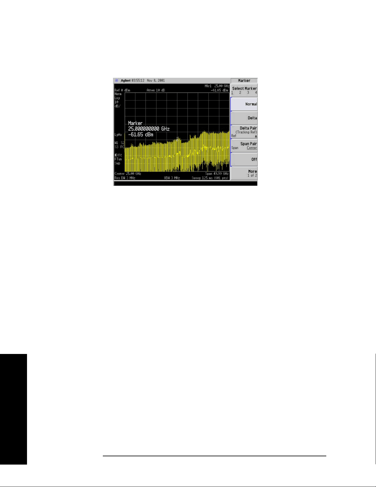
Instrument Functions: A - L

Display

2.5.3.2 Center

Displays the active function in the center-left side of the display.

Key Path:

Display, Active Fctn Position

Readback: Center reads back to line 3 of this key.

State Saved: Not saved in instrument state, survives power cycle and preset.

Factory Preset: No effect, persistent variable, survives power cycle and preset.

Factory Default: Center

History: Added with firmware revision A.04.00

Remote Command:

:DISPlay:AFUNction:POSition CENTer

Example: :DISP:AFUN:POS CENT

Instrument Functions: A - L

100 Chapter 2