

Page 1

Flexible Digital Modulation Analysis
Guide
PSA Series Spectrum Analyzers
Option 241
This manual provides documentation for the following instruments:
Spectrum Analyzers:
E4440A (3 Hz – 26.50 GHz)
E4443A (3 Hz – 6.70 GHz)
E4445A (3 Hz – 13.20 GHz)
E4446A (3 Hz – 44.00 GHz)
E4447A (3 Hz – 42.98 GHz)
E4448A (3 Hz – 50.00 GHz)
Manufacturing Part Number: E4440-90620
Supersedes E4440-90351
Printed in USA
June 2008
© Copyright 1999 - 2008 Agilent Technologies, Inc.
Page 2

Notice
Agilent Technologies makes no warranty of any kind with regard to this
material, including but not limited to, the implied warranties of
merchantability and fitness for a particular purpose. Agilent
Technologies shall not be liable for errors contained herein or for
incidental or consequential damages in connection with the furnishing,
performance, or use of this material.
The information contained in this document is subject to change
without notice.
Additional Information
For the latest information about this analyzer, including firmware
upgrades, application information, and product information, see the
following URL:
http://www.agilent.com/find/psa/
2
Page 3

Contents
1. Introduction
What Does the Agilent PSA Option 241 Do? . . . . . . . . . . . . . . . . . . . . . . . . . . . . . . . . . . . . . . 16
Installing Optional Measurement Personalities . . . . . . . . . . . . . . . . . . . . . . . . . . . . . . . . . . . 18
Do You Have Enough Memory to Load All Your Personality Options? . . . . . . . . . . . . . . . . 18
How to Predict Your Memory Requirements . . . . . . . . . . . . . . . . . . . . . . . . . . . . . . . . . . . . . 20
Loading an Optional Measurement Personality . . . . . . . . . . . . . . . . . . . . . . . . . . . . . . . . . . 22
Obtaining and Installing a License Key . . . . . . . . . . . . . . . . . . . . . . . . . . . . . . . . . . . . . . . . 22
Viewing a License Key . . . . . . . . . . . . . . . . . . . . . . . . . . . . . . . . . . . . . . . . . . . . . . . . . . . . . . 23
Using the Delete License Key on PSA . . . . . . . . . . . . . . . . . . . . . . . . . . . . . . . . . . . . . . . . . . 23
Ordering Optional Measurement Personalities . . . . . . . . . . . . . . . . . . . . . . . . . . . . . . . . . . 24
2. Making Measurements
Introduction . . . . . . . . . . . . . . . . . . . . . . . . . . . . . . . . . . . . . . . . . . . . . . . . . . . . . . . . . . . . . . . . 26
Setting Up the Test Equipment and DUT . . . . . . . . . . . . . . . . . . . . . . . . . . . . . . . . . . . . . . . . 28
Making the Initial Signal Connection . . . . . . . . . . . . . . . . . . . . . . . . . . . . . . . . . . . . . . . . . . 28
Configuring a MS Measurement System. . . . . . . . . . . . . . . . . . . . . . . . . . . . . . . . . . . . . . . . 28
Configuring a BTS Measurement System . . . . . . . . . . . . . . . . . . . . . . . . . . . . . . . . . . . . . . . 29
Using Instrument Presets . . . . . . . . . . . . . . . . . . . . . . . . . . . . . . . . . . . . . . . . . . . . . . . . . . . 30
Determining the RF Parameters of Your Signal . . . . . . . . . . . . . . . . . . . . . . . . . . . . . . . . . . . 31
Using the Spectrum Measurement to View the RF Parameters of the Signal Under Test 31
Spectrum (Frequency Domain) Measurements. . . . . . . . . . . . . . . . . . . . . . . . . . . . . . . . . . . 32
Using the Waveform Measurement to Set Up Triggering (for burst signals) . . . . . . . . . . . 41
Waveform (Time Domain) Measurements . . . . . . . . . . . . . . . . . . . . . . . . . . . . . . . . . . . . . . . 42
Modulation Analysis Measurements in 8 Steps . . . . . . . . . . . . . . . . . . . . . . . . . . . . . . . . . . . . 48
Modulation Analysis Measurement Final Checks . . . . . . . . . . . . . . . . . . . . . . . . . . . . . . . . . . 50
Modifying Measurement Setup Parameters . . . . . . . . . . . . . . . . . . . . . . . . . . . . . . . . . . . . . . . 52
Using the Measurement Setup Form. . . . . . . . . . . . . . . . . . . . . . . . . . . . . . . . . . . . . . . . . . . 52
Setting Demodulation Parameters. . . . . . . . . . . . . . . . . . . . . . . . . . . . . . . . . . . . . . . . . . . . . 53
Setting up a Trigger Source . . . . . . . . . . . . . . . . . . . . . . . . . . . . . . . . . . . . . . . . . . . . . . . . . . 54
Setting Burst/Sync Properties . . . . . . . . . . . . . . . . . . . . . . . . . . . . . . . . . . . . . . . . . . . . . . . . 55
Using Adaptive Equalization . . . . . . . . . . . . . . . . . . . . . . . . . . . . . . . . . . . . . . . . . . . . . . . . . 56
Setting Advanced Measurement Setup Properties . . . . . . . . . . . . . . . . . . . . . . . . . . . . . . . . 59
Measuring Digital Modulation Formats . . . . . . . . . . . . . . . . . . . . . . . . . . . . . . . . . . . . . . . . . . 62
Setting up the Modulation Analysis Personality . . . . . . . . . . . . . . . . . . . . . . . . . . . . . . . . . 63
Viewing the I/Q Polar Vector and Constellation Graphs . . . . . . . . . . . . . . . . . . . . . . . . . . . 64
Viewing the Numeric Measurement Results . . . . . . . . . . . . . . . . . . . . . . . . . . . . . . . . . . . . . 66
Viewing the I/Q Error (Quad-View) Results . . . . . . . . . . . . . . . . . . . . . . . . . . . . . . . . . . . . . 67
Viewing the Magnitude Error Versus Time Results . . . . . . . . . . . . . . . . . . . . . . . . . . . . . . . 68
Viewing the Phase Error Versus Time Results . . . . . . . . . . . . . . . . . . . . . . . . . . . . . . . . . . . 70
Viewing the EVM Versus Time Results . . . . . . . . . . . . . . . . . . . . . . . . . . . . . . . . . . . . . . . . . 73
Viewing the Eye Diagram Results . . . . . . . . . . . . . . . . . . . . . . . . . . . . . . . . . . . . . . . . . . . . . 75
Viewing the FSK Error (Quad-View) Results . . . . . . . . . . . . . . . . . . . . . . . . . . . . . . . . . . . . 77
Viewing the FSK Error Versus Time Results . . . . . . . . . . . . . . . . . . . . . . . . . . . . . . . . . . . . 79
Viewing the FSK Error Spectrum Results. . . . . . . . . . . . . . . . . . . . . . . . . . . . . . . . . . . . . . . 81
Viewing the FSK Measured Time Results . . . . . . . . . . . . . . . . . . . . . . . . . . . . . . . . . . . . . . . 83
PSK Modulation Analysis (cdma2000 QPSK Example) . . . . . . . . . . . . . . . . . . . . . . . . . . . . 85
QAM Modulation Analysis (64QAM Example) . . . . . . . . . . . . . . . . . . . . . . . . . . . . . . . . . . . 87
EDGE Modulation Analysis . . . . . . . . . . . . . . . . . . . . . . . . . . . . . . . . . . . . . . . . . . . . . . . . . 89
FSK Modulation Analysis (Bluetooth 2FSK Example). . . . . . . . . . . . . . . . . . . . . . . . . . . . . 91
Table of Contents
3
Page 4

Contents
Table of Contents
3. Front-Panel Key and SCPI Command Reference
MSK Modulation Analysis (GSM MSK type 1 Example). . . . . . . . . . . . . . . . . . . . . . . . . . . .93
Analyzing and Troubleshooting Digital Signals . . . . . . . . . . . . . . . . . . . . . . . . . . . . . . . . . . . .95
EVM Troubleshooting Procedure Overview . . . . . . . . . . . . . . . . . . . . . . . . . . . . . . . . . . . . . .95
Measurement 1 - Obtaining EVM Results with Phase Error and Magnitude Error . . . . . .96
Measurement 2 - Phase Error vs. Time . . . . . . . . . . . . . . . . . . . . . . . . . . . . . . . . . . . . . . . . .97
Measurement 3 - Magnitude Error vs. Time . . . . . . . . . . . . . . . . . . . . . . . . . . . . . . . . . . . . .98
Measurement 4 - I/Q Constellation Diagram . . . . . . . . . . . . . . . . . . . . . . . . . . . . . . . . . . . . .99
Measurement 5 - Error Vector Magnitude vs. Time. . . . . . . . . . . . . . . . . . . . . . . . . . . . . . .101
Interpreting Measurement Results (Impairments) . . . . . . . . . . . . . . . . . . . . . . . . . . . . . . .102
SCPI Programming a Modulation Measurement . . . . . . . . . . . . . . . . . . . . . . . . . . . . . . . . . . 118
Interpreting Error Codes . . . . . . . . . . . . . . . . . . . . . . . . . . . . . . . . . . . . . . . . . . . . . . . . . . . . .119
Instrument Front Panel Highlights . . . . . . . . . . . . . . . . . . . . . . . . . . . . . . . . . . . . . . . . . . . . .122
Selected PSA Front-Panel Features . . . . . . . . . . . . . . . . . . . . . . . . . . . . . . . . . . . . . . . . . . .123
Front-Panel Keys . . . . . . . . . . . . . . . . . . . . . . . . . . . . . . . . . . . . . . . . . . . . . . . . . . . . . . . . . . . .124
Det/Demod . . . . . . . . . . . . . . . . . . . . . . . . . . . . . . . . . . . . . . . . . . . . . . . . . . . . . . . . . . . . . . .124
FREQUENCY Channel . . . . . . . . . . . . . . . . . . . . . . . . . . . . . . . . . . . . . . . . . . . . . . . . . . . . .124
Input/Output. . . . . . . . . . . . . . . . . . . . . . . . . . . . . . . . . . . . . . . . . . . . . . . . . . . . . . . . . . . . . .126
Meas Control. . . . . . . . . . . . . . . . . . . . . . . . . . . . . . . . . . . . . . . . . . . . . . . . . . . . . . . . . . . . . .129
MEASURE . . . . . . . . . . . . . . . . . . . . . . . . . . . . . . . . . . . . . . . . . . . . . . . . . . . . . . . . . . . . . . .130
Mode . . . . . . . . . . . . . . . . . . . . . . . . . . . . . . . . . . . . . . . . . . . . . . . . . . . . . . . . . . . . . . . . . . . .130
Instrument Selection by Name (Remote command only). . . . . . . . . . . . . . . . . . . . . . . . . . .131
Instrument Selection by Number (Remote command only) . . . . . . . . . . . . . . . . . . . . . . . . .131
Mode Setup . . . . . . . . . . . . . . . . . . . . . . . . . . . . . . . . . . . . . . . . . . . . . . . . . . . . . . . . . . . . . . .131
Trig . . . . . . . . . . . . . . . . . . . . . . . . . . . . . . . . . . . . . . . . . . . . . . . . . . . . . . . . . . . . . . . . . . . . .133
Modulation Analysis Measurement Keys . . . . . . . . . . . . . . . . . . . . . . . . . . . . . . . . . . . . . . . .141
AMPLITUDE Y Scale. . . . . . . . . . . . . . . . . . . . . . . . . . . . . . . . . . . . . . . . . . . . . . . . . . . . . . .141
Y Scale / Div . . . . . . . . . . . . . . . . . . . . . . . . . . . . . . . . . . . . . . . . . . . . . . . . . . . . . . . . . . . . . .142
Y Ref Value . . . . . . . . . . . . . . . . . . . . . . . . . . . . . . . . . . . . . . . . . . . . . . . . . . . . . . . . . . . . . . .143
Y Ref Position . . . . . . . . . . . . . . . . . . . . . . . . . . . . . . . . . . . . . . . . . . . . . . . . . . . . . . . . . . . . .143
Y Scale Coupling. . . . . . . . . . . . . . . . . . . . . . . . . . . . . . . . . . . . . . . . . . . . . . . . . . . . . . . . . . .144
Display . . . . . . . . . . . . . . . . . . . . . . . . . . . . . . . . . . . . . . . . . . . . . . . . . . . . . . . . . . . . . . . . . .144
Markers. . . . . . . . . . . . . . . . . . . . . . . . . . . . . . . . . . . . . . . . . . . . . . . . . . . . . . . . . . . . . . . . . .148
Meas Setup . . . . . . . . . . . . . . . . . . . . . . . . . . . . . . . . . . . . . . . . . . . . . . . . . . . . . . . . . . . . . . .150
SPAN X Scale . . . . . . . . . . . . . . . . . . . . . . . . . . . . . . . . . . . . . . . . . . . . . . . . . . . . . . . . . . . . .176
Trace/View. . . . . . . . . . . . . . . . . . . . . . . . . . . . . . . . . . . . . . . . . . . . . . . . . . . . . . . . . . . . . . . .179
SCPI only operations . . . . . . . . . . . . . . . . . . . . . . . . . . . . . . . . . . . . . . . . . . . . . . . . . . . . . . . . .180
Trig Error Offset. . . . . . . . . . . . . . . . . . . . . . . . . . . . . . . . . . . . . . . . . . . . . . . . . . . . . . . . . . .180
SCPI Result Table . . . . . . . . . . . . . . . . . . . . . . . . . . . . . . . . . . . . . . . . . . . . . . . . . . . . . . . . .180
Averaging . . . . . . . . . . . . . . . . . . . . . . . . . . . . . . . . . . . . . . . . . . . . . . . . . . . . . . . . . . . . . . . .187
4. Concepts
Introduction . . . . . . . . . . . . . . . . . . . . . . . . . . . . . . . . . . . . . . . . . . . . . . . . . . . . . . . . . . . . . . . .190
Introduction to Digital Modulation . . . . . . . . . . . . . . . . . . . . . . . . . . . . . . . . . . . . . . . . . . . . .191
Why Choose Digital Instead of Analog Modulation? . . . . . . . . . . . . . . . . . . . . . . . . . . . . . .191
What is Digital Modulation? . . . . . . . . . . . . . . . . . . . . . . . . . . . . . . . . . . . . . . . . . . . . . . . . .191
PSK examples . . . . . . . . . . . . . . . . . . . . . . . . . . . . . . . . . . . . . . . . . . . . . . . . . . . . . . . . . . . .194
4
Page 5

Contents
Orthogonality . . . . . . . . . . . . . . . . . . . . . . . . . . . . . . . . . . . . . . . . . . . . . . . . . . . . . . . . . . . . 195
QAM example . . . . . . . . . . . . . . . . . . . . . . . . . . . . . . . . . . . . . . . . . . . . . . . . . . . . . . . . . . . . 195
Symbol Rate. . . . . . . . . . . . . . . . . . . . . . . . . . . . . . . . . . . . . . . . . . . . . . . . . . . . . . . . . . . . . . 196
Bandwidth . . . . . . . . . . . . . . . . . . . . . . . . . . . . . . . . . . . . . . . . . . . . . . . . . . . . . . . . . . . . . . . 196
Filtering . . . . . . . . . . . . . . . . . . . . . . . . . . . . . . . . . . . . . . . . . . . . . . . . . . . . . . . . . . . . . . . . . 197
Effects Of Going Through The Origin . . . . . . . . . . . . . . . . . . . . . . . . . . . . . . . . . . . . . . . . . 199
Transmitting the Digital Signal . . . . . . . . . . . . . . . . . . . . . . . . . . . . . . . . . . . . . . . . . . . . . . 200
I/Q Modulator . . . . . . . . . . . . . . . . . . . . . . . . . . . . . . . . . . . . . . . . . . . . . . . . . . . . . . . . . . . . 200
System Multiplexing . . . . . . . . . . . . . . . . . . . . . . . . . . . . . . . . . . . . . . . . . . . . . . . . . . . . . . . 201
Digital Modulation Format Standards . . . . . . . . . . . . . . . . . . . . . . . . . . . . . . . . . . . . . . . . . . 203
Introduction. . . . . . . . . . . . . . . . . . . . . . . . . . . . . . . . . . . . . . . . . . . . . . . . . . . . . . . . . . . . . . 203
Modulation Formats and Applications . . . . . . . . . . . . . . . . . . . . . . . . . . . . . . . . . . . . . . . . 203
Families of Format and data sheets. . . . . . . . . . . . . . . . . . . . . . . . . . . . . . . . . . . . . . . . . . . 203
Applications . . . . . . . . . . . . . . . . . . . . . . . . . . . . . . . . . . . . . . . . . . . . . . . . . . . . . . . . . . . . . . 204
Phase Shift Keying (PSK) Concepts. . . . . . . . . . . . . . . . . . . . . . . . . . . . . . . . . . . . . . . . . . . 205
Frequency Shift Keying (FSK) Concepts . . . . . . . . . . . . . . . . . . . . . . . . . . . . . . . . . . . . . . . 215
Minimum Shift Keying (MSK) Concepts . . . . . . . . . . . . . . . . . . . . . . . . . . . . . . . . . . . . . . . 218
Quadrature Amplitude Modulation (QAM) Concepts . . . . . . . . . . . . . . . . . . . . . . . . . . . . . 221
Modulation Bit State Diagrams . . . . . . . . . . . . . . . . . . . . . . . . . . . . . . . . . . . . . . . . . . . . . . 224
Communication System Formats . . . . . . . . . . . . . . . . . . . . . . . . . . . . . . . . . . . . . . . . . . . . . . 238
PSA option 241 Communications Format Standards . . . . . . . . . . . . . . . . . . . . . . . . . . . . . 238
What is the cdmaOne (IS-95) Communication System? . . . . . . . . . . . . . . . . . . . . . . . . . . . 239
cdmaOne Communication System . . . . . . . . . . . . . . . . . . . . . . . . . . . . . . . . . . . . . . . . . . . . 241
What is the W-CDMA Communications System? . . . . . . . . . . . . . . . . . . . . . . . . . . . . . . . . 242
W-CDMA Communication System . . . . . . . . . . . . . . . . . . . . . . . . . . . . . . . . . . . . . . . . . . . . 246
What Is the cdma2000 Communication System? . . . . . . . . . . . . . . . . . . . . . . . . . . . . . . . . 247
cdma2000 Communication System . . . . . . . . . . . . . . . . . . . . . . . . . . . . . . . . . . . . . . . . . . . 250
What is the NADC Communications System? . . . . . . . . . . . . . . . . . . . . . . . . . . . . . . . . . . 251
NADC Communication System . . . . . . . . . . . . . . . . . . . . . . . . . . . . . . . . . . . . . . . . . . . . . . 254
What is the PDC Communications System? . . . . . . . . . . . . . . . . . . . . . . . . . . . . . . . . . . . . 255
PDC Communication System . . . . . . . . . . . . . . . . . . . . . . . . . . . . . . . . . . . . . . . . . . . . . . . . 256
What is the PHS Communication System . . . . . . . . . . . . . . . . . . . . . . . . . . . . . . . . . . . . . . 257
PHS Communication System . . . . . . . . . . . . . . . . . . . . . . . . . . . . . . . . . . . . . . . . . . . . . . . . 258
What is the TETRA Communications System . . . . . . . . . . . . . . . . . . . . . . . . . . . . . . . . . . 259
TETRA Communication System . . . . . . . . . . . . . . . . . . . . . . . . . . . . . . . . . . . . . . . . . . . . . 261
What is Bluetooth? . . . . . . . . . . . . . . . . . . . . . . . . . . . . . . . . . . . . . . . . . . . . . . . . . . . . . . . . 262
Bluetooth Communication System. . . . . . . . . . . . . . . . . . . . . . . . . . . . . . . . . . . . . . . . . . . . 265
What are GSM and EDGE? . . . . . . . . . . . . . . . . . . . . . . . . . . . . . . . . . . . . . . . . . . . . . . . . . 266
EDGE Communication System . . . . . . . . . . . . . . . . . . . . . . . . . . . . . . . . . . . . . . . . . . . . . . 270
What is APCO25 phase 1? . . . . . . . . . . . . . . . . . . . . . . . . . . . . . . . . . . . . . . . . . . . . . . . . . . 271
APCO25 phase1 Communication System . . . . . . . . . . . . . . . . . . . . . . . . . . . . . . . . . . . . . . 275
What is VDL Mode 3? . . . . . . . . . . . . . . . . . . . . . . . . . . . . . . . . . . . . . . . . . . . . . . . . . . . . . . 276
What is ZigBee (IEEE 802.15.4)? . . . . . . . . . . . . . . . . . . . . . . . . . . . . . . . . . . . . . . . . . . . . . 277
Measurements on Digital RF Communications Systems. . . . . . . . . . . . . . . . . . . . . . . . . . . . 278
Introduction. . . . . . . . . . . . . . . . . . . . . . . . . . . . . . . . . . . . . . . . . . . . . . . . . . . . . . . . . . . . . . 278
Digital Modulation Analysis . . . . . . . . . . . . . . . . . . . . . . . . . . . . . . . . . . . . . . . . . . . . . . . . 278
Measurement Domains . . . . . . . . . . . . . . . . . . . . . . . . . . . . . . . . . . . . . . . . . . . . . . . . . . . . . 279
PSA Digital Demodulator . . . . . . . . . . . . . . . . . . . . . . . . . . . . . . . . . . . . . . . . . . . . . . . . . . 281
Modulation quality measurements . . . . . . . . . . . . . . . . . . . . . . . . . . . . . . . . . . . . . . . . . . . 286
Table of Contents
5
Page 6

Contents
Table of Contents
5. Menu Maps
Digital Modulation Errors and Signal Impairments . . . . . . . . . . . . . . . . . . . . . . . . . . . . . .292
Impairments . . . . . . . . . . . . . . . . . . . . . . . . . . . . . . . . . . . . . . . . . . . . . . . . . . . . . . . . . . . . . .295
Digital Modulation Displays . . . . . . . . . . . . . . . . . . . . . . . . . . . . . . . . . . . . . . . . . . . . . . . . .300
References . . . . . . . . . . . . . . . . . . . . . . . . . . . . . . . . . . . . . . . . . . . . . . . . . . . . . . . . . . . . . . . . .308
Other Sources of Digital Modulation Information . . . . . . . . . . . . . . . . . . . . . . . . . . . . . . . .308
Flexible Digital Modulation Analysis Key Flow . . . . . . . . . . . . . . . . . . . . . . . . . . . . . . . . . . .310
Directions for Use . . . . . . . . . . . . . . . . . . . . . . . . . . . . . . . . . . . . . . . . . . . . . . . . . . . . . . . . . 311
6
Page 7

List of Commands
:CALCulate:<measurement>:MARKer[1]|2|3|4:TRACe EVM
|MERRor|PERRor|EIRReal|EIRImag|ECRMagnitude|ECRPhase
|EVSPectrum|AEVSpectrum|FERRor|FESPectrum|AFESpectrum
|FMEAsured|DBITs|RFSPectrum|ARFSpectrum . . . . . . . . . . . . . . . . . . . . . . . . . . . . . . . . . . . . 150
:CALCulate:<measurement>:MARKer[1]|2|3|4:TRACe? . . . . . . . . . . . . . . . . . . . . . . . . . . . . . . . 150
:CALCulate:EVM:LIMit:FERRor <frequency> . . . . . . . . . . . . . . . . . . . . . . . . . . . . . . . . . . . . . . . . . 167
:CALCulate:EVM:LIMit:FERRor:STATe ON|OFF|1|0 . . . . . . . . . . . . . . . . . . . . . . . . . . . . . . . . . 167
:CALCulate:EVM:LIMit:FERRor:STATe? . . . . . . . . . . . . . . . . . . . . . . . . . . . . . . . . . . . . . . . . . . . . . 167
:CALCulate:EVM:LIMit:FERRor? . . . . . . . . . . . . . . . . . . . . . . . . . . . . . . . . . . . . . . . . . . . . . . . . . . . 167
:CALCulate:EVM:LIMit:RMS <real> . . . . . . . . . . . . . . . . . . . . . . . . . . . . . . . . . . . . . . . . . . . . . . . . 167
:CALCulate:EVM:LIMit:RMS:STATe ON|OFF|1|0 . . . . . . . . . . . . . . . . . . . . . . . . . . . . . . . . . . . . 167
:CALCulate:EVM:LIMit:RMS:STATe?. . . . . . . . . . . . . . . . . . . . . . . . . . . . . . . . . . . . . . . . . . . . . . . . 167
:CALCulate:EVM:LIMit:RMS? . . . . . . . . . . . . . . . . . . . . . . . . . . . . . . . . . . . . . . . . . . . . . . . . . . . . . 167
:CALCulate:EVM:MARKer[1]|2|3|4:FUNCtion BPOWer|NOISe|OFF . . . . . . . . . . . . . . . . . . . 149
:CALCulate:EVM:MARKer[1]|2|3|4:FUNCtion? . . . . . . . . . . . . . . . . . . . . . . . . . . . . . . . . . . . . . . 149
:CALCulate:EVM:MARKer[1]|2|3|4[:STATe] OFF|ON|0|1 . . . . . . . . . . . . . . . . . . . . . . . . . . . . 150
:CONFigure:EVM . . . . . . . . . . . . . . . . . . . . . . . . . . . . . . . . . . . . . . . . . . . . . . . . . . . . . . . . . . . . . . . . 180
:DISPlay:EVM:FVECtor[:STATe] OFF|ON|0|1 . . . . . . . . . . . . . . . . . . . . . . . . . . . . . . . . . . . . . . . 145
:DISPlay:EVM:FVECtor[:STATe]? . . . . . . . . . . . . . . . . . . . . . . . . . . . . . . . . . . . . . . . . . . . . . . . . . . . 145
:DISPlay:EVM:IQPoints <integer> . . . . . . . . . . . . . . . . . . . . . . . . . . . . . . . . . . . . . . . . . . . . . . . . . . 144
:DISPlay:EVM:IQPoints:OFFSet <integer> . . . . . . . . . . . . . . . . . . . . . . . . . . . . . . . . . . . . . . . . . . . 145
:DISPlay:EVM:IQPoints:OFFSet? . . . . . . . . . . . . . . . . . . . . . . . . . . . . . . . . . . . . . . . . . . . . . . . . . . . 145
:DISPlay:EVM:IQPoints? . . . . . . . . . . . . . . . . . . . . . . . . . . . . . . . . . . . . . . . . . . . . . . . . . . . . . . . . . . 144
List of Commands
:DISPlay:EVM:IQPType VCONstln|VECTor|CONStln . . . . . . . . . . . . . . . . . . . . . . . . . . . . . . . . . 146
:DISPlay:EVM:IQPType? . . . . . . . . . . . . . . . . . . . . . . . . . . . . . . . . . . . . . . . . . . . . . . . . . . . . . . . . . . 146
:DISPlay:EVM:IQRotation <degree> . . . . . . . . . . . . . . . . . . . . . . . . . . . . . . . . . . . . . . . . . . . . . . . . . 147
:DISPlay:EVM:IQRotation:STATe ON|OFF|1|0. . . . . . . . . . . . . . . . . . . . . . . . . . . . . . . . . . . . . . . 147
:DISPlay:EVM:IQRotation:STATe? . . . . . . . . . . . . . . . . . . . . . . . . . . . . . . . . . . . . . . . . . . . . . . . . . . 147
:DISPlay:EVM:IQRotation? . . . . . . . . . . . . . . . . . . . . . . . . . . . . . . . . . . . . . . . . . . . . . . . . . . . . . . . . 147
:DISPlay:EVM:PPSYmbol ONE|TWO|FOUR|FIVE|TEN . . . . . . . . . . . . . . . . . . . . . . . . . . . . . . 146
:DISPlay:EVM:PPSYmbol? . . . . . . . . . . . . . . . . . . . . . . . . . . . . . . . . . . . . . . . . . . . . . . . . . . . . . . . . 146
:DISPlay:EVM:VIEW POLar|IQERror|EYE|FSKError|NRESults
7
Page 8

List of Commands
List of Commands
|DBITs|EVSPectum|EQUalizer . . . . . . . . . . . . . . . . . . . . . . . . . . . . . . . . . . . . . . . . . . . . . . . . . . . .179
:DISPlay:EVM:VIEW? . . . . . . . . . . . . . . . . . . . . . . . . . . . . . . . . . . . . . . . . . . . . . . . . . . . . . . . . . . . . .179
:DISPlay:EVM[1]|2|3|4|5|6|7|8:WINDow[1]|2|3|4:TRACe:
X[:SCALe]:COUPle OFF|ON|0|1 . . . . . . . . . . . . . . . . . . . . . . . . . . . . . . . . . . . . . . . . . . . . . . . . . . .178
:DISPlay:EVM[1]|2|3|4|5|6|7|8:WINDow[1]|2|3|4:TRACe:X[:SCALe]:COUPle? . . . . . . . . . .178
:DISPlay:EVM[1]|2|3|4|5|6|7|8:WINDow[1]|2|3|4:
TRACe:X[:SCALe]:PDIVision <real> . . . . . . . . . . . . . . . . . . . . . . . . . . . . . . . . . . . . . . . . . . . . . . . . .177
:DISPlay:EVM[1]|2|3|4|5|6|7|8:WINDow[1]|2|3|4:TRACe:X[:SCALe]:PDIVision? . . . . . . . .177
:DISPlay:EVM[1]|2|3|4|5|6|7|8:WINDow[1]|2|3|4:TRACe:X[:SCALe]:RLEVel <real> . . . . .177
:DISPlay:EVM[1]|2|3|4|5|6|7|8:WINDow[1]|2|3|4:TRACe:X[:SCALe]:RLEVel? . . . . . . . . . .177
:DISPlay:EVM[1]|2|3|4|5|6|7|8:WINDow[1]|2|3|4:
TRACe:X[:SCALe]:RPOSition LEFT|CENTer|RIGHt . . . . . . . . . . . . . . . . . . . . . . . . . . . . . . . . . . .178
:DISPlay:EVM[1]|2|3|4|5|6|7|8:WINDow[1]|2|3|4:TRACe:X[:SCALe]:RPOSition? . . . . . . . .178
:DISPlay:EVM[1]|2|3|4|5|6|7|8:WINDow[1]|2|3|4:TRACe:
Y[:SCALe]:COUPle 0|1|OFF|ON . . . . . . . . . . . . . . . . . . . . . . . . . . . . . . . . . . . . . . . . . . . . . . . . . . .144
:DISPlay:EVM[1]|2|3|4|5|6|7|8:WINDow[1]|2|3|4:TRACe:Y[:SCALe]:COUPle? . . . . . . . . . .144
:DISPlay:EVM[1]|2|3|4|5|6|7|8:WINDow[1]|2|3|4:TRACe:Y[:SCALe]:PDIVision <real> . . .142
:DISPlay:EVM[1]|2|3|4|5|6|7|8:WINDow[1]|2|3|4:TRACe:Y[:SCALe]:PDIVision? . . . . . . . .142
:DISPlay:EVM[1]|2|3|4|5|6|7|8:WINDow[1]|2|3|4:TRACe:Y[:SCALe]:RLEVel <real> . . . . .143
:DISPlay:EVM[1]|2|3|4|5|6|7|8:WINDow[1]|2|3|4:TRACe:Y[:SCALe]:RLEVel? . . . . . . . . . .143
:DISPlay:EVM[1]|2|3|4|5|6|7|8:WINDow[1]|2|3|4:TRACe:
Y[:SCALe]:RPOSition TOP|CENTer|BOTTom. . . . . . . . . . . . . . . . . . . . . . . . . . . . . . . . . . . . . . . . .143
:DISPlay:EVM[1]|2|3|4|5|6|7|8:WINDow[1]|2|3|4:TRACe:Y[:SCALe]:
RPOSition? . . . . . . . . . . . . . . . . . . . . . . . . . . . . . . . . . . . . . . . . . . . . . . . . . . . . . . . . . . . . . . . . . . . . . .143
:FETCh:EVM[n]? . . . . . . . . . . . . . . . . . . . . . . . . . . . . . . . . . . . . . . . . . . . . . . . . . . . . . . . . . . . . . . . . .180
:INITiate:CONTinuous OFF|ON . . . . . . . . . . . . . . . . . . . . . . . . . . . . . . . . . . . . . . . . . . . . . . . . . . . .129
:INITiate:EVM . . . . . . . . . . . . . . . . . . . . . . . . . . . . . . . . . . . . . . . . . . . . . . . . . . . . . . . . . . . . . . . . . . .180
:INITiate:PAUSe . . . . . . . . . . . . . . . . . . . . . . . . . . . . . . . . . . . . . . . . . . . . . . . . . . . . . . . . . . . . . . . . .130
:INITiate:RESTart . . . . . . . . . . . . . . . . . . . . . . . . . . . . . . . . . . . . . . . . . . . . . . . . . . . . . . . . . . . . . . . .129
:INITiate:RESume . . . . . . . . . . . . . . . . . . . . . . . . . . . . . . . . . . . . . . . . . . . . . . . . . . . . . . . . . . . . . . . .130
:INSTrument:NSELect 241 . . . . . . . . . . . . . . . . . . . . . . . . . . . . . . . . . . . . . . . . . . . . . . . . . . . . . . . . .131
:INSTrument:NSELect?. . . . . . . . . . . . . . . . . . . . . . . . . . . . . . . . . . . . . . . . . . . . . . . . . . . . . . . . . . . .131
:INSTrument[:SELect] SA|BASIC|DMODULATION . . . . . . . . . . . . . . . . . . . . . . . . . . . . . . . . . . .131
8
Page 9

List of Commands
:INSTrument[:SELect]? . . . . . . . . . . . . . . . . . . . . . . . . . . . . . . . . . . . . . . . . . . . . . . . . . . . . . . . . . . . 131
:MEASure:EVM[n]? . . . . . . . . . . . . . . . . . . . . . . . . . . . . . . . . . . . . . . . . . . . . . . . . . . . . . . . . . . . . . . 180
:READ:EVM[n]? . . . . . . . . . . . . . . . . . . . . . . . . . . . . . . . . . . . . . . . . . . . . . . . . . . . . . . . . . . . . . . . . . 180
:TRIGger[:SEQuence]:AUTO:STATe ON|OFF|1|0. . . . . . . . . . . . . . . . . . . . . . . . . . . . . . . . . . . . . 138
:TRIGger[:SEQuence]:AUTO:STATe? . . . . . . . . . . . . . . . . . . . . . . . . . . . . . . . . . . . . . . . . . . . . . . . . 138
:TRIGger[:SEQuence]:AUTO[:TIME] <time> . . . . . . . . . . . . . . . . . . . . . . . . . . . . . . . . . . . . . . . . . . 138
:TRIGger[:SEQuence]:AUTO[:TIME]?. . . . . . . . . . . . . . . . . . . . . . . . . . . . . . . . . . . . . . . . . . . . . . . . 138
:TRIGger[:SEQuence]:EXTernal[1]|2:DELay <time> . . . . . . . . . . . . . . . . . . . . . . . . . . . . . . . . . . . 136
:TRIGger[:SEQuence]:EXTernal[1]|2:DELay? . . . . . . . . . . . . . . . . . . . . . . . . . . . . . . . . . . . . . . . . . 136
:TRIGger[:SEQuence]:EXTernal[1]|2:LEVel <voltage> . . . . . . . . . . . . . . . . . . . . . . . . . . . . . . . . . . 137
List of Commands
:TRIGger[:SEQuence]:EXTernal[1]|2:LEVel?. . . . . . . . . . . . . . . . . . . . . . . . . . . . . . . . . . . . . . . . . . 137
:TRIGger[:SEQuence]:EXTernal[1]|2:SLOPe NEGative|POSitive . . . . . . . . . . . . . . . . . . . . . . . . 137
:TRIGger[:SEQuence]:EXTernal[1]|2:SLOPe? . . . . . . . . . . . . . . . . . . . . . . . . . . . . . . . . . . . . . . . . . 137
:TRIGger[:SEQuence]:FRAMe:PERiod <time> . . . . . . . . . . . . . . . . . . . . . . . . . . . . . . . . . . . . . . . . . 139
:TRIGger[:SEQuence]:FRAMe:PERiod? . . . . . . . . . . . . . . . . . . . . . . . . . . . . . . . . . . . . . . . . . . . . . . 139
:TRIGger[:SEQuence]:FRAMe:SYNCmode OFF|EXTFront|EXTRear . . . . . . . . . . . . . . . . . . . . . 140
:TRIGger[:SEQuence]:FRAMe:SYNCmode:OFFSet <time> . . . . . . . . . . . . . . . . . . . . . . . . . . . . . . 139
:TRIGger[:SEQuence]:FRAMe:SYNCmode:OFFSet? . . . . . . . . . . . . . . . . . . . . . . . . . . . . . . . . . . . . 139
:TRIGger[:SEQuence]:FRAMe:SYNCmode? . . . . . . . . . . . . . . . . . . . . . . . . . . . . . . . . . . . . . . . . . . . 140
:TRIGger[:SEQuence]:HOLDoff <time> . . . . . . . . . . . . . . . . . . . . . . . . . . . . . . . . . . . . . . . . . . . . . . 138
:TRIGger[:SEQuence]:HOLDoff? . . . . . . . . . . . . . . . . . . . . . . . . . . . . . . . . . . . . . . . . . . . . . . . . . . . . 138
:TRIGger[:SEQuence]:IF:DELay <time>. . . . . . . . . . . . . . . . . . . . . . . . . . . . . . . . . . . . . . . . . . . . . . 135
:TRIGger[:SEQuence]:IF:DELay? . . . . . . . . . . . . . . . . . . . . . . . . . . . . . . . . . . . . . . . . . . . . . . . . . . . 135
:TRIGger[:SEQuence]:IF:LEVel <ampl> . . . . . . . . . . . . . . . . . . . . . . . . . . . . . . . . . . . . . . . . . . . . . . 135
:TRIGger[:SEQuence]:IF:LEVel? . . . . . . . . . . . . . . . . . . . . . . . . . . . . . . . . . . . . . . . . . . . . . . . . . . . . 135
:TRIGger[:SEQuence]:IF:SLOPe NEGative|POSitive . . . . . . . . . . . . . . . . . . . . . . . . . . . . . . . . . . . 136
:TRIGger[:SEQuence]:IF:SLOPe? . . . . . . . . . . . . . . . . . . . . . . . . . . . . . . . . . . . . . . . . . . . . . . . . . . . 136
:TRIGger[:SEQuence]:RFBurst:DELay <time> . . . . . . . . . . . . . . . . . . . . . . . . . . . . . . . . . . . . . . . . 134
:TRIGger[:SEQuence]:RFBurst:DELay? . . . . . . . . . . . . . . . . . . . . . . . . . . . . . . . . . . . . . . . . . . . . . . 134
:TRIGger[:SEQuence]:RFBurst:LEVel <rel_power>. . . . . . . . . . . . . . . . . . . . . . . . . . . . . . . . . . . . . 134
:TRIGger[:SEQuence]:RFBurst:LEVel?. . . . . . . . . . . . . . . . . . . . . . . . . . . . . . . . . . . . . . . . . . . . . . . 134
9
Page 10

List of Commands
:TRIGger[:SEQuence]:RFBurst:SLOPe NEGative|POSitive . . . . . . . . . . . . . . . . . . . . . . . . . . . . . .135
:TRIGger[:SEQuence]:RFBurst:SLOPe?. . . . . . . . . . . . . . . . . . . . . . . . . . . . . . . . . . . . . . . . . . . . . . .135
[:SENSe]:CORRection:BTS:[:RF]:LOSS <real> . . . . . . . . . . . . . . . . . . . . . . . . . . . . . . . . . . . . . . . . .128
[:SENSe]:CORRection:BTS:[:RF]:LOSS? . . . . . . . . . . . . . . . . . . . . . . . . . . . . . . . . . . . . . . . . . . . . . .128
[:SENSe]:CORRection:MS:[:RF]:LOSS <real> . . . . . . . . . . . . . . . . . . . . . . . . . . . . . . . . . . . . . . . . . .128
[:SENSe]:CORRection:MS:[:RF]:LOSS? . . . . . . . . . . . . . . . . . . . . . . . . . . . . . . . . . . . . . . . . . . . . . . .128
[:SENSe]:EVM:ADC:RANGe AUTO|NONE|Autopeaklock|ENVL|0dB|6dB|12dB|18dB. . . . .170
[:SENSe]:EVM:ADC:RANGe? . . . . . . . . . . . . . . . . . . . . . . . . . . . . . . . . . . . . . . . . . . . . . . . . . . . . . . .170
[:SENSe]:EVM:ADRoop:COMPensation ON|OFF|0|1 . . . . . . . . . . . . . . . . . . . . . . . . . . . . . . . . . .174
[:SENSe]:EVM:ADRoop:COMPensation? . . . . . . . . . . . . . . . . . . . . . . . . . . . . . . . . . . . . . . . . . . . . . .174
List of Commands
[:SENSe]:EVM:AVERage:COUNt <integer> . . . . . . . . . . . . . . . . . . . . . . . . . . . . . . . . . . . . . . . . . . .151
[:SENSe]:EVM:AVERage:COUNt? . . . . . . . . . . . . . . . . . . . . . . . . . . . . . . . . . . . . . . . . . . . . . . . . . . .151
[:SENSe]:EVM:AVERage:TCONtrol EXPonential|REPeat . . . . . . . . . . . . . . . . . . . . . . . . . . . . . . .152
[:SENSe]:EVM:AVERage:TCONtrol? . . . . . . . . . . . . . . . . . . . . . . . . . . . . . . . . . . . . . . . . . . . . . . . . .152
[:SENSe]:EVM:AVERage:TRACe[:TYPE] RMS|MAXimum|MINimum . . . . . . . . . . . . . . . . . . . . .153
[:SENSe]:EVM:AVERage:TRACe[:TYPE]? . . . . . . . . . . . . . . . . . . . . . . . . . . . . . . . . . . . . . . . . . . . . .153
[:SENSe]:EVM:AVERage[:STATe] OFF|ON|0|1 . . . . . . . . . . . . . . . . . . . . . . . . . . . . . . . . . . . . . . .151
[:SENSe]:EVM:AVERage[:STATe]? . . . . . . . . . . . . . . . . . . . . . . . . . . . . . . . . . . . . . . . . . . . . . . . . . . .151
[:SENSe]:EVM:CADJust <real> . . . . . . . . . . . . . . . . . . . . . . . . . . . . . . . . . . . . . . . . . . . . . . . . . . . . .168
[:SENSe]:EVM:CADJust? . . . . . . . . . . . . . . . . . . . . . . . . . . . . . . . . . . . . . . . . . . . . . . . . . . . . . . . . . .168
[:SENSe]:EVM:CLOCk NORMal|WIDE . . . . . . . . . . . . . . . . . . . . . . . . . . . . . . . . . . . . . . . . . . . . . .165
[:SENSe]:EVM:CLOCk:WIDE:AUTO ON|OFF|0|1 . . . . . . . . . . . . . . . . . . . . . . . . . . . . . . . . . . . .173
[:SENSe]:EVM:CLOCk:WIDE:AUTO? . . . . . . . . . . . . . . . . . . . . . . . . . . . . . . . . . . . . . . . . . . . . . . . .173
[:SENSe]:EVM:CLOCk:WIDE:MRANge <freq>. . . . . . . . . . . . . . . . . . . . . . . . . . . . . . . . . . . . . . . . .174
[:SENSe]:EVM:CLOCk:WIDE:MRANge? . . . . . . . . . . . . . . . . . . . . . . . . . . . . . . . . . . . . . . . . . . . . . .174
[:SENSe]:EVM:CLOCk?. . . . . . . . . . . . . . . . . . . . . . . . . . . . . . . . . . . . . . . . . . . . . . . . . . . . . . . . . . . .165
[:SENSe]:EVM:CMODe RMS| MAXimum. . . . . . . . . . . . . . . . . . . . . . . . . . . . . . . . . . . . . . . . . . . . .169
[:SENSe]:EVM:CMODe? . . . . . . . . . . . . . . . . . . . . . . . . . . . . . . . . . . . . . . . . . . . . . . . . . . . . . . . . . . .169
[:SENSe]:EVM:EQUalization:CONVergence <real> . . . . . . . . . . . . . . . . . . . . . . . . . . . . . . . . . . . . .164
[:SENSe]:EVM:EQUalization:CONVergence? . . . . . . . . . . . . . . . . . . . . . . . . . . . . . . . . . . . . . . . . . .164
[:SENSe]:EVM:EQUalization:FLENgth <integer> . . . . . . . . . . . . . . . . . . . . . . . . . . . . . . . . . . . . . .163
10
Page 11

List of Commands
[:SENSe]:EVM:EQUalization:FLENgth? . . . . . . . . . . . . . . . . . . . . . . . . . . . . . . . . . . . . . . . . . . . . . 163
[:SENSe]:EVM:EQUalization:HOLD[:STATe] OFF|ON|0|1 . . . . . . . . . . . . . . . . . . . . . . . . . . . . . 164
[:SENSe]:EVM:EQUalization:HOLD[:STATe]?. . . . . . . . . . . . . . . . . . . . . . . . . . . . . . . . . . . . . . . . . 164
[:SENSe]:EVM:EQUalization:RESet . . . . . . . . . . . . . . . . . . . . . . . . . . . . . . . . . . . . . . . . . . . . . . . . . 165
[:SENSe]:EVM:EQUalization[:STATe] OFF|ON|0|1 . . . . . . . . . . . . . . . . . . . . . . . . . . . . . . . . . . . 163
[:SENSe]:EVM:EQUalization[:STATe]?. . . . . . . . . . . . . . . . . . . . . . . . . . . . . . . . . . . . . . . . . . . . . . . 163
[:SENSe]:EVM:FFT:WINDow[:TYPE] UNIForm|FTOP|HANNing|GAUSsian . . . . . . . . . . . . . . 165
[:SENSe]:EVM:FFT:WINDow[:TYPE]? . . . . . . . . . . . . . . . . . . . . . . . . . . . . . . . . . . . . . . . . . . . . . . . 165
[:SENSe]:EVM:IFBWidth <frequency> . . . . . . . . . . . . . . . . . . . . . . . . . . . . . . . . . . . . . . . . . . . . . . . 166
[:SENSe]:EVM:IFBWidth:AUTO OFF|ON|0|1 . . . . . . . . . . . . . . . . . . . . . . . . . . . . . . . . . . . . . . . 166
List of Commands
[:SENSe]:EVM:IFBWidth:AUTO? . . . . . . . . . . . . . . . . . . . . . . . . . . . . . . . . . . . . . . . . . . . . . . . . . . . 166
[:SENSe]:EVM:IFBWidth? . . . . . . . . . . . . . . . . . . . . . . . . . . . . . . . . . . . . . . . . . . . . . . . . . . . . . . . . . 166
[:SENSe]:EVM:IFPath NARROW|WIDE . . . . . . . . . . . . . . . . . . . . . . . . . . . . . . . . . . . . . . . . . . . . . 171
[:SENSe]:EVM:IFPath? . . . . . . . . . . . . . . . . . . . . . . . . . . . . . . . . . . . . . . . . . . . . . . . . . . . . . . . . . . . 171
[:SENSe]:EVM:IUPDate ON|OFF|0|1 . . . . . . . . . . . . . . . . . . . . . . . . . . . . . . . . . . . . . . . . . . . . . . 175
[:SENSe]:EVM:IUPDate? . . . . . . . . . . . . . . . . . . . . . . . . . . . . . . . . . . . . . . . . . . . . . . . . . . . . . . . . . . 175
[:SENSe]:EVM:NORMalize:FSK ON|OFF|0|1. . . . . . . . . . . . . . . . . . . . . . . . . . . . . . . . . . . . . . . . 170
[:SENSe]:EVM:NORMalize:FSK? . . . . . . . . . . . . . . . . . . . . . . . . . . . . . . . . . . . . . . . . . . . . . . . . . . . 170
[:SENSe]:EVM:NORMalize:IQ MMDPoint|MRMS|MRDPoint . . . . . . . . . . . . . . . . . . . . . . . . . . . 170
[:SENSe]:EVM:NORMalize:IQ? . . . . . . . . . . . . . . . . . . . . . . . . . . . . . . . . . . . . . . . . . . . . . . . . . . . . . 170
[:SENSe]:EVM:SPECtrum NORMal|INVert . . . . . . . . . . . . . . . . . . . . . . . . . . . . . . . . . . . . . . . . . . 168
[:SENSe]:EVM:SPECtrum? . . . . . . . . . . . . . . . . . . . . . . . . . . . . . . . . . . . . . . . . . . . . . . . . . . . . . . . . 168
[:SENSe]:EVM:SWEep:POINts <integer> . . . . . . . . . . . . . . . . . . . . . . . . . . . . . . . . . . . . . . . . . . . . 158
[:SENSe]:EVM:SWEep:POINts? . . . . . . . . . . . . . . . . . . . . . . . . . . . . . . . . . . . . . . . . . . . . . . . . . . . . 158
[:SENSe]:EVM:SYNC:SLENgth <seconds> . . . . . . . . . . . . . . . . . . . . . . . . . . . . . . . . . . . . . . . . . . . 161
[:SENSe]:EVM:SYNC:SLENgth? . . . . . . . . . . . . . . . . . . . . . . . . . . . . . . . . . . . . . . . . . . . . . . . . . . . . 161
[:SENSe]:EVM:SYNC:SOURce NONE|RFAMplitude|SWORd|SWBurst . . . . . . . . . . . . . . . . . . 159
[:SENSe]:EVM:SYNC:SOURce?. . . . . . . . . . . . . . . . . . . . . . . . . . . . . . . . . . . . . . . . . . . . . . . . . . . . . 159
[:SENSe]:EVM:SYNC:STHReshold <rel_ampl> . . . . . . . . . . . . . . . . . . . . . . . . . . . . . . . . . . . . . . . . 160
[:SENSe]:EVM:SYNC:STHReshold? . . . . . . . . . . . . . . . . . . . . . . . . . . . . . . . . . . . . . . . . . . . . . . . . . 160
[:SENSe]:EVM:SYNC:SWORd:LENGth <integer> . . . . . . . . . . . . . . . . . . . . . . . . . . . . . . . . . . . . . 161
11
Page 12

List of Commands
[:SENSe]:EVM:SYNC:SWORd:LENGth? . . . . . . . . . . . . . . . . . . . . . . . . . . . . . . . . . . . . . . . . . . . . . .161
[:SENSe]:EVM:SYNC:SWORd:OFFSet <integer> . . . . . . . . . . . . . . . . . . . . . . . . . . . . . . . . . . . . . . .162
[:SENSe]:EVM:SYNC:SWORd:OFFSet?. . . . . . . . . . . . . . . . . . . . . . . . . . . . . . . . . . . . . . . . . . . . . . .162
[:SENSe]:EVM:SYNC:SWORd:PATTern <hexadecimal> . . . . . . . . . . . . . . . . . . . . . . . . . . . . . . . . .161
[:SENSe]:EVM:SYNC:SWORd:PATTern?. . . . . . . . . . . . . . . . . . . . . . . . . . . . . . . . . . . . . . . . . . . . . .161
[:SENSe]:EVM:TRIGger:SOURce IMMediate|IF|RFBurst
|EXTernal[1]|EXTernal2|FRAMe. . . . . . . . . . . . . . . . . . . . . . . . . . . . . . . . . . . . . . . . . . . . . . . . . . .159
[:SENSe]:EVM:TRIGger:SOURce? . . . . . . . . . . . . . . . . . . . . . . . . . . . . . . . . . . . . . . . . . . . . . . . . . . .159
[:SENSe]:EVM:WBIF:ADC:DITHer OFF|ON|0|1. . . . . . . . . . . . . . . . . . . . . . . . . . . . . . . . . . . . . .172
[:SENSe]:EVM:WBIF:ADC:DITHer? . . . . . . . . . . . . . . . . . . . . . . . . . . . . . . . . . . . . . . . . . . . . . . . . .172
List of Commands
[:SENSe]:EVM:WBIF:ADCCorrect OFF|ON|0|1. . . . . . . . . . . . . . . . . . . . . . . . . . . . . . . . . . . . . . .172
[:SENSe]:EVM:WBIF:ADCCorrect? . . . . . . . . . . . . . . . . . . . . . . . . . . . . . . . . . . . . . . . . . . . . . . . . . .172
[:SENSe]:EVM:WBIF:FLATness OFF|ON|0|1 . . . . . . . . . . . . . . . . . . . . . . . . . . . . . . . . . . . . . . . .172
[:SENSe]:EVM:WBIF:FLATness? . . . . . . . . . . . . . . . . . . . . . . . . . . . . . . . . . . . . . . . . . . . . . . . . . . . .172
[:SENSe]:EVM:WBIF:IFGain <integer>. . . . . . . . . . . . . . . . . . . . . . . . . . . . . . . . . . . . . . . . . . . . . . .171
[:SENSe]:EVM:WBIF:IFGain? . . . . . . . . . . . . . . . . . . . . . . . . . . . . . . . . . . . . . . . . . . . . . . . . . . . . . .171
[:SENSe]:EVM:WBIF:TRIGger:EOFFset? . . . . . . . . . . . . . . . . . . . . . . . . . . . . . . . . . . . . . . . . . . . . .180
[:SENSe]:EVM:WBIF:TRIGger:INTerpolate OFF|ON|0|1 . . . . . . . . . . . . . . . . . . . . . . . . . . . . . . .173
[:SENSe]:EVM:WBIF:TRIGger:INTerpolate?. . . . . . . . . . . . . . . . . . . . . . . . . . . . . . . . . . . . . . . . . . .173
[:SENSe]:FEED RF|AREFerence|EMIXer|IFALign . . . . . . . . . . . . . . . . . . . . . . . . . . . . . . . . . . . .126
[:SENSe]:FEED? . . . . . . . . . . . . . . . . . . . . . . . . . . . . . . . . . . . . . . . . . . . . . . . . . . . . . . . . . . . . . . . . .126
[:SENSe]:FREQuency:CENTer <freq> . . . . . . . . . . . . . . . . . . . . . . . . . . . . . . . . . . . . . . . . . . . . . . . .125
[:SENSe]:FREQuency:CENTer:STEP:AUTO OFF|ON|0|1 . . . . . . . . . . . . . . . . . . . . . . . . . . . . . .125
[:SENSe]:FREQuency:CENTer:STEP:AUTO? . . . . . . . . . . . . . . . . . . . . . . . . . . . . . . . . . . . . . . . . . .125
[:SENSe]:FREQuency:CENTer:STEP[:INCRement] <freq> . . . . . . . . . . . . . . . . . . . . . . . . . . . . . . .125
[:SENSe]:FREQuency:CENTer:STEP[:INCRement]? . . . . . . . . . . . . . . . . . . . . . . . . . . . . . . . . . . . .125
[:SENSe]:FREQuency:CENTer? . . . . . . . . . . . . . . . . . . . . . . . . . . . . . . . . . . . . . . . . . . . . . . . . . . . . .125
[:SENSe]:POWer:GAIN:STATe] OFF|ON|0|1 . . . . . . . . . . . . . . . . . . . . . . . . . . . . . . . . . . . . . . . . .128
[:SENSe]:POWer:GAIN:STATe]? . . . . . . . . . . . . . . . . . . . . . . . . . . . . . . . . . . . . . . . . . . . . . . . . . . . . .128
[:SENSe]:POWer[:RF]:ATTenuation <rel_power> . . . . . . . . . . . . . . . . . . . . . . . . . . . . . . . . . . . . . . .127
[:SENSe]:POWer[:RF]:ATTenuation? . . . . . . . . . . . . . . . . . . . . . . . . . . . . . . . . . . . . . . . . . . . . . . . . .127
12
Page 13

List of Commands
[:SENSe]:POWer[:RF]:MW:PRESelector[:STATe] OFF|ON|0|1 . . . . . . . . . . . . . . . . . . . . . . . . . . 127
[:SENSe]:POWer[:RF]:MW:PRESelector[:STATe]? . . . . . . . . . . . . . . . . . . . . . . . . . . . . . . . . . . . . . . 127
[:SENSe]:RADio:DEVice BTS|MS. . . . . . . . . . . . . . . . . . . . . . . . . . . . . . . . . . . . . . . . . . . . . . . . . . . 132
[:SENSe]:RADio:DEVice? . . . . . . . . . . . . . . . . . . . . . . . . . . . . . . . . . . . . . . . . . . . . . . . . . . . . . . . . . . 132
[:SENSe]:RADio:STANdard:ALPHa . . . . . . . . . . . . . . . . . . . . . . . . . . . . . . . . . . . . . . . . . . . . . . . . . 157
[:SENSe]:RADio:STANdard:ALPHa? . . . . . . . . . . . . . . . . . . . . . . . . . . . . . . . . . . . . . . . . . . . . . . . . 157
[:SENSe]:RADio:STANdard:FILTer:MEASurement NONE|RNYQuist
|NYQuist|GAUSsian|CDMA|EMF|RECTangle . . . . . . . . . . . . . . . . . . . . . . . . . . . . . . . . . . . . . . 156
[:SENSe]:RADio:STANdard:FILTer:MEASurement? . . . . . . . . . . . . . . . . . . . . . . . . . . . . . . . . . . . . 156
[:SENSe]:RADio:STANdard:FILTer:REFerence RNYQuist|NYQuist|GAUSsian|CD-
MA|EDGE|RECTangle|HSINe . . . . . . . . . . . . . . . . . . . . . . . . . . . . . . . . . . . . . . . . . . . . . . . . . . . . 156
List of Commands
[:SENSe]:RADio:STANdard:FILTer:REFerence? . . . . . . . . . . . . . . . . . . . . . . . . . . . . . . . . . . . . . . . 156
[:SENSe]:RADio:STANdard:MODulation? . . . . . . . . . . . . . . . . . . . . . . . . . . . . . . . . . . . . . . . . . . . . 155
[:SENSe]:RADio:STANdard:MODulation
QPSK|BPSK|OQPSK|PI4DQPSK|D8PSK|DQPSK|EPSK|QAM16|QAM32
|QAM64|QAM128|QAM256|FSK2|FSK4|FSK8|MSK1|MSK2|EDGE|
DVBQAM16|DVBQAM32|DVBQAM64|DVBQAM128|DVBQAM256. . . . . . . . . . . . . . . . . . . . . 155
[:SENSe]:RADio:STANdard:SRATe <frequency> . . . . . . . . . . . . . . . . . . . . . . . . . . . . . . . . . . . . . . . 157
[:SENSe]:RADio:STANdard:SRATe? . . . . . . . . . . . . . . . . . . . . . . . . . . . . . . . . . . . . . . . . . . . . . . . . . 157
[:SENSe]:RADio:STANdard[:SELect] CDMA|CDMA2K|WCDMA|NADC|
EDGE|PDC|TETRA|GSM|PHS|BLUETOOTH|ZigBee2450|VDLM3|APCO2 P1 . . . . . . . . . 132
[:SENSe]:RADio:STANdard[:SELect]? . . . . . . . . . . . . . . . . . . . . . . . . . . . . . . . . . . . . . . . . . . . . . . . 132
13
Page 14

List of Commands
List of Commands
14
Page 15

1 Introduction
This chapter provides overall information on the Agilent PSA Series
Flexible Digital Modulation Analysis Option 241 and describes the
measurements made by the analyzer. If you have purchased this option
separately, there are installation instructions provided in this section
for adding this option to your analyzer.
Introduction
15
Page 16

Introduction
What Does the Agilent PSA Option 241 Do?
What Does the Agilent PSA Option 241 Do?
This instrument can help determine if a digitally modulated source or
transmitter is working correctly. The instrument will demodulate a
broad range of digital signals, like FSK, PSK, and QAM. Option 241
also demodulates signals created in many standard communications
formats, like EDGE, cdma2000, and W-CDMA. You may alter the
demodulation parameters for specialized analysis.
This instrument will demodulate signals that use the following formats:
•MSK
•QPSK
•8PSK
•BPSK
• π/4 DQPSK
•DQPSK
•D8PSK
• Offset QPSK
• QAM16, 32, 64, 128, 256
• DVB QAM 16, 32, 64, 128, 256
• FSK 2, 4, 8 states
This instrument will also demodulate signals that conform to the
following standard communications formats:
Introduction
• GSM BTS and MS
• EDGE BTS and MS
• W-CDMA BTS and MS
• cdma2000 SR1 BTS and MS
• cdmaOne BTS and MS
• NADC BTS and MS
• PDC BTS and MS
• PHS BTS and MS
• TETRA BTS and MS
• Bluetooth
• ZigBee 2450 MHz
16 Chapter 1
Page 17

Introduction
What Does the Agilent PSA Option 241 Do?
•VDL Mode 3
• APCO25 phase1
NOTE PSA option 241 can analyze digital modulation for a single code channel
only. If multiple code channels are transmitted, synchronization will
fail, and incorrect EVM results will be obtained. For modulation quality
measurements of multiple code channels, Modulation Accuracy and
Code Domain measurements must be performed by a full-featured
standard-based personality, like PSA Option BAF for W-CDMA.
For infrastructure testing and analysis, base station or mobile
equipment can be tested on a non-interference basis using the
appropriate power splitters, couplers, and attenuators. For details see
Chapter 2 , “Making Measurements,” on page 25.
Introduction
Chapter 1 17
Page 18

Introduction
Installing Optional Measurement Personalities
Installing Optional Measurement
Personalities
When you install a measurement personality, you need to follow a three
step process:
1. Determine whether your memory capacity is sufficient to contain all
the options you want to load. If not, decide which options you want to
install now, and consider upgrading your memory. Details follow in
“Do You Have Enough Memory to Load All Your Personality
Options?” on page 18.
2. Install the measurement personality firmware into the instrument
memory. Details follow in “Loading an Optional Measurement
Personality” on page 22.
3. Enter a license key that activates the measurement personality.
Details follow in “Obtaining and Installing a License Key” on page
22.
Adding measurement personalities requires the purchase of an upgrade
kit for the desired option. The upgrade kit contains the measurement
personality firmware and an entitlement certificate that is used to
generate a license key from the internet website. A separate license key
is required for each option on a specific instrument serial number and
host ID.
For the latest information on Agilent Spectrum Analyzer options and
upgrade kits, visit the following web location:
http://www.agilent.com/find/sa_upgrades
Introduction
Do You Have Enough Memory to Load All Your Personality Options?
If you do not have memory limitations then you can skip ahead to the
next section “Loading an Optional Measurement Personality” on
page 22. If after installing your options you get error messages relating
to memory issues, you can return to this section to learn more about
how to optimize your configuration.
If you have 64 MBytes of memory installed in your instrument, you
should have enough memory to install at least four optional
personalities, with plenty of memory for data and states.
The optional measurement personalities require different amounts of
memory. So the number of personalities that you can load varies. This is
also impacted by how much data you need to save. If you are having
memory errors you must swap the applications in or out of memory as
needed. If you only have 48 MBytes of memory, you can upgrade your
18 Chapter 1
Page 19

Introduction
Installing Optional Measurement Personalities
hardware to 64 MBytes.
Additional memory can be added to any PSA Series analyzer by
installing Option 115. With this option installed, you can install all
currently available measurement personalities in your analyzer and
still have memory space to store more state and trace files than would
otherwise be possible.
To see the size of your installed memory for PSA Series Spectrum
Analyzers:
1. Ensure that the spectrum analyzer is in spectrum analyzer mode
because this can affect the screen size.
2. Press
3. Press
System, Show System. Under Options look for 115.
System, More, Show Hdwr.
4. Read Flash Memory size in the table.
PSA Flash
Memory Size
64 Mbytes 32.5 MBytes 30.0 MBytes
48 Mbytes 16.9 MBytes 14.3 MBytes
PSA Compact Flash
Memory Size
512 Mbytes (Opt. 115) 512 MBytes
Available Memory
Without Option
B7J and Option
122 or 140
Available Additional Memory for
Measurement Personalities
Available Memory With
Option B7J and Option 122 or
140
If you have 48 MBytes of memory, and you want to install more than 3
optional personalities, you may need to manage your memory
resources. The following section, “How to Predict Your Memory
Requirements” on page 20, will help you decide how to configure your
installed options to provide optimal operation.
Introduction
Chapter 1 19
Page 20

Introduction
Installing Optional Measurement Personalities
How to Predict Your Memory Requirements
If you plan to install many optional personalities, you should review
your memory requirements, so you can determine whether you have
enough memory (unless you have a PSA Series with Option 115). There
is an Agilent “Memory Calculator” available online that can help you do
this, or you can make a calculated approximation using the information
that follows. You will need to know your instrument’s installed memory
size as determined in the previous section and then select your desired
applications.
NOTE If you have a PSA Series analyzer with Option 115, there is adequate
memory to install all of the available optional personalities in your
instrument.
To calculate the available memory on your PSA, see:
http://sa.tm.agilent.com/PSA/memory/
Select the “Memory Calculator” link. You can try any combination of
available personalities to see if your desired configuration is compatible
with your installed memory.
NOTE After loading all your optional measurement personalities, you should
have a reserve of ~2 MBytes memory to facilitate mode switching. Less
available memory will increase mode switching time. For example, if
you employ excessive free memory by saving files of states and/or data,
your mode switching time can increase to more than a minute.
You can manually estimate your total memory requirements by adding
up the memory allocations described in the following steps. Compare
the desired total with the available memory that you identified in the
previous section.
Introduction
1. Program memory - Select option requirements from the table
“Measurement Personality Options and Memory Required” on
page 21.
2. Shared libraries require 7.72 MBytes.
3. The recommended mode swap space is 2 MBytes.
4. Screens - .gif files need 20-25 kBytes each.
5. State memory - State file sizes range from 21 kB for SA mode to
40 kB for W-CDMA. The state of every mode accessed since power-on
will be saved in the state file. File sizes can exceed 150 kB each when
several modes are accessed, for each state file saved.
TIP State memory retains settings for all states accessed before the Save
State
command. To reduce this usage to a minimum, reduce the modes
accessed before the
Save State is executed. You can set the PSA to boot
into a selected mode by accessing the desired mode, then pressing the
System, Power On/Preset, Power On keys and toggle the setting to Last.
20 Chapter 1
Page 21

Installing Optional Measurement Personalities
Measurement Personality Options and Memory Required
Introduction
Personality Options
for PSA Series Spectrum Analyzers
a
Option File Size
(PSA Rev: A.10)
cdmaOne measurement personality BAC 1.91 Mbytes
NADC and PDC measurement personalities (not
BAE 2.43 Mbytes
available separately)
W-CDMA or W-CDMA, HSDPA, HSUPA
BAF, 210
5.38 Mbytes
measurement personality
cdma2000 or cdma2000 w/ 1xEV-DV measurement
B78, 214
4.00 Mbytes
personality
1xEV-DO measurement personality 204
GSM (with EDGE) measurement personality 202
Shared measurement library
b
n/a 7.72 Mbytes
Phase Noise measurement personality 226
Noise Figure measurement personality 219
Basic measurement personality with digital demod
B7J Cannot be deleted
hardware
Programming Code Compatibility Suited (8560
266
5.61 Mbytes
3.56 Mbytes
2.82 Mbytes
4.68 Mbytes
(2.64 Mbytes)
1.18 Mbytes
Series, 8590 Series, and 8566/8568)
b
b
b
b
c
c
c
TD-SCDMA Power measurement personality 211
TD-SCDMA Modulation Analysis or TD-SCDMA
212, 213 1.82 Mbytes
5.47 Mbytes
c
Modulation Analysis w/ HSDPA/8PSK measurement
personality
Flexible Digital Modulation Analysis 241
WLAN measurement personality 217
External Source Control 215
Measuring Receiver Personality
233
2.11 Mbytes
3.24 Mbytes
0.72 Mbytes
2.91 Mbytes
b
b
c
b
(available with Option 23A - Trigger support for
AM/FM/PM and Option 23B - CCITT filter)
EMC Analyzer 239
4.06 Mbytes
b
a. Available as of the print date of this guide.
b. Many PSA Series personality options use a 7.72 Mbyte shared measurement library. If
you are loading multiple personalities that use this library, you only need to add this
memory allocation once.
c. Shared measurement library allocation not required.
d. This is a no charge option that does not require a license key.
Introduction
Chapter 1 21
Page 22

Introduction
Installing Optional Measurement Personalities
Memory Upgrade Kits
The PSA 64 MByte Memory Upgrade kit part number is
E4440AU-ANE. The PSA Compact Flash Upgrade kit part number is
E4440AU-115.
For more information about memory upgrade kits contact your local
sales office, service office, or see:
http://www.agilent.com/find/sa_upgrades
Loading an Optional Measurement Personality
You must use a PC to load the desired personality option into the
instrument memory. Loading can be done from a firmware CD-ROM or
by downloading the update program from the internet. An automatic
loading program comes with the files and runs from your PC.
You can check the Agilent internet website for the latest PSA firmware
versions available for downloading:
http://www.agilent.com/find/psa_firmware
NOTE When you add a new option, or update an existing option, you will get
the updated versions of all your current options as they are all reloaded
simultaneously. This process may also require you to update the
instrument core firmware so that it is compatible with the new option.
Depending on your installed hardware memory, you may not be able to
fit all of the available measurement personalities in instrument
memory at the same time. You may need to delete an existing option file
from memory and load the one you want. Use the automatic update
program that is provided with the files. Refer to the table showing
“Measurement Personality Options and Memory Required” on page 21.
The approximate memory requirements for the options are listed in this
Introduction
table. These numbers are worst case examples. Some options share
components and libraries, therefore the total memory usage of multiple
options may not be exactly equal to the combined total.
Obtaining and Installing a License Key
If you purchase an optional personality that requires installation, you
will receive an “Entitlement Certificate” which may be redeemed for a
license key specific to one instrument. Follow the instructions that
accompany the certificate to obtain your license key.
To install a license key for the selected personality option, use the
following procedure:
NOTE You can also use this procedure to reinstall a license key that has been
deleted during an uninstall process, or lost due to a memory failure.
22 Chapter 1
Page 23

Introduction
Installing Optional Measurement Personalities
1. Press System, More, More, Licensing, Option to accesses the alpha
editor. Use this alpha editor to enter letters (upper-case), and the
front-panel numeric keys to enter numbers for the option
designation. You will validate your option entry in the active
function area of the display. Then, press the
Enter key.
2. Press
License Key to enter the letters and digits of your license key.
You will validate your license key entry in the active function area of
the display. Then, press the
3. Press the
Activate License key.
Enter key.
Viewing a License Key
Measurement personalities purchased with your instrument have been
installed and activated at the factory before shipment. The instrument
requires a License Key unique to every measurement personality
purchased. The license key is a hexadecimal number specific to your
measurement personality, instrument serial number and host ID. It
enables you to install, or reactivate that particular personality.
Use the following procedure to display the license key unique to your
personality option that is already installed in your PSA:
Press
Personality key displays the personalities loaded, version
information, and whether the personality is licensed.
NOTE You will want to keep a copy of your license key in a secure location.
Press
of the display that shows the license numbers. If you should lose your
license key, call your nearest Agilent Technologies service or sales office
for assistance.
System, More, More, Licensing, Show License. The System,
System, More, then Licensing, Show License, and print out a copy
Introduction
Using the Delete License Key on PSA
This key will make the option unavailable for use, but will not delete it
from memory. Write down the 12-digit license key for the option before
you delete it. If you want to use that measurement personality later,
you will need the license key to reactivate the personality firmware.
NOTE Using the Delete License key does not remove the personality from the
instrument memory, and does not free memory to be available to install
another option. If you need to free memory to install another option,
refer to the instructions for loading firmware updates located at the
URL : http://www.agilent.com/find/psa/
1. Press
will activate the alpha editor menu. Use the alpha editor to enter the
Chapter 1 23
System, More, More, Licensing, Option. Pressing the Option key
Page 24

Introduction
Installing Optional Measurement Personalities
letters (upper-case) and the front-panel numeric keyboard to enter
the digits (if required) for the option, then press the
Enter key. As you
enter the option, you will see your entry in the active function area of
the display.
2. Press
Delete License to remove the license key from memory.
Ordering Optional Measurement Personalities
When you order a personality option, you will receive an entitlement
certificate. You will need to go to the Web site to redeem your
entitlement certificate for a license key. You will need to provide your
instrument serial number and host ID, and the entitlement certificate
number.
Required Information: Front Panel Key Path:
Model #: (Ex. E4440A)
Host ID:
__________________
Instrument
Serial Number:
__________________
System, Show System
System, Show System
Introduction
24 Chapter 1
Page 25

2 Making Measurements
This chapter describes procedures used to set up and analyze digitally
modulated signals. Details of the steps necessary for accurate
modulation analysis of digital signals are provided, and examples of the
measurement capability of PSA Option 241 for analysis of various
modulation formats are shown.
Making Measurements
25
Page 26

Making Measurements
Introduction
Introduction
This chapter provides measurement and troubleshooting procedures
and also shows example results obtained using the PSA Option 241
Flexible Digital Modulation Analysis measurement personality. When
correctly set up, this PSA personality demodulates basic formats,
cellular formats, and wireless connectivity formats and performs a suite
of vector-analysis measurements to analyze digital modulation quality.
There are three measurements available in this mode: Modulation
Analysis, Spectrum, and Waveform. This chapter concentrates on the
Modulation Analysis measurement. For more details about Spectrum
and Waveform measurements, please refer to the PSA Basic Mode
Guide.
NOTE PSA option 241 can analyze digital modulation for a single code channel
only. If multiple code channels are transmitted, synchronization will
fail, and incorrect EVM results will be obtained. For modulation quality
measurements of multiple code channels, Modulation Accuracy and
Code Domain measurements must be performed by a full-featured
standard-based personality, like PSA Option BAF for W-CDMA.
The following PSA hardware options are compatible with this
measurement personality, as well as for Basic Mode Spectrum and
Wavefor m measur e ments:
• Option 122, 80 MHz Bandwidth Digitizer
• Option 140, 40 MHz Bandwidth Digitizer
• Option 123, Preselector Bypass (required for Options 122 or 140)
For more information on using Options 122, 123, and 140 see the PSA
Basic Mode Guide.
The following subjects are presented in this chapter:
• “Setting Up the Test Equipment and DUT” on page 28
This section describes how to setup your test equipment and DUT to
make modulation measurements on the PSA. It also describes
instrument preset types.
• “Determining the RF Parameters of Your Signal” on page 31
This section describes how to use the spectrum and waveform
measurements to view the RF parameters of your signal.
• “Modulation Analysis Measurements in 8 Steps” on page 48
Making Measurements
This section describes steps to set up the PSA to demodulate
industry standard radio formats or to use the flexible modulation
26 Chapter 2
Page 27

Making Measurements
Introduction
settings to demodulate customized digital signals.
• “Modulation Analysis Measurement Final Checks” on page 50
This section describes what you should expect from a modulation
analysis measurement and tips to improve your measurement.
• “Modifying Measurement Setup Parameters” on page 52
This section describes how to setup demodulation parameters,
triggering, burst synchronization and equalization.
• “Measuring Digital Modulation Formats” on page 62
This section describes the different modulation analysis views using
industry standard communication formats.
• “Analyzing and Troubleshooting Digital Signals” on page 95
This section describes a troubleshooting procedure to determine the
causes of impairments that degrade signal quality.
• “Interpreting Error Codes” on page 119
This section details common error messages and offers hints to assist
you in resolving them.
Making Measurements
Chapter 2 27
Page 28

Making Measurements
Setting Up the Test Equipment and DUT
Setting Up the Test Equipment and DUT
Making the Initial Signal Connection
CAUTION Before connecting a signal to the instrument, make sure the instrument
can safely accept the signal level provided. The signal level limits are
marked next to the connectors on the front panel.
See “Input/Output” on page 126 for details on selecting input ports,
setting internal attenuation to prevent overloading the input port, and
details of
Configuring a MS Measurement System
The mobile station (MS) under test has to be set to transmit the RF
power remotely through the system controller. This transmitting signal
is connected to the instruments RF input port. Connect the equipment
as shown.
Int Preamp operation.
Figure 2-1 Mobile Station Measurement System
Step 1. Using the appropriate cables, adapters, and circulator, connect the
output signal of the MS to the RF input of the instrument.
Step 2. Connect the base transmission station simulator or signal generator to
the MS through a circulator to initiate a link constructed with sync and
pilot channels, if required.
Making Measurements
Step 3. Connect a BNC cable between the 10 MHz OUT port of the signal
generator and the EXT REF IN port of the instrument.
Step 4. Connect the system controller to the MS through the serial bus cable to
control the MS operation.
28 Chapter 2
Page 29

Configuring a BTS Measurement System
The base transmission station (BTS) under test has to be set to
transmit the RF power remotely through the system controller. The
transmitting signal from the BTS is summed with the interferer and
connected to the instruments RF input port. Connect the equipment as
shown.
Figure 2-2 Base Station Measurement System
Making Measurements
Setting Up the Test Equipment and DUT
Step 1. Using appropriate amplifier, circulators, etc., connect the RF uplink
signal from a signal generator or MS to the BTS RF Input connector.
Step 2. Connect the RF Output signal from the BTS to the RF Input port of the
instrument through an attenuator.
Step 3. Connect a BNC cable between the 10 MHz OUT port of the signal
generator and the EXT REF IN port of the instrument.
Step 4. Connect the system controller to the BTS with the serial bus cable.
NOTE When making BTS or MS measurements, you may need to provide a
synchronization trigger to the PSA. Selections are detailed in the
section “Setting up a Trigger Source” on page 54 (connections not
shown).
Making Measurements
Chapter 2 29
Page 30

Making Measurements
Setting Up the Test Equipment and DUT
Using Instrument Presets
If you want to set your current measurement personality to a known,
factory default state use instrument preset. You have the option of
setting the instrument preset to factory, mode or user defined preset
types. To restore the PSA default settings in the
mode, use
retain the current mode.
Step 1. Select the preset type:
Mode preset to initialize the modulation parameters and
Modulation Analysis
Press
Press
System, Power On/Preset, Preset Type.
User or Mode or Factory.
Factory Preset - Returns the analyzer to
current mode is not spectrum analysis) and initializes the instrument
settings to factory settings in
Spectrum Analysis mode.
Mode Preset - The analyzer is preset within its current mode.
Instrument settings are reset to a factory default state for the current
mode.
User Preset - The instrument is preset to a saved configuration.
Step 2. Save a user defined preset state:
Press
System, Power On/Preset, Save User Preset.
The PSA can save one user defined preset state. When user preset is
selected and
Preset is pressed, the analyzer will prompt you to select
user, mode or factory preset. When in mode and factory preset the
analyzer will not prompt you to choose the preset type.
Spectrum Analysis mode (if the
Making Measurements
30 Chapter 2
Page 31

Making Measurements
Determining the RF Parameters of Your Signal
Determining the RF Parameters of Your Signal
This procedure uses the spectrum and waveform measurements in the
PSA Option 241 modulation analysis measurement personality to help
determine the RF parameters of your signal. The spectrum
measurement is used to view the signal in the frequency domain,
verifying the center frequency of the carrier and the frequency span of
the signal. The waveform measurement is used to view the signal in the
time domain and is very useful for determining trigger conditions.
NOTE The spectrum and waveform measurements available in
PSA Option 241 are the same as those available in basic mode.
Spectrum and waveform measurements are provided in the modulation
analysis mode for your convenience to avoid having to switch to basic
mode for their use. Please refer to the PSA Basic Mode User’s Guide
Option B7J for more detail on the spectrum and waveform
measurements, remote commands, front-panel keys, conceptual
information and menu maps.
Using the Spectrum Measurement to View the RF Parameters of the Signal Under Test
The spectrum measurement is the default measurement for
PSA Option 241. Use the spectrum view to make sure your
demodulation measurement is focused on your signal of interest.
Step 1. Activate the spectrum measurement view:
Press
Press
Step 2. Set the center frequency to your signal’s carrier frequency:
Press
the center frequency, then press a units key, like
entry.
Step 3. Set the frequency span to view your entire signal:
Press
frequency span, then press a units key, like
When Option 123, Preselector Bypass is installed, along with either
PSA Option 122, 80 MHz Bandwidth Digitizer hardware, or PSA
Option 140, 40 MHz Bandwidth Digitizer hardware, together they may
be used to increase the capture bandwidth of signals. Press
More, IF Path, and toggle the setting to Wide to increase the available IF
bandwidth of the instrument. See “Wideband Setup” on page 171 for
more details of using the wideband IF path.
MODE, Digital Modulation.
MEASURE, Spectrum (Freq Domain).
FREQUENCY Channel, then use the front-panel keypad to input
GHz, to complete the
SPAN X Scale, then use the front-panel keypad to input the
MHz, to complete the entry.
Making Measurements
Meas Setup,
Chapter 2 31
Page 32

Making Measurements
Determining the RF Parameters of Your Signal
CAUTION Make sure your signal is not overloading the instrument. If the Input
Overload annunciator is active at the lower left edge of the spectrum
display, adjust the RF input power, or the internal attenuation as
needed.
Check: The signal’s spectrum should appear as a distinct, elevated
region of noise 20 dB or more above the analyzer noise floor. If your
signal is not significantly above the measurement noise floor, you may
need to modify your measurement configuration by adding
amplification. Broad, glitching sidebands indicate bursts or other
transients, which can be handled with triggering or the Sync Search
function (see “Setting Burst/Sync Properties” on page 55).
Spectrum (Frequency Domain) Measurements
This section explains how to make a frequency domain measurement on
a cellular base station. An adjacent or an interfering signal can also be
applied, if desired, during spectrum measurements.
If installed, you may use PSA Option 122, the 80 MHz Bandwidth
Digitizer hardware, or PSA Option 140, the 40 MHz Bandwidth
Digitizer hardware to perform Spectrum measurements of wideband
signals using Basic Mode.
Configuring the Measurement System
This example shows a base station (BTS) under test, set up to transmit
RF power, and being controlled remotely by a system controller. The
transmitting signal is connected to the analyzer RF input port. Connect
the equipment as shown.
Making Measurements
32 Chapter 2
Page 33

Figure 2-3 Spectrum Measurement System
1. Using the appropriate cables, adapters, and circulator, connect the
output signal of the BTS to the RF input of the instrument.
Making Measurements
Determining the RF Parameters of Your Signal
2. Connect the base transmission station simulator or signal generator
to the BTS through a circulator to initiate a link constructed with
sync and pilot channels, if required.
3. Connect a BNC cable between the 10 MHz OUT port of the signal
generator and the EXT REF IN port of the instrument.
4. Connect the system controller to the BTS through the serial bus
cable to control the BTS operation.
Setting the BTS
From the base transmission station simulator and the system
controller, set up a call using loopback mode to allow the BTS to
transmit an RF signal.
Measurement Procedure
Step 1. Press
Step 2. Press
measurements.
Preset to preset the instrument.
Making Measurements
MODE, Digital Modulation to enable the Digital Modulation Mode
Step 3. To set the measurement center frequency, press
and enter a numerical frequency using the front-panel keypad.
Complete the entry by selecting a units key, like
Step 4. Press
Chapter 2 33
SPAN and enter a numerical span using the front-panel keypad.
FREQUENCY Channel
MHz.
Page 34

Making Measurements
Determining the RF Parameters of Your Signal
Press MHz to set the measurement span in MHz.
Step 5. Press
MEASURE to initiate the Spectrum measurement, which is the
default measurement for the selected Mode.
NOTE A display with both a Spectrum window and an I/Q Waveform window
will appear when you activate a Spectrum measurement. The active
window is outlined in green. Changes to
Amplitude settings will affect only the active window. Use the Next
Window
key to select a different window, and the Zoom key to enlarge a
FREQUENCY, Span, or
window.
The default display shows both
Current (yellow trace) and Average (blue
trace) data. To make viewing the display easier, you can view either the
Current trace or Average separately.
•Press
Trace/View, Trace Display, and select the trace(s) desired for
display.
Making Measurements
34 Chapter 2
Page 35
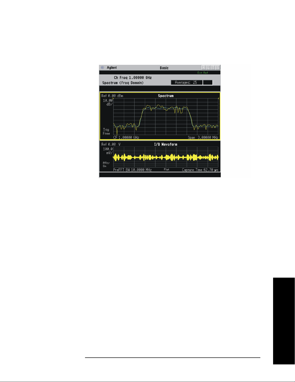
Making Measurements
Determining the RF Parameters of Your Signal
Figure 2-4 Spectrum Measurement - Spectrum and I/Q Waveform (Default
View)
Step 6. Press
measurement result display, including the following:
Spectrum - Provides a combination view of the Spectrum graph in
•
parameters of power versus frequency with semi-log graticules, and
the I/Q waveform graph in parameters of voltage and time. Changes
to the frequency span or power will sometimes affect data
acquisition. This is equivalent to changing the selected window with
the
Spectrum (Time Domain) I/Q Waveform - This graph is shown below the
Spectrum graph in the default dual-window display. I/Q Waveform
provides a view of the I/Q waveform in parameters of voltage versus
time in linear scale. Changes to sweep time or resolution bandwidth
can affect data acquisition.
View/Trace to display a menu allowing selection of another
Next Window key.
Making Measurements
Chapter 2 35
Page 36

Making Measurements
Determining the RF Parameters of Your Signal
Figure 2-5 Spectrum (Time Domain) Measurement - I/Q Waveform Result
Step 7. To make a measurement repeatedly, press
toggle the setting from
Single to Cont.
Meas Control, Measure to
Step 8. For PSA, if Option 122 or 140 is installed, you may use the wideband IF
hardware to view a wide bandwidth signal in the Spectrum view. The
I/Q Waveform view will be correctly demodulated to the I and Q
components over the entire display bandwidth.
•Press
MODE, and select Modulation Analysis to be able to use the
Wideband IF path.
•Press
•Press
MEASURE, and select the Spectrum measurement.
MEAS SETUP and toggle the IF Path key to select Wide. Adjust
the span to view up to 80 MHz for Option 122, or up to 40 MHz for
Option 140 around your selected center frequency.
The example shown below is a 54 carrier OFDM signal which has a
− 10 dB bandwidth greater than 16 MHz, with skirts to over twice that
bandwidth. Delta markers are shown measuring the peak bandwidth.
Making Measurements
36 Chapter 2
Page 37

Making Measurements
Determining the RF Parameters of Your Signal
Figure 2-6 Spectrum Measurement - Spectrum Zoom View with Opt. 122−
80 MHz Bandwidth Digitizer Hardware
Chapter 2 37
Making Measurements
Page 38

Making Measurements
Determining the RF Parameters of Your Signal
The example shown below is a 802.11 WLAN signal which has an
instantaneous bandwidth of over 36 MHz. Only the Average trace is
displayed.
When using the widest spans, the Resolution Bandwidth may be
limited by the maximum number of points available for a Spectrum
measurement. If your desired setting exceeds the available number of
points, the maximum number available will be used, and an error
message will be displayed.
Figure 2-7 Spectrum Measurement - Spectrum Zoom View with Opt. 122−
80 MHz Bandwidth Digitizer Hardware
Making Measurements
38 Chapter 2
Page 39

Making Measurements
Determining the RF Parameters of Your Signal
The example shown below is a Spectrum View of the center 20 MHz of a
Noise Power Ratio measurement. If you extend the Span to the full 80
MHz bandwidth, individual carriers displayed may merge, as they can
be limited by screen resolution and resolution bandwidth. Only the
Average data trace is displayed in the example below.
Figure 2-8 Spectrum Measurement - Spectrum View with Opt. 122− 80 MHz
Bandwidth Digitizer Hardware
Chapter 2 39
Making Measurements
Page 40
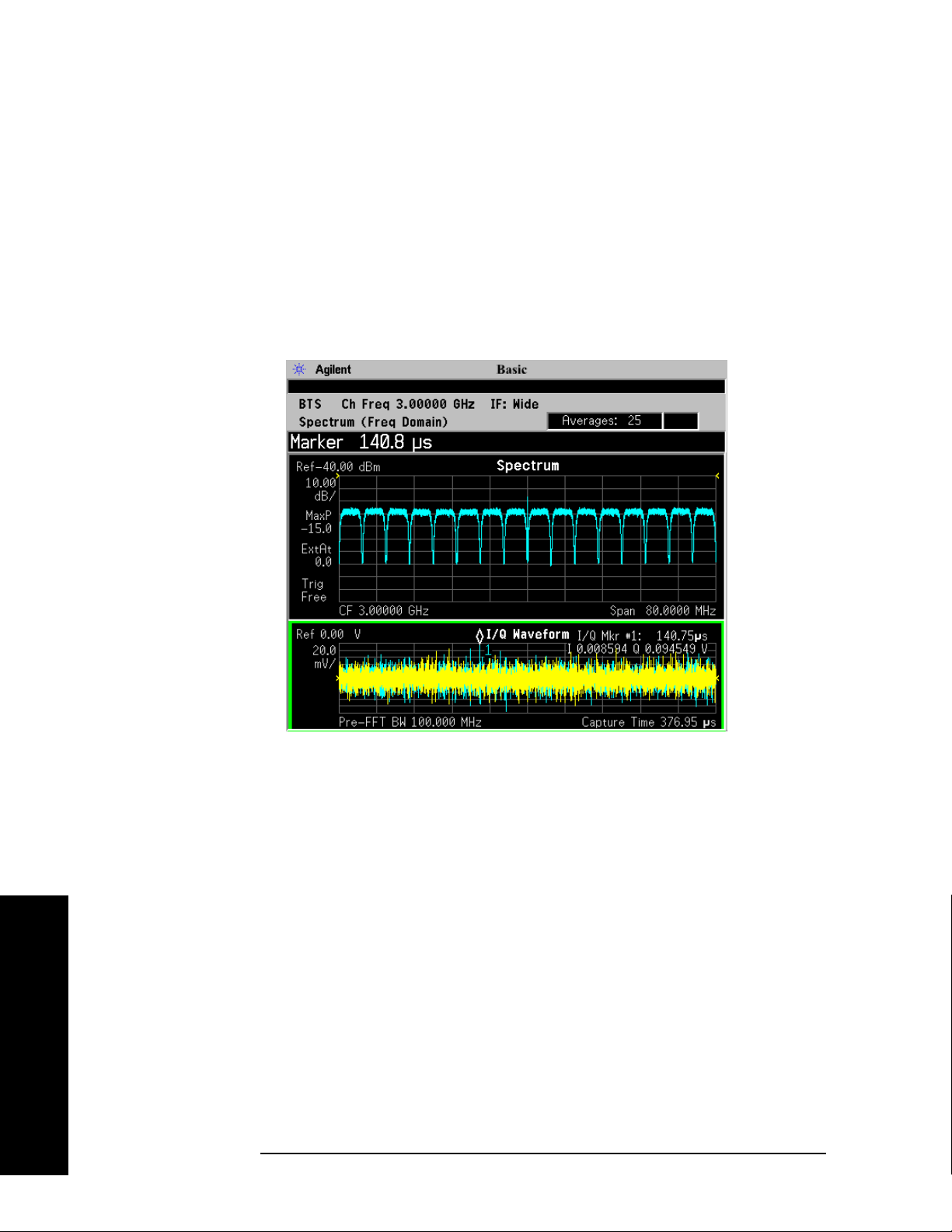
Making Measurements
Determining the RF Parameters of Your Signal
The wideband signal example shown below is 16 W-CDMA carriers,
each occupying 5 MHz of bandwidth. The full 80 MHz of available
demodulation bandwidth for the Spectrum measurement is used. Only
the Average trace is displayed. Note the demodulated composite I/Q
waveform for the entire 80 MHz BW signal in the
I/Q Waveform window
below. A peak search marker has been applied to the composite
waveform.
Figure 2-9 Spectrum Measurement - Spectrum Zoom View with Opt. 122−
80 MHz Bandwidth Digitizer Hardware
Making Measurements
Step 9. Press
measurement parameters from the default condition.
For more details about using PSA Wide Bandwidth BW Digitizing
Hardware Options 122 and 140, including detailed functional
descriptions and SCPI commands and concepts, see the PSA Basic
Mode Guide.
40 Chapter 2
Meas Setup, More to check the keys available to change the
Page 41

Determining the RF Parameters of Your Signal
Using the Waveform Measurement to Set Up Triggering (for burst signals)
You can use the waveform measurement to view your signal in the time
domain and to help select the appropriate trigger to acquire your signal.
Step 1. Activate the waveform measurement view:
Making Measurements
Press
MEASURE, Waveform (Time Domain).
Step 2. Adjust the scale of the x-axis to view the complete signal waveform:
Press
the scale/div, then press a units key, like
SPAN X Scale, Scale/Div, then use the front-panel keypad to input
µs, to complete the entry.
Step 3. Select a trigger source (free run is the default setting):
Press
Meas Setup, Trig Source, then select one of the available trigger
sources.
Triggering is unnecessary for most signals. For TDMA and other burst
signals, PSA Option 241 will readily acquire a “framed” signal.
NOTE In the waveform measurement the Burst/Sync Search menu is not
available.
measure mode.
Burst/Sync Search is available in the Modulation Analysis
Frame Timer (located under the Trig S e t up menu) must be
used to trigger on framed signals in the Waveform measurement.
Step 4. Set up the trigger conditions:
Press
Trig or Mode Setup, Trigg e r Setup , then choose a trigger mode.
In the trigger mode set the delay, peak level and positive or negative
edge slope trigger. You can also set up trigger holdoff, auto trigger
timing and frame timer settings.
Chapter 2 41
Making Measurements
Page 42

Making Measurements
Determining the RF Parameters of Your Signal
NOTE You can modify the trigger setup settings in an editable table view
under the
Mode Setup, Trigger Setup... key. You may select any
parameter to change the settings by pressing the Left/Right Arrow
keys. The current selection is highlighted in yellow or blue. You may
use the Up/Down Arrow keys, front-panel knob or the front-panel
keypad to input changes to the selected field.
Waveform (Time Domain) Measurements
This section explains how to make Waveform (Time Domain)
measurements on a cellular base station. Measurement of I and Q
modulated waveforms in the time domain disclose the voltages which
comprise the complex modulated waveform of a digital signal.
If installed, you may use PSA Option 122, the 80 MHz Bandwidth
Digitizer hardware, or PSA Option 140, the 40 MHz Bandwidth
Digitizer hardware to perform Waveform measurements of wideband
signals using Basic Mode.
Configuring the Measurement System
The base station (BTS) under test has to be set to transmit the RF
power remotely through the system controller. This transmitting signal
is connected to the instruments RF input port. Connect the equipment
as shown. An interfering or adjacent signal may supplied as shown.
From the base transmission station simulator (signal generator) and
the system controller, set up a call using loopback mode for the MS to
transmit the RF signal.
Figure 2-10 Waveform Measurement System
Making Measurements
42 Chapter 2
Page 43

Making Measurements
Determining the RF Parameters of Your Signal
1. Using the appropriate cables, adapters, and circulator, connect the
output signal of the BTS to the RF input of the instrument.
2. Connect the base transmission station simulator or signal generator
to the BTS through a circulator to initiate a link constructed with
sync and pilot channels, if required.
3. Connect a BNC cable between the 10 MHz OUT port of the signal
generator and the EXT REF IN port of the instrument.
4. Connect the system controller to the BTS through the serial bus
cable to control the BTS operation.
5. Connect an external trigger, if needed. Press
Mode Setup, Tr ig g e r to
access a menu to set up inputs and levels for all triggers. You must
then select the appropriate trigger under the
Meas Setup, Trigger
menu to direct the measurement to use your trigger settings.
Setting the BTS From the mobile simulator (signal generator) and the system controller,
set up a call using loopback mode for the BTS to transmit the RF signal.
Measurement Procedure
Step 1. Press
Step 2. Press
Preset to preset the instrument.
MODE, Digital Modulation key to enable the Digital Modulation
Mode measurements.
Step 3. To set the measurement center frequency, press
FREQUENCY Channel
and enter a numerical frequency using the front-panel keypad.
Complete the entry by selecting a units key, like
Step 4. Press
Press
Step 5. Press
The default display shows both
SPAN and enter a numerical span using the front-panel keypad.
MHz to set the measurement span in MHz.
MEASURE to initiate the Waveform measurement.
Current (yellow trace) and Average (blue
MHz.
trace) data. To make viewing the display easier, you can view either the
Current or Average trace separately.
•Press
display.
Step 6. Press
shown at a convenient time scale for viewing.
If installed, you may use the 80 MHz Bandwidth hardware to view a
wideband signal in the RF Envelope view.
Press
up to 80 MHz around your selected center frequency.
The following figure shows an example of an
Waveform (Time Domain) measurement. The measured values for the
Chapter 2 43
Trace/View, Trace Display, and select the trace(s) desired for
SPAN X Scale, and the up or down arrow key until the waveform is
Making Measurements
SPAN and select the Wideband RF Path. Adjust the span to view
RF Envelope result for a
Page 44

Making Measurements
Determining the RF Parameters of Your Signal
mean power and peak-to-mean power are shown in the text window.
Figure 2-11 Waveform Measurement - RF Envelope (Default View)
Step 7. Press
Trace/View to display the menu allowing selection of the other
Waveform views, including the following:
I/Q Waveform - Provides a view of the I and Q waveforms together on
•
the same graph in parameters of voltage versus time in linear scale.
Changes to the sweep time or resolution bandwidth can affect data
acquisition.
Step 8. If PSA Option 140 or 122 is installed, you may use the 40 or 80 MHz
Bandwidth hardware to view a wideband signal in the Waveform view.
Even if you are not interested in a wideband signal, using the
Wideband IF path provides powerful measurement flexibility, including
to the ability to accurately set practically any sample rate and thereby
resample waveforms. Resampling, or oversampling, at the correct rate
allows you to effectively obtain an integer number of samples per
symbol. Make sure that the sample time is aligned with the decision
points of the symbols to make analysis of measurement data much
easier.
The following example of performing a Wideband IF Waveform
measurement of a GSM burst will show the technique to accurately
align and resample a signal:
•Press
Mode, and select Modulation Analysis to be able to use the 80
MHz IF path.
Making Measurements
•Press
44 Chapter 2
MEASURE, and select the Waveform measurement.
Page 45

Determining the RF Parameters of Your Signal
•Press Trace/View and select the RF Envelope view.
Making Measurements
•Press
SPAN and toggle the IF Path key to select Wide. Adjust the span
to view up to 80 MHz around your selected center frequency. Note
the example below has 1 million data points.
Figure 2-12 Waveform Measurement - RF Envelope View with Opt. 122− 80
MHz Bandwidth Digitizer Hardware
• Make sure that your samples are synchronized to the decision points
of the signal of interest. In this case we will use the internal Frame
Timer to trigger our measurement. A GSM frame is 4.615383 ms
long.
Press
Mode Setup, Tri g g er, select Frame Timer, then select Period.
Enter 4.615383 ms. This only sets the frame timer period. You
must direct the measurement to use the Frame Timer in the next
step:
Press
Meas Setup, Trigge r S ource and select Frame.
For other measurements, an external trigger may be applied to an
External Trigger Input, on either the front or the real panel. You
must specify that trigger selection in this menu.
• In this example, we want to capture an entire GSM burst of 144
symbols (plus guard). A GSM burst is approximately 4.6 ms, so we
will set our
Meas Time to 5 ms:
Making Measurements
Chapter 2 45
Page 46

Making Measurements
Determining the RF Parameters of Your Signal
Press Meas Setup, Meas Time and enter 5 ms.
• In this resampling example, we want to take exactly 10 samples per
GSM symbol. The GSM symbol rate is 270.833 kHz, so we want a
sample rate of 2.70833 MHz. Option 122 Wideband IF hardware lets
us set the desired sample rate, as follows: sample rate = 5/4 IF
Bandwidth. That means we need set an IF BW of 2.16667 MHz.
Press
Meas Setup, IF BW and enter 2.16667 MHz.
You can also access the sample rate key directly:
Press
Rate
Meas Setup, Wideband Setup, Sample Rate. Enter the Sample
frequency. The Sample Rate and IF BW settings are coupled. The
5/4 ratio will be preserved regardless of which setting is used.
Figure 2-13 Waveform Measurement - RF Envelope View with Opt. 122−
80 MHz Bandwidth Digitizer Hardware
Making Measurements
For more details about making wideband measurements, see “PSA
Option 122 Wideband Digitizer” in the Option 122 section in the “PSA
Basic Mode Guide.”
Step 9. Press
waveforms are shown at a convenient voltage scale for viewing.
Step 10. Press
waveforms are shown at a convenient time scale for viewing.
46 Chapter 2
AMPLITUDE Y Scale and the up arrow or down arrow key until the
SPAN X Scale and the up arrow or down arrow key until the
Page 47

Making Measurements
Determining the RF Parameters of Your Signal
Step 11. Press Marker, Tra ce, I/Q Waveform to activate a marker. Rotate the RPG
knob until the marker is shown at a desired time in the waveform for
viewing the trace values at the time position of the marker.
Step 12. To make a measurement repeatedly, press
toggle to
Step 13. Press
Cont.
Meas Setup, More to check the keys available to change the
Meas Control, Measure and
measurement parameters from the default condition.
Using the Waveform Measurement to Set Up Triggering (for
burst signals)
You can use the Waveform measurement to view your signal in the time
domain and to help select the appropriate trigger to acquire your signal.
Step 1. Press
MEASURE, Waveform (Time Domain) to activate the Waveform
measurement view.
Step 2. Press
SPAN X Scale, Scale/Div to adjust the scale of the x-axis to view the
complete signal waveform. Use the front-panel keypad to input the
scale/div, then press a units key, like µs, to complete the entry.
Step 3. Press
Meas Setup, Trig Source, then select one of the available trigger
sources (free run is the default setting).
NOTE In the Waveform measurement, the Burst/Sync Search menu is not
available.
measurement mode.
must be used to trigger on framed signals in the
Burst/Sync Search is available in the Modulation Analysis
Frame Timer (located under the Trig Setup menu)
Waveform
measurement.
Step 4. Press
In the trigger mode, set the delay, peak level, and positive or negative
edge slope trigger. You can also set up trigger holdoff, auto trigger
timing, and frame timer settings.
For more details about using PSA Option 122, 80 MHz BW Digitizing
Hardware, and PSA Option 140, 40 MHz Digitizing Hardware,
including detailed function descriptions, SCPI commands, and
concepts, see the PSA Basic Mode Guide.
Chapter 2 47
Trig, then choose a trigger mode to set up the trigger conditions.
Making Measurements
Page 48

Making Measurements
Modulation Analysis Measurements in 8 Steps
Modulation Analysis Measurements in 8 Steps
NOTE PSA Option 241 can analyze digital modulation for a single code
channel only. If multiple code channels are transmitted,
synchronization will fail, and incorrect EVM results will be obtained.
For modulation quality measurements of multiple code channels,
Modulation Accuracy and Code Domain measurements must be
performed by a full-featured standard-based personality, like PSA
Option BAF for W-CDMA.
Step 1. Select the modulation analysis personality from the mode menu:
Press
MODE, Digital Modulation.
Step 2. Select the radio standard and device of your signal (if known):
Press
Press
Selecting a radio standard will preset the
Mode Setup, Radio, Radio Standard, then select a radio format.
Device, then select BTS or MS.
Meas Setup modulation
parameters to demodulate a standard radio signal.
Step 3. Activate the modulation analysis measurement:
Press
MEASURE, Modulation Analysis.
When you select Modulation Analysis, the PSA demodulates the radio
standard, selected in Step 2, based off of the preset modulation
parameters. If your signal has modulation properties that differ from
the preset radio standards, follow steps 4 through 7 to modify the
modulation parameters.
Step 4. Select a modulation format:
Press
Meas Setup, Demod, Modulation Format, then select the modulation
format of your signal from the available selections.
TIP If you do not know the modulation format of your signal, identifying an
unknown signal format is a significant challenge requiring specialized
expertise. For more information on this subject see, “Modulation
Formats and Applications” on page 203.
Making Measurements
Step 5. Set the symbol rate of your signal:
Press
to input a numerical rate, then press a units key, like
Meas Setup, Demod, Symbol Rate, then use the front-panel keypad
kHz, to complete
the entry.
Step 6. Select the measurement filter type, the reference filter type and the
filter roll-off (alpha) value:
48 Chapter 2
Page 49

Making Measurements
Modulation Analysis Measurements in 8 Steps
Press Meas Setup, Demod, Meas Filter, then select a filter type.
Press
Press
Meas Setup, Demod, Ref Filter, then select a filter type.
Meas Setup, Demod, Alpha/BT, then enter a numeric value.
When selecting the filter types, remember: the “measured” filter should
simulate the intended receiver, while the “reference” filter should
match the product of the transmitter and receiver filters.
TIP If the alpha/BT is unknown, you can make a starting estimate based on
the signal bandwidths as follows: (−60 dB BW / −3 dB BW) – 1.
EVM peaks between symbols mean an incorrect alpha, but won’t
usually affect the EVM% readout (except in GSM). In the worst case,
start with an alpha of 0.3 and manually adjust up or down for lowest
intersymbol peaks.
Step 7. Select the measurement interval and the number of data points per
symbol for the measurement:
Press
to input an interval in symbols, and press
Press
Meas Setup, Demod, Meas Interval, then use the front-panel keypad
Enter to complete the entry.
Display, Pts/Symbol, then select 1, 2, 4, 5, or 10 points per symbol.
More points/symbol reveal more detail of the intersymbol waveforms
(for viewing eye diagrams, error peaks, etc.). The drawback of
demodulating using more points/symbol is a slower measurement.
TIP Result length is important for bursted signals, as you do not want to
include data symbols taken before or after the burst (that is, you do not
want to demodulate noise). See Concepts chapter for “PSA Digital
Demodulator” on page 281.
Step 8. Turn on Burst/Sync search for burst signals:
Press
Other burst search settings include
Length
TIP Maximum search length can be many times longer than a measurement
Meas Setup, Burst Sync/Search, Sync, then select a sync method.
Burst Search Threshold, Search
, Sync Pattern, Sync Word Length and Sync Offset.
length; set the search length to the burst “off” time plus twice the burst
“on” time to insure that a complete burst will always be captured.
Making Measurements
NOTE The settings described in steps 5 through 8 are also available in a single
location. Press
Meas Setup, Meas Setup... to see all the measurement
settings.
Chapter 2 49
Page 50

Making Measurements
Modulation Analysis Measurement Final Checks
Modulation Analysis Measurement Final
Checks
• The EVM% result should be fairly consistent from measurement to
measurement. Result peaks may indicate faulty triggering or
incorrect synchronization.
• EVM vs. symbol trace should be noise-like, but fairly uniform (short
peaks are OK). Abrupt changes within the EVM trace signify
problems, as do sloping or V-shaped distributions.
• Overall shape of eye and constellation diagrams are regular and
stable (even if individual symbols are very noisy, the characteristic
shape should be evident). Eye opening should line up precisely with
the display center line—if not, tweak “clock adjust” for best
centering (lowest EVM). See “Setting Advanced Measurement Setup
Properties” on page 59 for more information on setting clock adjust.
• If measurement results are variable, and you suspect low
signal-to-noise ratio is reducing your measurement accuracy, turn on
the analyzer internal preamplifier:
Press
Input/Output, More (1 of 2), Int Preamp (On).
• You may also be able to optimize the dynamic range of the
measurement by setting the RF input range as low as possible
without overload:
Press
Meas Setup, More, Advanced, ADC Range, Manual then select the
highest ADC gain value that may used without tripping the Input
Overload annunciator (at the lower edge of the spectrum display
screen).
Check: Increase ADC gain by 1 step; overload indicators should turn
on. Finer adjustments can be made by setting the internal RF
attenuation: you want to find the lowest ADC gain value that just
trips the Input Overload annunciator. Use one 2 dB attenuator
step lower than the attenuator setting that set the analyzer in
overload.
Press
Input/Output, Input Atten and select the lowest attenuation
value that can be used without tripping the Input Overload
annunciator.
Making Measurements
50 Chapter 2
Page 51

Making Measurements
Modulation Analysis Measurement Final Checks
• If these methods do not improve the “noisy” characteristics of your
measurement, you may need to supply more signal gain ahead of the
RF input to the analyzer. Make sure you use the analyzer’s ability to
correct for external gain and attenuation:
Press
Input/Output, Ext RF Atten and select either BTS or MS. You may
enter a positive number to correct for external attenuation or input a
negative number to correct the power measurements for external
gain.
NOTE When tuned above 3GHz, the PSA employs a YIG-tuned preselector
filter. This filter is required for full image protection, but it may be
bypassed if Option 123 Unpreselected High Band hardware is installed.
This option is especially useful when measuring band-limited signals in
the absence of any other signals. If the Microwave Preselector is
bypassed (OFF), then the IF frequency response at a given center
frequency is repeatable. See “Microwave Preselector” on page 127.
Chapter 2 51
Making Measurements
Page 52

Making Measurements
Modifying Measurement Setup Parameters
Modifying Measurement Setup Parameters
Using the Measurement Setup Form
The measurement setup form contains demodulation parameters,
averaging, triggering, burst/sync search parameters and equalization
parameters. It is useful for a quick overview of all the key measurement
settings without having to access each menu map individually to check
or modify settings.
This procedure demonstrates how to navigate and modify settings in
the measurement setup form. This procedure assumes you are already
in the
under the
Step 1. Access the measurement setup form:
Digital Modulation mode and you have selected Modulation Analysis
MEASURE menu.
Press
Meas Setup, Meas Setup...
Step 2. Navigate through the measurement setup settings:
Press
→ (right tab arrow), or ← (left tab arrow).
To modify the current settings, navigate to the parameter you want to
modify with the left or right arrow keys. If the input box is highlighted
in blue, you can use the soft key menu on the right of the display to
select your setting. If the input box is highlighted in yellow, use the
numeric keypad to enter a value and then select a unit key from the soft
key menu.
Figure 2-14 Measurement Setup Form with Preset Values (Radio=W-CDMA)
r
Making Measurements
52 Chapter 2
Page 53

If you are using a preset radio standard, the measurement settings are
preset for your measurement. Modify the settings to match your
modulation parameters or testing requirements.
Setting Demodulation Parameters
To demodulate customized digital formats, the demodulation
parameters can be modified. Choose from a wide range of basic digital
formats, measurement and reference filters, filter alpha/BT values and
symbol rates. By modifying demodulation parameters to improve EVM,
you can estimate what needs to be changed in your device under test to
meet your test specifications.
The following procedure demonstrates how to modify demodulation
parameters. This procedure assumes you are already in the
Modulation
MEASURE menu.
Step 1. Access the demodulation menu:
mode and you have selected Modulation Analysis under the
Making Measurements
Modifying Measurement Setup Parameters
Digital
Press
Meas Setup, Demod.
Step 2. Select a modulation format:
Press
Modulation Format, then select a format.
Modulation formats include BPSK, QPSK, 8PSK, DQPSK, D8PSK,
Pi/4 DQPSK, Offset QPSK, 16QAM, 32QAM, 64QAM, 128QAM,
256QAM, EDGE, 2FSK, 4FSK, 8FSK, MSK type1 and type2, DVB
QAM 16, 32, 64, 128, and 256.
Step 3. Select a measurement filter type:
Press
Meas Filter, then select a filter type.
Filter types include root nyquist, nyquist, gaussian, EDGE measured
filter (EMF), CDMA (IS-95 Base EQ), rectangle, and no filter.
Step 4. Select a reference filter type:
Press
Ref Filter, then select a filter type.
Filter types include root nyquist, nyquist, gaussian, EDGE and CDMA
(IS-95 Base), rectangle, and half sine.
When selecting the filter types, remember: the “measured” filter should
simulate the intended receiver, while the “reference” filter should
match the product of the transmitter and receiver filters.
Making Measurements
Chapter 2 53
Page 54

Making Measurements
Modifying Measurement Setup Parameters
Step 5. Enter a filter alpha/BT value:
Press
Alpha/BT, enter a numeric value, then press Enter.
Step 6. Enter a symbol rate:
Press
Symbol Rate, enter a numeric value, then select a unit.
Setting up a Trigger Source
For burst signals and TDMA (time division multiple access) signals, it
is necessary to use a trigger for RF and modulation analysis of the
signal.
For more detailed information on trigger types see “Measurement
Domains” on page 279.
This procedure reviews the available trigger source types. This
procedure assumes you are already in the
you have selected
Step 1. Access the trigger source menu:
Press
Meas Setup, Trigge r S ource.
Step 2. Select a trigger source from the list:
Free Run (Immediate) - Sets the trigger to start a new
•
sweep/measurement as soon as the last one has ended (continuous
sweep mode) or immediately (single sweep mode). Free run trigger is
completely asynchronous to the RF or IF signal.
Modulation Analysis under the MEASURE menu.
Digital Modulation mode and
Making Measurements
Video (IF Envlp) - Activates the trigger condition that allows the next
•
sweep to start if the detected RF envelope voltage crosses a level set
by the video trigger level.
RF Burst (Wideband) - An internal wideband RF burst trigger that
•
has an automatic level control for burst signals. It triggers on a level
that is relative to the peak of the signal passed by the RF.
Ext Front - Sets the trigger to start a new sweep/measurement
•
whenever the external voltage (connected to EXT TRIGGER INPUT
on the front panel) passes through approximately 1.5 volts.
Ext Rear - Sets the trigger to start a new sweep/measurement
•
whenever the external voltage (connected to TRIGGER IN on the
rear panel) passes through approximately 1.5 volts.
Frame - Sets the trigger to use the internal frame clock to generate a
•
trigger signal. The clock parameters are controlled in the Trig Setup
menu (under the Mode Setup key).
54 Chapter 2
Page 55

Making Measurements
Modifying Measurement Setup Parameters
Setting Burst/Sync Properties
Synchronization words (or patterns) are often used to resolve carrier
phase ambiguity on non-differential modulation formats. It is
important to realize that synchronization words are optional and are
not necessary to achieve carrier locking.
Sync search lets you use a synchronization pattern to isolate a segment
of your signal for display and analysis. The analyzer searches through
demodulated data to find your synchronization pattern and then uses
the
Sync Word Length to determine how many symbols to search as the
syncword.
Triggering is used to determine when the analyzer starts searching
syncword or burst in data and
analyzer stops searching.
Searching more detailed information on synchronization see “PSA
Digital Demodulator” on page 281.
This procedure demonstrates how to set burst/sync properties. This
procedure assumes you are already in the
you have selected
Modulation Analysis under the MEASURE menu.
Search Length determines when the
Digital Modulation mode and
Step 1. Access the synchronization menu:
Press
Meas Setup, Burst/Sync Search.
Step 2. Select the synchronization type:
Press
Available synchronization types include
Sync Word Burst and you have the option of selecting no sync type
(
Sync, then chose from one of the available sync types.
RF Ampl, Sync Word Cont,
None).
Step 3. Set the burst search threshold level for RF amplitude and sync word
burst synchronization types:
Press
Once the trigger requirements have been met and
Sync Word Burst is selected as a sync type, the burst must meet the
Burst Search Threshold, enter a numeric value, then press dB.
RF Ampl or
threshold level before the sync search starts. If the threshold level is
met, the analyzer will demodulate the burst for the time period set in
Search Length.
Step 4. Set the length of time you want to search the burst or the
synchronization pattern:
Making Measurements
Press
Search Length, enter a numeric value, then select a unit, like ms.
Your trigger signal determines when the analyzer begins accumulating
data for the search length. The analyzer begins to demodulate your
signal when it receives a valid trigger, and capture data for the duration
Chapter 2 55
Page 56

Making Measurements
Modifying Measurement Setup Parameters
of Search Length.
Step 5. Set the synchronization bit pattern in hexadecimal values:
Press
press
Sync Pattern, enter a bit pattern as hexadecimal values, then
Done
The synchronization pattern is used when Sync Word Cont or
Sync Word Burst is enabled as a sync search type. Sync Pattern is not
used when
RF Ampl sync search type is enabled.
Step 6. Set the length of the synchronization word length:
Press
Sync Word Length determines how many symbols are used as SyncWord.
Sync Word Length, enter a numeric value, then press Enter.
See “Sync Word Length” on page 161 for word length settings. The
Synchronization word length is used when
Sync Word Burst is enabled as a sync search type.
Sync Word Cont or
Step 7. Set the synchronization offset:
Press
Sync Offset, enter a numeric value, then press Enter.
Synchronization offset can be set from −1000 to 1000 symbols as
described in “Sync Offset” on page 161. Synchronization offset
determines the relative position of the measured data from the
beginning of the SyncWord; with respect to the start of the sync pattern.
Synchronization offset is used when
Sync Word Cont or Sync Word Burst
is enabled as a sync search type.
Making Measurements
Using Adaptive Equalization
Equalization removes linear errors from modulated signals by
dynamically creating and applying a FIR (feed-forward) compensating
filter. Using equalization allows measurement of impaired channels
and can be used to isolate linear from non-linear error mechanisms. For
more concept information on equalization see “Modulation quality
measurements” on page 286.
This procedure demonstrates how to setup the equalizer. This
procedure assumes you are already in the
you have selected
Step 1. Access the equalization menu:
Press
Meas Setup, More, Equalization.
Step 2. Set the equalization filter length:
Press
EQ Filter Length, enter a numeric value, then press Enter.
Available filter length values include 3, 5, 7 and 99 symbols.
When selecting a filter length, the best filter length is the smallest that
Modulation Analysis under the MEASURE menu.
Digital Modulation mode and
56 Chapter 2
Page 57

meets your measurement requirements. For example, measurements at
the transmitter may only need a few symbols in length. Measurements
in multi-path environments require longer filter lengths.
Step 3. Set the equalization convergence:
Making Measurements
Modifying Measurement Setup Parameters
Press
EQ Convergence, enter a numeric value, then press Enter.
You can set convergence values from 0.001 to 100.
Convergence determines how quickly the equalization filter coefficients
converge to the estimated values for each measurement. Larger values
converge faster. Values set too large can cause the adaption algorithm
to become unstable, limiting the minimum EVM or SNR.
TIP At the start of your measurement set the convergence high, to quickly
shape the filter. Then decrease the convergence to fine-tune the filter to
the optimum shape to get the best EVM results.
Step 4. Turn the equalization filter on:
Press
EQ Filter (On).
When equalization is first enabled, the equalization filter has a unit
impulse response. The length of the filter determines the position of the
unit impulse response in the filter. The impulse is located in the center
of the filter for short filter lengths. As the filter length increases, the
impulse moves, proportionally, towards the start of the filter to handle
channels with large delay-spread.
The equalization filter has a unit response when you:
• First run the equalizer.
• Reset the equalizer filter
• Change points/symbol
• Change the measured or reference filter
• Change the symbol rate
• Change the clock delay adjustment
• Change the equalizer filter length
• Change the modulation format
•Preset the mode
Aside from the above conditions, the equalizer uses the last computed
filter coefficients when you enable equalization. For example, if you
used equalization in a previous measurement, the coefficients from the
previous measurement are used, unless you reset the equalization filter
(or change one of the settings as mentioned in the above list). It is good
Making Measurements
Chapter 2 57
Page 58

Making Measurements
Modifying Measurement Setup Parameters
practice to reset the equalization filter to initialize the filter coefficients
before starting the measurement.
Step 5. Reset the equalization filter:
Press
Reset EQ Filter. Once you reach the desired EVM results after
resetting the equalization filter, hold the filter coefficient values.
Step 6. Hold the filter coefficient values:
Press
EQ Hold (On). When EQ Hold is on, the analyzer does not update
the filter coefficients. Instead, the analyzer uses the last updated
coefficients before selecting hold.
When
EQ Hold is off, the analyzer uses the results of the current
measurement to update the filter coefficients for the next
measurement. The equalization algorithm chooses coefficients that
produce a modulation quality result that is less impacted by the
presence of linear distortion.
Step 7. You can view the equalizer graphically:
Press
Trace/View, Equalizer (Quad View). The Ch Frequency Response
trace shows the frequency response channel for which the equalizer is
correcting. Ch Frequency Response is computed as the inverse of the
equalization filter's frequency response. The data is complex and is
normally displayed in units of magnitude and phase.
The Eq Impulse Response trace shows the impulse response of the
equalization filter. The example shown in Figure 2-15 is an EDGE
signal.
Making Measurements
58 Chapter 2
Page 59
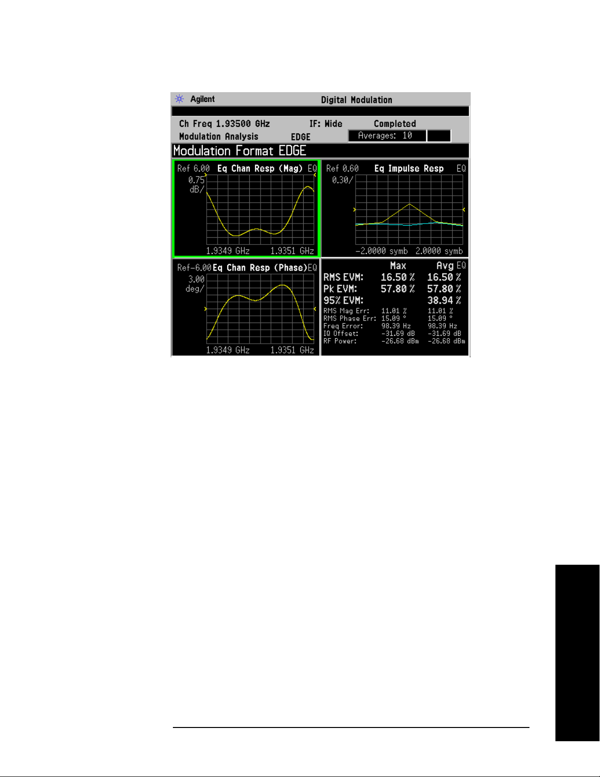
Modifying Measurement Setup Parameters
Figure 2-15 Equalizer View - EDGE Signal Example
Making Measurements
Setting Advanced Measurement Setup Properties
Advanced measurement features give you additional flexibility in
setting measurement limits, adjusting the clock, setting the IF
bandwidth and setting the analyzer ADC range.
This procedure demonstrates how to set advanced measurement
properties. You can jump from step 1 to any other step in this procedure
if you need to access a certain advanced setting. This procedure
assumes you are already in the
selected
Modulation Analysis under the MEASURE menu.
Step 1. Access the advanced measurement menu:
Press
Meas Setup, More, Advanced.
Step 2. Modify the pass/fail limit for RMS EVM:
Press
Limits, RMS EVM, enter a numeric value, then press %.
When you enter a numeric value the limit turns on automatically. To
toggle the limit off and on press
Step 3. Modify the pass/fail limit for frequency error:
Press
terminator, like
Limits, Freq Error, enter a numeric value, then select a unit
kHz.
Digital Modulation mode and you have
RMS EVM.
Making Measurements
When you enter a numeric value the limit turns on automatically. To
Chapter 2 59
Page 60

Making Measurements
Modifying Measurement Setup Parameters
toggle the limit off and on press Freq Error.
Step 4. Mirror (invert) the frequency spectrum about the analyzer center
frequency for correct demodulation:
Press
By pressing
Spectrum (Invert).
Spectrum you can toggle the frequency spectrum between
normal and inverted. The default spectrum setting is Normal.
Often, when a signal is mixed down from a higher frequency, the
spectrum is flipped or mirrored about the center frequency as a result of
the mixing scheme used. A mirror spectrum occurs when the frequency
of the mixer’s LO is higher than the frequency of the signal being
measured.
Step 5. Modify clock adjust (in symbols) to determine when the demodulator
samples the I/Q trajectory:
Press
Clock Adjust, enter a numeric value, then press Enter.
Clock adjust can be set from −0.5 to +0.5 symbols. Zero (0) symbols is
the default value.
Some digital communications systems contain non-linearity’s that can
bias the digital demodulator’s estimation of the symbol clock position.
Use clock adjust to compensate for this offset and obtain a lower EVM.
You can see the effects of changing clock adjust by displaying a
constellation diagram or eye diagram. Increasing (or decreasing) clock
adjust:
Making Measurements
• Shifts the detection-decision points in the constellation diagram.
• Slides the eye diagram right or left (remember that in the eye
diagram, the symbol locations remain in a fixed location on the
display; therefore, changing the location of symbols has the effect of
horizontally shifting of the eye diagram).
60 Chapter 2
Page 61

Making Measurements
Modifying Measurement Setup Parameters
Step 6. Toggle the EVM reference calculation between mean and max:
Press
EVM Ref Calc.
The EVM reference calculation is available when demodulating one of
the QAM formats. When
EVM Ref Calc is set to mean, the mean
magnitude of all QAM decision points are used as the reference. When
it is set to max, the magnitude of the decision points with the largest
distance from the origin are used as a reference.
Step 7. Modify the IF bandwidth setting:
Press
like
IF Bandwidth (Man), enter a numeric value, then select a unit key,
MHz. For the optimum EVM accuracy, IF Bandwidth should
encompass all the significant power spectral density of the channel.
If installed, PSA Option 122, 80 MHz Bandwidth Digitizer hardware
may be used to capture up to 80 MHz of signal spectrum. Press
Setup
, More, IF Path, and toggle the setting to Wide to increase the
available IF bandwidth of the instrument. See “Wideband Setup” on
page 171 for more details of using the wideband IF path.
The default state is set to auto. If no radio standard is selected, the
default setting is 10 MHz. The maximum setting is 10 MHz and the
minimum setting is 1 kHz.
When the
IF Bandwidth is set to auto, the IF bandwidth is determined
based on the radio standard format and symbol rate
(IF Bandwidth = symbol rate x 4).
Meas
Step 8. Select an ADC ranging method:
Press
The
Peak
•
•
ADC Range, then select an ADC range type.
ADC Range default is set to Auto. You can select from Auto, Auto
, AutoPeakLock and Manual:
Auto - Select this to set the ADC range automatically.
Auto Peak - Select this to set the ADC range automatically to the
peak signal level. Auto peak is a compromise that works well for
both CW and burst signals.
AutoPeakLock - Select this to hold the ADC range to the peak signal
•
level.
Manual - Select from one of the following ADC range levels: 0 dB, +6
•
dB
, +12 dB, +18 dB or None. Select None to lock the range at the
present value. Manual range settings provides the best
measurement results for CW signals.
Making Measurements
Chapter 2 61
Page 62

Making Measurements
Measuring Digital Modulation Formats
Measuring Digital Modulation Formats
Modulation Analysis Measurement Views
To help pin-point modulation problems, the modulation analysis
personality provides I/Q polar graphs, EVM versus time graphs, eye
diagrams and numeric results tables. The following procedures show
you how to navigate through the results displays using a W-CDMA
signal (Bluetooth is used for the FSK displays).
• “Setting up the Modulation Analysis Personality” on page 63
• “Viewing the I/Q Polar Vector and Constellation Graphs” on page 64
• “Viewing the Numeric Measurement Results” on page 66
• “Viewing the I/Q Error (Quad-View) Results” on page 67
• “Viewing the Magnitude Error Versus Time Results” on page 68
• “Viewing the Phase Error Versus Time Results” on page 70
• “Viewing the EVM Versus Time Results” on page 73
• “Viewing the Eye Diagram Results” on page 75
• “Viewing the FSK Error (Quad-View) Results” on page 77
• “Viewing the FSK Error Versus Time Results” on page 79
• “Viewing the FSK Error Spectrum Results” on page 81
• “Viewing the FSK Measured Time Results” on page 83
Modulation Analysis Examples
The following examples analyze industry standard wireless
communication signals for each family of the basic digital modulation
formats.
• “PSK Modulation Analysis (cdma2000 QPSK Example)” on page 85
• “QAM Modulation Analysis (64QAM Example)” on page 87
• “EDGE Modulation Analysis” on page 89
• “FSK Modulation Analysis (Bluetooth 2FSK Example)” on page 91
• “MSK Modulation Analysis (GSM MSK type 1 Example)” on page 93
For a list of all available basic digital formats and pre-set radio
standard formats see “Digital Modulation Format Standards” on
page 203.
Making Measurements
62 Chapter 2
Page 63

Making Measurements
Measuring Digital Modulation Formats
Setting up the Modulation Analysis Personality
This procedure is the first step toward making any measurements with
the modulation analysis personality.
Configuring the Measurement System
Refer to “Configuring a BTS Measurement System” on page 29 to
connect the measurement equipment.
Agilent ESG Series Vector Signal Generator Settings
Radio Standard: W-CDMA (3GPP)
Link: Forward
Active channel: 1 DPCH (data channel)
Frequency: 1 GHz
Power (Signal Amplitude): -20 dBm
Modulation: QPSK
Filter: WCDMA, 0.22 alpha
Symbol rate: 3.84 Msps
Measurement Procedure
If you have a problem, and get an error message, see “Interpreting
Error Codes” on page 119.
Step 1. Preset the instrument and select the digital modulation personality:
Press
Press
Preset, Factory Preset (if available).
MODE, Digital Modulation.
Step 2. Select the W-CDMA pre-set radio standard and base station device:
Press
Press
Mode Setup, Radio, Radio Standard, WCDMA.
Device (BTS), to underline BTS.
Step 3. Set the center frequency to 1 GHz.
Press
FREQUENCY Channel, Center Freq, 1, GHz.
Step 4. Enable the modulation analysis mode to measure and display EVM and
other modulation metrics.
Press
MEASURE, Modulation Analysis.
The default view for the modulation analysis personality is the I/Q
Measured Polar Vector graph (see Figure 2-16).
Making Measurements
Chapter 2 63
Page 64
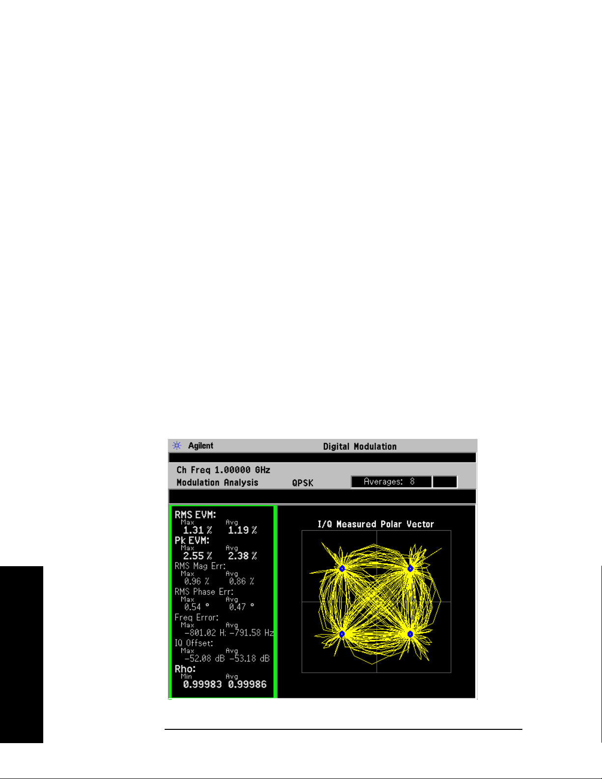
Making Measurements
Measuring Digital Modulation Formats
Viewing the I/Q Polar Vector and Constellation Graphs
This procedure demonstrates the different views of the I/Q measured
polar graphs. The I/Q polar graphs can show symbol point trajectories
(inter-symbol data) and constellation points at the same time or
individually. A common example of viewing the vector (inter-symbol)
data is to determine if the filter roll-off value (alpha) is set too steep or
shallow as shown by the length of the trajectory past the symbol point.
Measurement Procedure
If you have a problem, and get an error message, see “Interpreting
Error Codes” on page 119.
Step 1. Follow the procedure “Setting up the Modulation Analysis Personality”
on page 63 before continuing.
Step 2. View the I/Q measured polar graph with vector data and constellation
points (this is the default view):
Press
Trace/View, I/Q Measured Polar Graph.
The default view for the modulation analysis personality is the I/Q
Measured Polar Vector graph (see Figure 2-16). The measurement
values for EVM, magnitude error, phase error, frequency error, I/Q
offset and rho are shown in the summary window on the left side of the
display.
Figure 2-16 I/Q Measured Polar Vector Graph (Default View)
Making Measurements
64 Chapter 2
Page 65

Measuring Digital Modulation Formats
Step 3. View the I/Q measured polar graph with vector (inter-symbol data) or
constellation points only. Press
Vec tor da t a ( Figure 2-17). Press
Display, I/Q Polar Type, Vector to see
Display, I/Q Polar Type, Constellation to
see Constellation data (Figure 2-17).
Figure 2-17 I/Q Measured Polar Graph - Polar Vector View
Making Measurements
Figure 2-18 I/Q Measured Polar Graph (Left - Vector, Right - Constellation)
Making Measurements
Chapter 2 65
Page 66
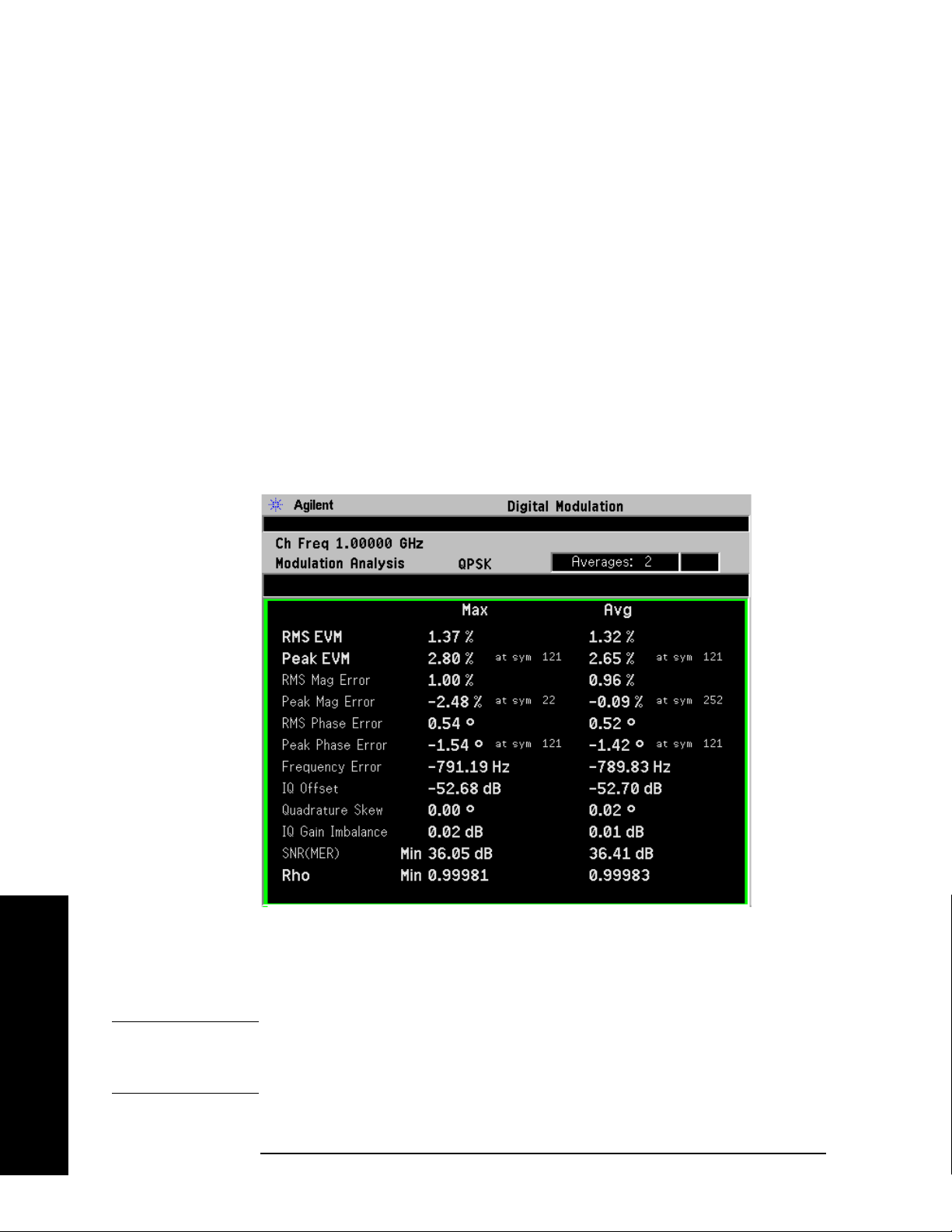
Making Measurements
Measuring Digital Modulation Formats
Viewing the Numeric Measurement Results
The numeric results provide you with the most important modulation
results to determine where the problem might lie. It’s a good starting
point to compare results side-by-side and decide which measurement
view to go to next.
Measurement Procedure
If you have a problem, and get an error message, see “Interpreting
Error Codes” on page 119.
Step 1. Follow the procedure “Setting up the Modulation Analysis Personality”
on page 63 before continuing
Step 2. Select the numeric results view:
Press
Trace/View, Numeric Results.
Figure 2-19 Numeric Results View (QPSK Example)
Making Measurements
The numeric results summary table shows modulation data including
maximum and average values for EVM, magnitude error, phase error,
frequency error, I/Q offset, quadrature skew, I/Q gain imbalance, SNR
and Rho.
NOTE The numeric result types differ between modulation formats. For
example, FSK results don’t provide phase results. See “FSK Modulation
Analysis (Bluetooth 2FSK Example)” on page 91 for more information.
66 Chapter 2
Page 67
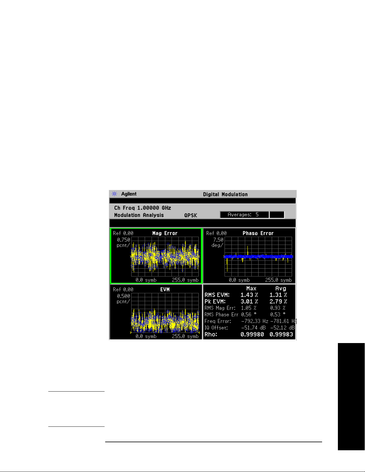
Making Measurements
Measuring Digital Modulation Formats
Viewing the I/Q Error (Quad-View) Results
This procedure demonstrates the different views of the I/Q error
quad-view. The I/Q error quad-view allows you to see the magnitude
error versus time, phase error versus time, EVM versus time and a
numeric summary table all on one screen to quickly determine any
impairments that may exist. You can zoom in on each of the 4 views for
more resolution to help pin-point any problems.
If you have a problem, and get an error message, see “Interpreting
Error Codes” on page 119.
Step 1. Follow the procedure “Setting up the Modulation Analysis Personality”
on page 63 before continuing.
Step 2. View the I/Q error quad-view:
Press
Trace/View, I/Q Error (Quad-View).
Figure 2-20 I/Q Error (Quad-View)
The I/Q error quad-view measurement result displays three graphs and
one numeric results summary table. The graphs consist of Mag Error
versus symbol, Phase Error versus symbol and EVM versus symbol. The
numerical results table shows key modulation metrics as maximum and
average values associated with the last demodulated capture period.
NOTE Using the Next Window key, you can scroll through the measurement
displays, where the current selection is highlighted with a green box
outline. The
Zoom key will zoom in on the currently selected display. To
go back to the quad-view display press Zoom again.
Chapter 2 67
Making Measurements
Page 68

Making Measurements
Measuring Digital Modulation Formats
Viewing the Magnitude Error Versus Time Results
This procedure shows you how to adjust x-axis and y-axis settings for
the magnitude error versus time graph. By zooming into a time capture
area of interest, modulation magnitude errors can be identified easier.
If you have a problem, and get an error message, see “Interpreting
Error Codes” on page 119.
Step 1. Follow the procedure “Setting up the Modulation Analysis Personality”
on page 63 before continuing.
Step 2. View the I/Q error quad-view (see Figure 2-20):
Press
Trace/View, I/Q Error (Quad-View).
Step 3. View the zoomed-in graph of magnitude error versus symbol. Use
markers to look at the magnitude error of individual symbol points.
Press
Press
NOTE Using the Next Window key, you can scroll through the measurement
Zoom.
Marker, Trace, Mag Error.
displays, where the current selection is highlighted with a green box
outline. The
Zoom key will zoom in on the currently selected display. To
go back to the quad-view display press Zoom again.
Figure 2-21 I/Q Error: Magnitude Error versus Symbol
Making Measurements
The Mag Error measurement display shows the magnitude error
versus symbol. Depending on the number of symbols captured in the
Meas Interval key, by measurement default parameters, the x-axis
displays symbols 0 through 1 minus the
68 Chapter 2
Meas Interval
Page 69
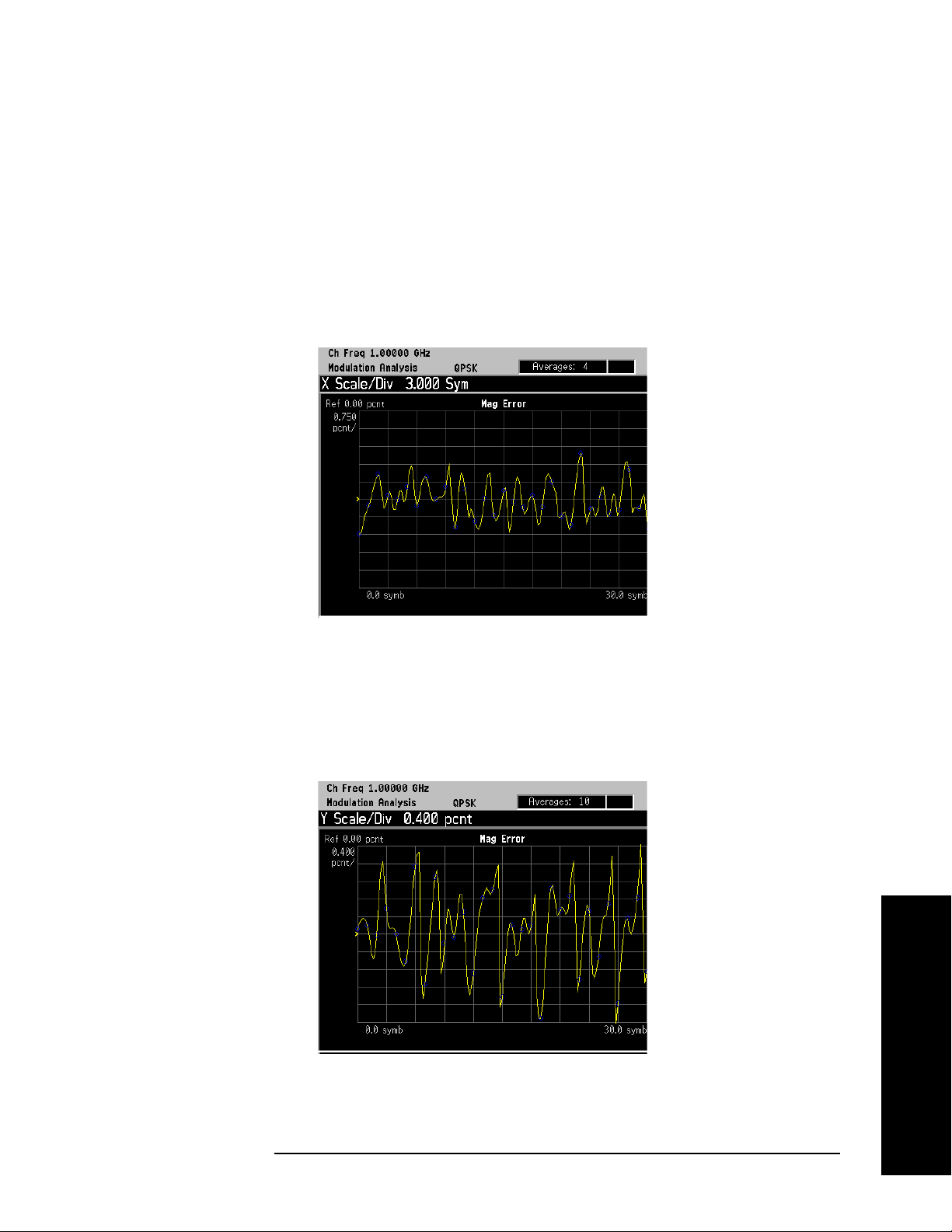
Making Measurements
Measuring Digital Modulation Formats
Step 4. Change the x-axis settings to zoom in on smaller portion of the
measurement capture interval:
Press
SPAN X Scale, Scale/Div, 3, Symbols.
To place the symbol points on the vertical graticules, use integer symbol
values for
reduce the measurement interval with the
to view another portion of the time capture interval, adjust the
Val ue
Scale/Div. An alternate method to view less symbols is to
Meas Interval key. If you want
Ref
.
Figure 2-22 I/Q Error: Magnitude Error versus Symbol (X-Axis Settings)
The Mag Error measurement displayed in Figure 2-22 shows an x-axis
Scale/Div of 3 with a measurement capture interval of 256 symbols.
Step 5. Decrease the y-axis settings to increase the resolution of the magnitude
error results. Use the same x-axis settings from the previous step.
Press
AMPLITUDE Y Scale, Scale/Div, 0.4, %.
Figure 2-23 I/Q Error: Magnitude Error versus Symbol (Y-Axis Settings)
The Mag Error measurement displayed in Figure 2-23 shows a y-axis
Scale/Div
of 0.4 percent and a reference level of 0 percent.
Making Measurements
Chapter 2 69
Page 70
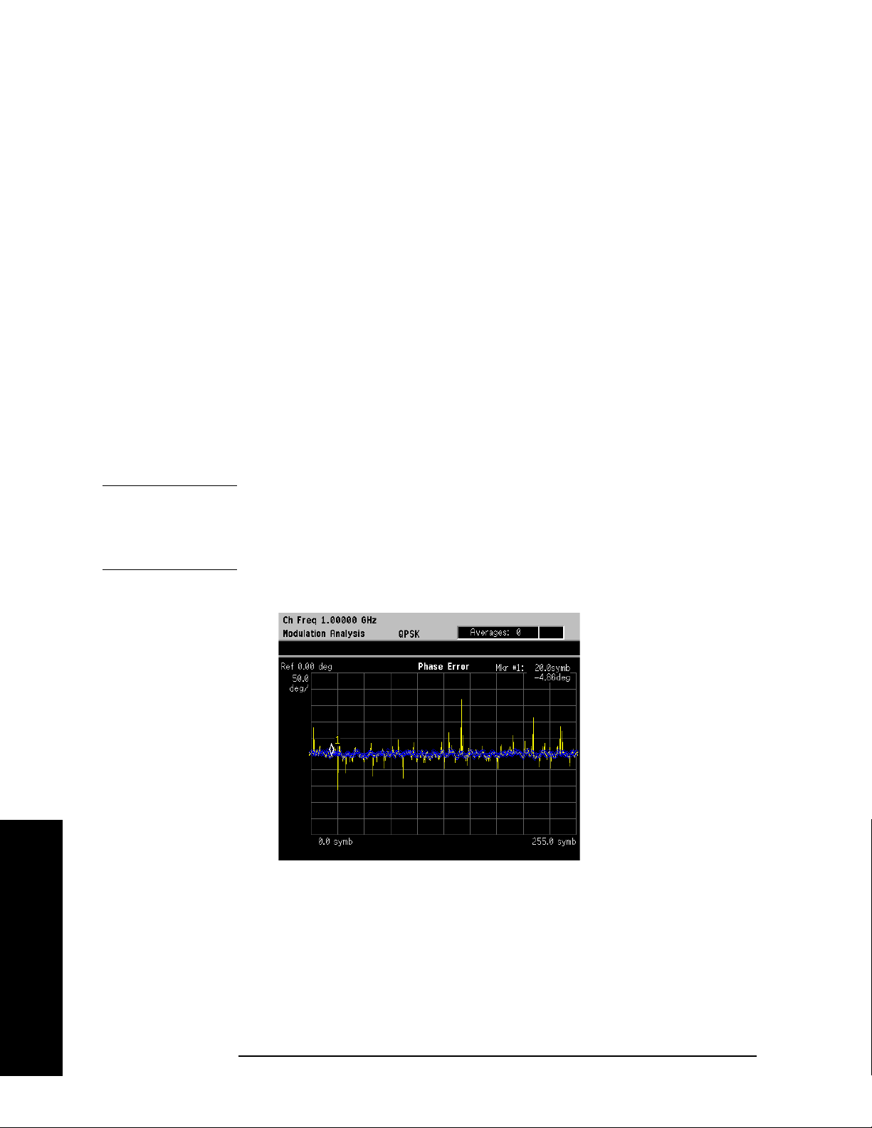
Making Measurements
Measuring Digital Modulation Formats
Viewing the Phase Error Versus Time Results
This procedure shows you how to adjust x-axis and y-axis settings for
the phase error versus time graph. By zooming into a time capture area
of interest, modulation phase errors can be identified easier.
If you have a problem, and get an error message, see “Interpreting
Error Codes” on page 119.
Step 1. Follow the procedure “Setting up the Modulation Analysis Personality”
on page 63 before continuing.
Step 2. View the I/Q error quad-view (see Figure 2-20):
Press
Trace/View, I/Q Error (Quad-View).
Step 3. View the zoomed in graph of phase error versus symbol. Use markers to
look at the phase error of individual symbol points.
Press
Press
Press
NOTE Using the Next Window key, you can scroll through the measurement
Next Window until the Phase Error window is selected.
Zoom.
Marker, Trace, Phase Error.
displays, where the current selection is highlighted with a green box
outline. The
Zoom key will zoom in on the currently selected display. To
go back to the quad-view display press Zoom again.
Figure 2-24 I/Q Error: Phase Error versus Symbol
Making Measurements
The Phase Error measurement display shows the phase error versus
symbol. Depending on the number of symbols captured in the
Interval
symbols 0 through 1 minus the
70 Chapter 2
key, by measurement default parameters, the x-axis displays
Meas Interval
Meas
Page 71

Making Measurements
Measuring Digital Modulation Formats
Step 4. Change the x-axis settings to zoom in on smaller portion of the
measurement capture interval:
Press
SPAN X Scale, Scale/Div, 3, Symbols.
To place the symbol points on the vertical graticules, use integer symbol
values for
reduce the measurement interval with the
Scale/Div. An alternate method to view less symbols is to
Meas Interval key. If you want
to view another portion of the time capture interval, adjust the
Val ue
.
Figure 2-25 I/Q Error: Phase Error versus Symbol (X-Axis Settings)
The Phase Error measurement displayed in Figure 2-25 shows an
x-axis
Scale/Div of 3 with a measurement capture interval of 256
symbols.
Ref
Step 5. Decrease the y-axis settings to increase the resolution of the phase
error results. Use the same x-axis settings from the previous step.
Press
AMPLITUDE Y Scale, Scale/Div, 20, Degrees.
Figure 2-26 I/Q Error: Phase Error versus Symbol (Y-Axis Settings)
The Phase Error measurement displayed in Figure 2-26 shows a y-axis
Making Measurements
Chapter 2 71
Page 72

Making Measurements
Measuring Digital Modulation Formats
Scale/Div of 20 degrees and a reference level of 0 degrees.
Making Measurements
72 Chapter 2
Page 73

Making Measurements
Measuring Digital Modulation Formats
Viewing the EVM Versus Time Results
This procedure shows you how to adjust x-axis and y-axis settings for
the EVM versus time graph. By zooming into a time capture area of
interest, EVM results can be analyzed at the symbol level.
If you have a problem, and get an error message, see “Interpreting
Error Codes” on page 119.
Step 1. Follow the procedure “Setting up the Modulation Analysis Personality”
on page 63 before continuing.
Step 2. View the I/Q error quad-view (see Figure 2-20):
Press
Trace/View, I/Q Error (Quad-View).
Step 3. View the zoomed in graph of EVM versus symbol. Use markers to look
at the EVM of individual symbol points.
Press
Press
Press
NOTE Using the Next Window key, you can scroll through the measurement
Next Window until the EVM window is selected.
Zoom.
Marker, Trace, EVM.
displays, where the current selection is highlighted with a green box
outline. The
Zoom key will zoom in on the currently selected display. To
go back to the quad-view display press Zoom again.
Figure 2-27 I/Q Error: EVM versus Symbol
The EVM measurement display shows EVM versus symbol. Depending
on the number of symbols captured in the
Meas Interval key, by
measurement default parameters, the x-axis displays symbols 0
through 1 minus the
Chapter 2 73
Meas Interval
Making Measurements
Page 74
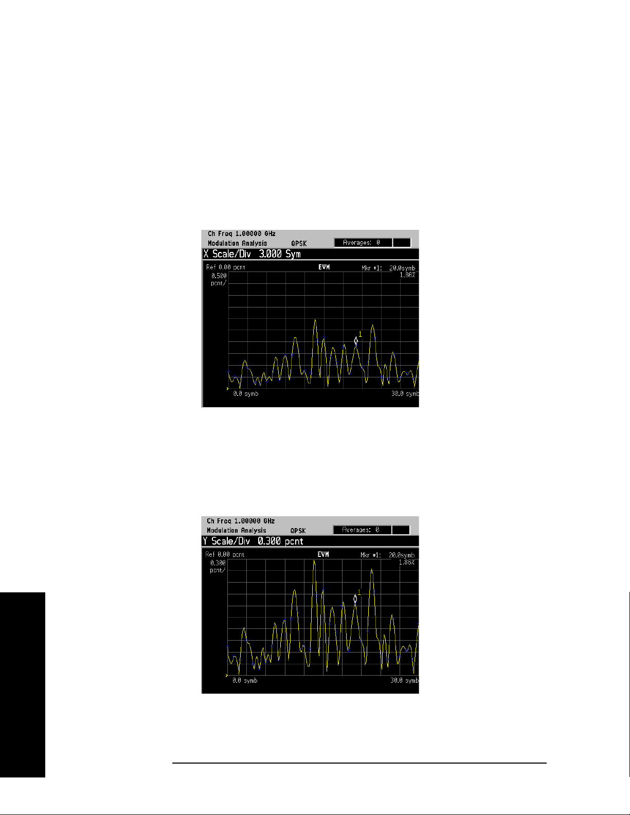
Making Measurements
Measuring Digital Modulation Formats
Step 4. Change the x-axis settings to zoom in on smaller portion of the
measurement capture interval:
Press
SPAN X Scale, Scale/Div, 3, Symbols.
To place the symbol points on the vertical graticules, use integer symbol
values for
reduce the measurement interval with the
Scale/Div. An alternate method to view less symbols is to
Meas Interval key. If you want
to view another portion of the time capture interval, adjust the
Val ue
.
Figure 2-28 I/Q Error: EVM versus Symbol (X-Axis Settings)
The EVM measurement displayed in Figure 2-28 shows an x-axis
Scale/Div of 3 with a measurement capture interval of 256 symbols.
Ref
Making Measurements
Step 5. Decrease the y-axis settings to increase the resolution of the phase
error results. Use the same x-axis settings from the previous step.
Press
AMPLITUDE Y Scale, Scale/Div, 0.3, %.
Figure 2-29 I/Q Error: EVM versus Symbol (Y-Axis Settings)
The EVM measurement displayed in Figure 2-29 shows a y-axis
Scale/Div
of 0.3 percent and a reference level of 0 percent.
74 Chapter 2
Page 75

Making Measurements
Measuring Digital Modulation Formats
Viewing the Eye Diagram Results
This procedure demonstrates the different views of the eye quad-view.
The eye quad-view allows you to view the eye I diagram, the eye Q
diagram, I/Q measured polar vector graph and a numeric results
summary table all on one screen to quickly determine any impairments
that may exist. You can zoom in on each of the 4 views for more
resolution to help pin-point any problems.
If you have a problem, and get an error message, see “Interpreting
Error Codes” on page 119.
Step 1. Follow the procedure “Setting up the Modulation Analysis Personality”
on page 63 before continuing.
Step 2. View the eye graphical results on a quad-view display.
Press
Trace/View, Eye (Quad-View).
Figure 2-30 Eye (Quad-View)
The eye quad-view measurement result displays two eye diagrams (I
and Q). The I and Q eye diagrams show the transitions of constellation
points of the QPSK signal. The eye diagrams are a continuous plot of
the symbol transitions. The eye diagram has three symbol transitions,
where the third symbol transition wraps around to the start of the eye
diagram (first symbol point on the eye diagram).
Step 3. View the zoomed in eye I diagram. Make sure the green outline is
highlighting the eye I diagram and zoom into the diagram.
Press
NOTE Using the Next Window key, you can scroll through the measurement
Zoom.
displays, where the current selection is highlighted with a green box
outline. The
Zoom key will zoom in on the currently selected display. To
go back to the quad-view display press Zoom again.
Chapter 2 75
Making Measurements
Page 76

Making Measurements
Measuring Digital Modulation Formats
Figure 2-31 Eye I Diagram
The Eye I Diagram shows the symbol transitions of the baseband I
data. The Eye Q diagram is identical to the Eye I diagram except the
symbol data from Q is offset 90 degrees from I.
Step 4. Change the scaling of the eye diagram:
Press
AMPLITUDE Y Scale, Scale/Div.
Rotate front-panel knob clockwise to increase the scale/div value.
Step 5. Pause the measurement and build the eye diagram symbol-by-symbol:
Press
Press
Meas Control, Pause.
Display, I/Q Points, 0, Enter.
Rotate front-panel knob clockwise to add symbol points.
Figure 2-32 Eye I Diagram - Building Symbol-by-Symbol
Making Measurements
In Figure 2-32, the first 5 symbols are plotted, starting with symbol 1
on the far left-side of the diagram.
NOTE The I/Q measured polar vector graph can be built the same way.
Press Meas Control, Resume to continue.
76 Chapter 2
Page 77

Making Measurements
Measuring Digital Modulation Formats
Viewing the FSK Error (Quad-View) Results
This procedure demonstrates the FSK error quad-view display. The
FSK error quad-view allows you to see the FSK error versus time, FSK
error spectrum, FSK measured time and a numeric summary table all
on one screen to quickly determine any impairments that may exist.
You can zoom in on each of the 4 views for more resolution to help
pin-point any problems.
NOTE In this procedure, a bursted Bluetooth 2-level FSK signal is used with a
symbol rate of 1 Msps, and a filter alpha of 0.5 at 1 GHz.
If you have a problem, and get an error message, see “Interpreting
Error Codes” on page 119.
Step 1. Preset the instrument and select the digital modulation personality:
Press
Press
Preset, Factory Preset (if available).
MODE, Digital Modulation.
Step 2. Select the Bluetooth pre-set radio standard and base station device:
Press
Press
Mode Setup, Radio, Radio Standard, More, Bluetooth.
Device (BTS), to underline BTS.
Step 3. Set the center frequency to 1 GHz.
Press
FREQUENCY Channel, Center Freq, 1, GHz.
Step 4. Enable the modulation analysis mode to measure and display EVM and
other modulation metrics.
Press
MEASURE, Modulation Analysis.
Step 5. Set the trigger source to capture the burst:
Press
Press
Meas Setup, Trig Source, RF Burst (Wideband).
Meas Control, Restart.
Figure 2-33 I/Q Measured Polar Graph
Chapter 2 77
Making Measurements
Page 78

Making Measurements
Measuring Digital Modulation Formats
The default view for the modulation analysis personality is the I/Q
Measured Polar Vector graph (see Figure 2-33).
Step 6. View the FSK error quad-view:
Press
Trace/View, FSK Error (Quad-View).
Figure 2-34 FSK Error (Quad-View)
The FSK error quad-view measurement result displays three graphs
and one numeric results summary table. The graphs consist of FSK
Error versus symbol, FSK Error Spectrum and FSK Meas Time. The
numerical results table shows key modulation metrics as maximum and
average values associated with the last demodulated capture period.
Making Measurements
NOTE Using the Next Window key, you can scroll through the measurement
displays, where the current selection is highlighted with a green box
outline. The
Zoom key will zoom in on the currently selected display. To
go back to the quad-view display press Zoom again.
78 Chapter 2
Page 79

Making Measurements
Measuring Digital Modulation Formats
Viewing the FSK Error Versus Time Results
This procedure shows you how to adjust x-axis and y-axis settings for
the FSK error versus time graph. By zooming into a time capture area
of interest, the FSK error results can be analyzed at the symbol level.
NOTE In this procedure, a bursted Bluetooth 2-level FSK signal is used with a
symbol rate of 1 Msps, and a filter alpha of 0.5 at 1 GHz.
If you have a problem, and get an error message, see “Interpreting
Error Codes” on page 119.
Step 1. Follow steps 1 through 5 in the procedure “Viewing the FSK Error
(Quad-View) Results” on page 77 before continuing.
Step 2. View the FSK error quad-view (see Figure 2-34):
Press
Trace/View, FSK Error (Quad-View).
Step 3. View the zoomed in graph of FSK error versus symbol. Use markers to
look at the error of individual symbol points.
Press
Press
Zoom.
Marker, Trace, FSK Error. then use the numeric keypad or
front-panel knob to place the marker on a symbol.
NOTE Using the Next Window key, you can scroll through the measurement
displays, where the current selection is highlighted with a green box
outline. The
Zoom key will zoom in on the currently selected display. To
go back to the quad-view display press Zoom again.
Figure 2-35 FSK Error versus Symbol
The FSK error measurement display shows FSK error versus symbol.
Depending on the number of symbols captured in the
Meas Interval key,
by measurement default parameters, the x-axis displays symbols 0
through 1 minus the
Chapter 2 79
Meas Interval
Making Measurements
Page 80

Making Measurements
Measuring Digital Modulation Formats
Step 4. Change the x-axis settings to zoom in on smaller portion of the
measurement capture interval:
Press
SPAN X Scale, Scale/Div, 3, Symbols.
To place the symbol points on the vertical graticules, use integer symbol
values for
reduce the measurement interval with the
Scale/Div. An alternate method to view less symbols is to
Meas Interval key. If you want
to view another portion of the time capture interval, adjust the
Val ue
.
Figure 2-36 FSK Error versus Symbol (X-Axis Settings)
Ref
Making Measurements
The FSK error measurement displayed in Figure 2-36 shows an x-axis
Scale/Div of 3 with a measurement capture interval of 256 symbols.
Step 5. Decrease the y-axis settings to increase the resolution of the FSK error
results. Use the same x-axis settings from the previous step.
Press
AMPLITUDE Y Scale, Scale/Div, 0.2, %.
Figure 2-37 FSK Error versus Symbol (Y-Axis Settings)
The FSK Error measurement displayed in Figure 2-37 shows a y-axis
Scale/Div
of 0.2 percent and a reference level of 0 percent.
80 Chapter 2
Page 81
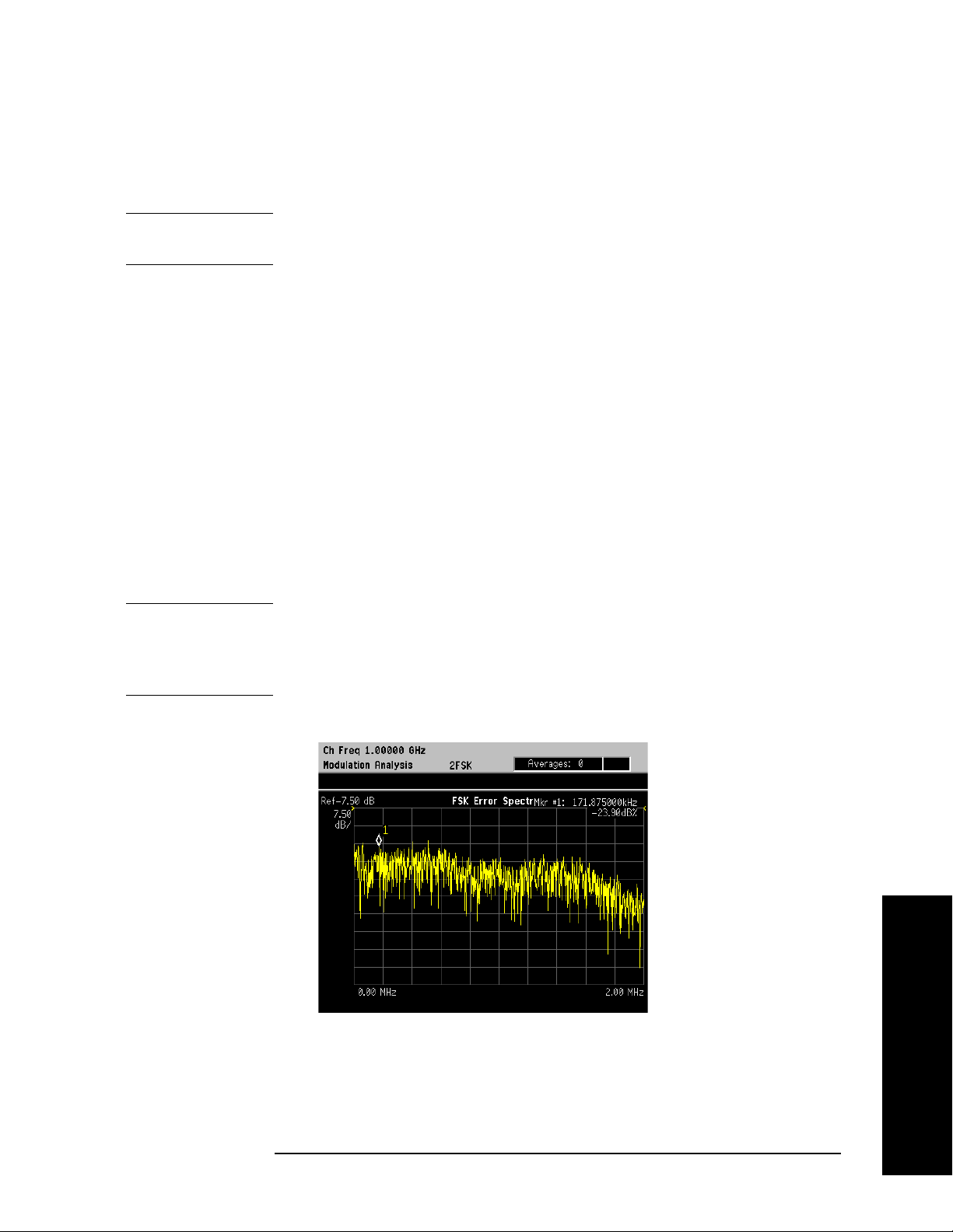
Making Measurements
Measuring Digital Modulation Formats
Viewing the FSK Error Spectrum Results
This procedure shows you how to adjust x-axis and y-axis settings for
the FSK error spectrum graph.
NOTE In this procedure, a bursted Bluetooth 2-level FSK signal is used with a
symbol rate of 1 Msps, and a filter alpha of 0.5 at 1 GHz.
If you have a problem, and get an error message, see “Interpreting
Error Codes” on page 119.
Step 1. Follow steps 1 through 5 in the procedure “Viewing the FSK Error
(Quad-View) Results” on page 77 before continuing.
Step 2. View the FSK error quad-view (see Figure 2-34):
Press
Trace/View, FSK Error (Quad-View).
Step 3. View the zoomed in graph of FSK error spectrum. Use markers to look
at frequency points of the error spectrum.
Press
Press
Press
Next Window until the FSK error spectrum graph is selected.
Zoom.
Marker, Trace , FSK Error Spectrum, then use the numeric keypad or
front-panel knob to place the marker on a frequency point.
NOTE Using the Next Window key, you can scroll through the measurement
displays, where the current selection is highlighted with a green box
outline. The
Zoom key will zoom in on the currently selected display. To
go back to the quad-view display press Zoom again.
Figure 2-38 FSK Error Spectrum
When you select FSK error spectrum, the analyzer displays the
spectrum of FSK error versus time. In other words, the analyzer derives
the FSK error time trace, and then windows and FFTs this trace to
produce the FSK error spectrum trace.
Chapter 2 81
Making Measurements
Page 82

Making Measurements
Measuring Digital Modulation Formats
Step 4. Change the x-axis settings to zoom in on smaller portion of the error
spectrum:
Press
SPAN X Scale, Scale/Div, 20, kHz.
Figure 2-39 FSK Error Spectrum (X-Axis Settings)
The FSK Error Spectrum measurement displayed in Figure 2-39
shows an x-axis
Scale/Div of 20 kHz.
Step 5. Decrease the y-axis settings to increase the resolution of the FSK error
spectrum results. Use the same x-axis settings from the previous step.
Press
AMPLITUDE Y Scale, Scale/Div, 5, dB.
Making Measurements
Figure 2-40 FSK Error Spectrum (Y-Axis Settings)
The FSK Error Spectrum measurement displayed in Figure 2-40
shows a y-axis
Scale/Div of 5 dB and a reference level of −7.5 dB.
82 Chapter 2
Page 83
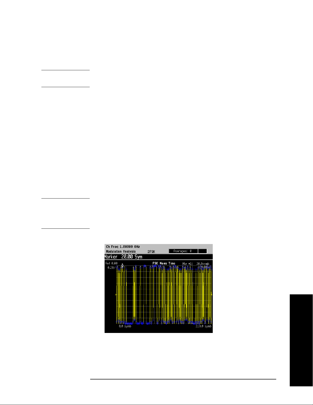
Making Measurements
Measuring Digital Modulation Formats
Viewing the FSK Measured Time Results
This procedure shows you how to adjust x-axis and y-axis settings for
the FSK measured time graph.
NOTE In this procedure, a bursted Bluetooth 2-level FSK signal is used with a
symbol rate of 1 Msps, and a filter alpha of 0.5 at 1 GHz.
If you have a problem, and get an error message, see “Interpreting
Error Codes” on page 119.
Step 1. Follow steps 1 through 5 in the procedure “Viewing the FSK Error
(Quad-View) Results” on page 77 before continuing.
Step 2. View the FSK error quad-view (see Figure 2-34):
Press
Trace/View, FSK Error (Quad-View).
Step 3. View the zoomed in graph of FSK measured time. Use markers to look
at the measured symbol points.
Press
Press
Press
Next Window until the FSK measured time graph is selected.
Zoom.
Marker, Trace, FSK Measured, then use the numeric keypad or
front-panel knob to place the marker on a symbol.
NOTE Using the Next Window key, you can scroll through the measurement
displays, where the current selection is highlighted with a green box
outline. The
Zoom key will zoom in on the currently selected display. To
go back to the quad-view display press Zoom again.
Figure 2-41 FSK Measured Time
The FSK measured time display shows the symbol decision points
versus time. Depending on the number of symbols captured in the
Interval
symbols 0 through 1 minus the
Chapter 2 83
key, by measurement default parameters, the x-axis displays
Meas Interval
Meas
Making Measurements
Page 84

Making Measurements
Measuring Digital Modulation Formats
Step 4. Change the x-axis settings to zoom in on smaller portion of the
measurement capture interval:
Press
SPAN X Scale, Scale/Div, 3, Symbols.
To place the symbol points on the vertical graticules, use integer symbol
values for
Scale/Div. An alternate method to view less symbols is to
reduce the measurement interval with the
to view another portion of the time capture interval, adjust the
Val ue
.
Figure 2-42 FSK Measured Time (X-Axis Settings)
Meas Interval key. If you want
Ref
Making Measurements
The FSK Meas Time display in Figure 2-42 shows an x-axis
3 symbols per division with a measurement interval of 320 symbols.
Step 5. Increase the y-axis settings to observe how y-axis scaling works. Use
the same x-axis settings from the previous step.
Press
AMPLITUDE Y Scale, Scale/Div, 0.3, Enter.
Figure 2-43 FSK Measured Time (Y-Axis Settings)
The FSK Measured Time display in Figure 2-43 shows a y-axis
of 0.3 and a reference value of 0.
Scale/Div of
Scale/Div
84 Chapter 2
Page 85

Making Measurements
Measuring Digital Modulation Formats
PSK Modulation Analysis (cdma2000 QPSK Example)
Supported PSK formats: BPSK, QPSK, 8PSK, DQPSK, D8PSK, Pi/4
DQPSK and Offset QPSK.
This section explains how to demodulate and analyze a cdma2000
signal (pilot channel only) at 1 GHz and −10 dBm. This measurement
procedure guides you through the different measurement views useful
for modulation analysis.
Configuring the Measurement System
Refer to “Configuring a BTS Measurement System” on page 29 to
connect the measurement equipment.
Measurement Procedure
If you have a problem, and get an error message, see “Interpreting
Error Codes” on page 119.
Step 1. Preset the instrument and select the digital modulation personality:
Press
Press
Preset, Factory Preset (if available).
MODE, Digital Modulation.
Step 2. Select the cdma2000 radio standard pre-set and base station device:
Press
Press
Mode Setup, Radio, Radio Standard, cdma2000.
Device (BTS), to underline BTS.
Step 3. Enable the modulation analysis mode to measure and display EVM and
other modulation metrics.
Press
MEASURE, Modulation Analysis.
Figure 2-44 I/Q Measured Polar Vector Graph (Default View)
Making Measurements
The measurement values for EVM, magnitude error, phase error,
frequency error, I/Q offset and rho are shown in the summary window
on the left side of the display.
Chapter 2 85
Page 86

Making Measurements
Measuring Digital Modulation Formats
Step 4. View the I/Q error quad-view display to view the magnitude and phase
error components versus time and EVM versus time to quickly
pin-point possible modulation problems:
Press
Trace/View, I/Q Error (Quad-View).
Figure 2-45 I/Q Error (Quad-View)
Step 5. View the eye quad-view display to quickly determine if the eye I and
eye Q diagrams are symmetrical with good symbol transitions.
Press
Trace/View, Eye (Quad-View).
Figure 2-46 Eye (Quad-View)
Making Measurements
86 Chapter 2
Page 87

Making Measurements
Measuring Digital Modulation Formats
QAM Modulation Analysis (64QAM Example)
Supported QAM formats: 16QAM, 32QAM, 64QAM, 128QAM and
256QAM.
This section explains how to demodulate and analyze a 64QAM signal
at 1 GHz, −10 dBm with a root nyquist filter alpha of 0.25 and a symbol
rate of 5 Msps. This measurement procedure guides you through the
different measurement views useful for modulation analysis.
Measurement Procedure
If you have a problem, and get an error message, see “Interpreting
Error Codes” on page 119.
Step 1. Preset the instrument and select the digital modulation personality:
Press
Press
Press
Preset, Factory Preset (if available).
MODE, Digital Modulation.
MEASURE, Modulation Analysis.
Step 2. Modify the demodulation parameters:
Press
Press
Press
Press
Press
Press
Meas Setup, Demod.
Modulation Format, More, 64QAM.
Meas Filter, Root Nyquist.
Ref Filter, Nyquist.
Alpha/BT, 0.25, Enter.
Symbol Rate, 5, MHz.
Figure 2-47 I/Q Measured Polar Vector Graph (Default View)
The measurement values for EVM, magnitude error, phase error,
frequency error, I/Q offset and rho are shown in the summary window
on the left side of the display.
Chapter 2 87
Making Measurements
Page 88

Making Measurements
Measuring Digital Modulation Formats
Step 3. View the I/Q error quad-view display to view the magnitude and phase
error components versus time and EVM versus time to quickly
pin-point possible modulation problems:
Press
Trace/View, I/Q Error (Quad-View).
Figure 2-48 I/Q Error (Quad-View)
Step 4. View the eye quad-view display to quickly determine if the eye I and
eye Q diagrams are symmetrical with good symbol transitions.
Press
Trace/View, Eye (Quad-View).
Figure 2-49 Eye (Quad-View)
Making Measurements
88 Chapter 2
Page 89
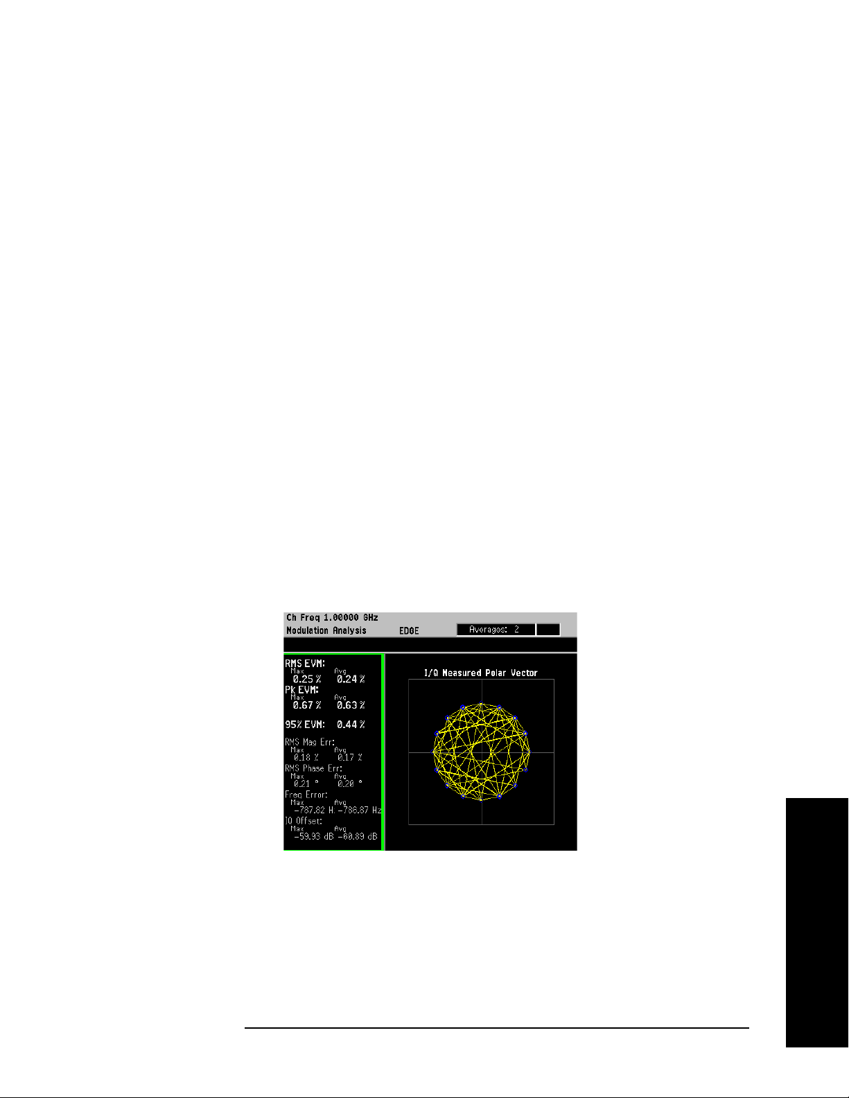
Making Measurements
Measuring Digital Modulation Formats
EDGE Modulation Analysis
This section explains how to demodulate and analyze an EDGE signal
at 1 GHz, −10 dBm. This measurement procedure guides you through
the different measurement views useful for modulation analysis.
Configuring the Measurement System
Refer to “Configuring a BTS Measurement System” on page 29 to
connect the measurement equipment.
Measurement Procedure
If you have a problem, and get an error message, see “Interpreting
Error Codes” on page 119.
Step 1. Preset the instrument and select the digital modulation personality:
Press
Press
Preset, Factory Preset (if available).
MODE, Digital Modulation.
Step 2. Select the EDGE radio standard pre-set and base station device:
Press
Press
Mode Setup, Radio, Radio Standard, EDGE.
Device (BTS), to underline BTS.
Step 3. Enable the modulation analysis mode to measure and display EVM and
other modulation metrics.
Press
MEASURE, Modulation Analysis.
Figure 2-50 I/Q Measured Polar Vector Graph (Default View)
The measurement values for EVM, magnitude error, phase error,
frequency error, I/Q offset and rho are shown in the summary window
on the left side of the display.
Chapter 2 89
Making Measurements
Page 90
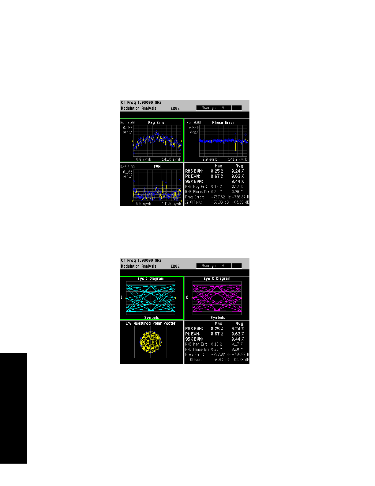
Making Measurements
Measuring Digital Modulation Formats
Step 4. View the I/Q error quad-view display to view the magnitude and phase
error components versus time and EVM versus time to quickly
pin-point possible modulation problems:
Press
Trace/View, I/Q Error (Quad-View).
Figure 2-51 I/Q Error (Quad-View)
Step 5. View the eye quad-view display to quickly determine if the eye I and
eye Q diagrams are symmetrical with good symbol transitions.
Press
Trace/View, Eye (Quad-View).
Figure 2-52 Eye (Quad-View)
Making Measurements
90 Chapter 2
Page 91
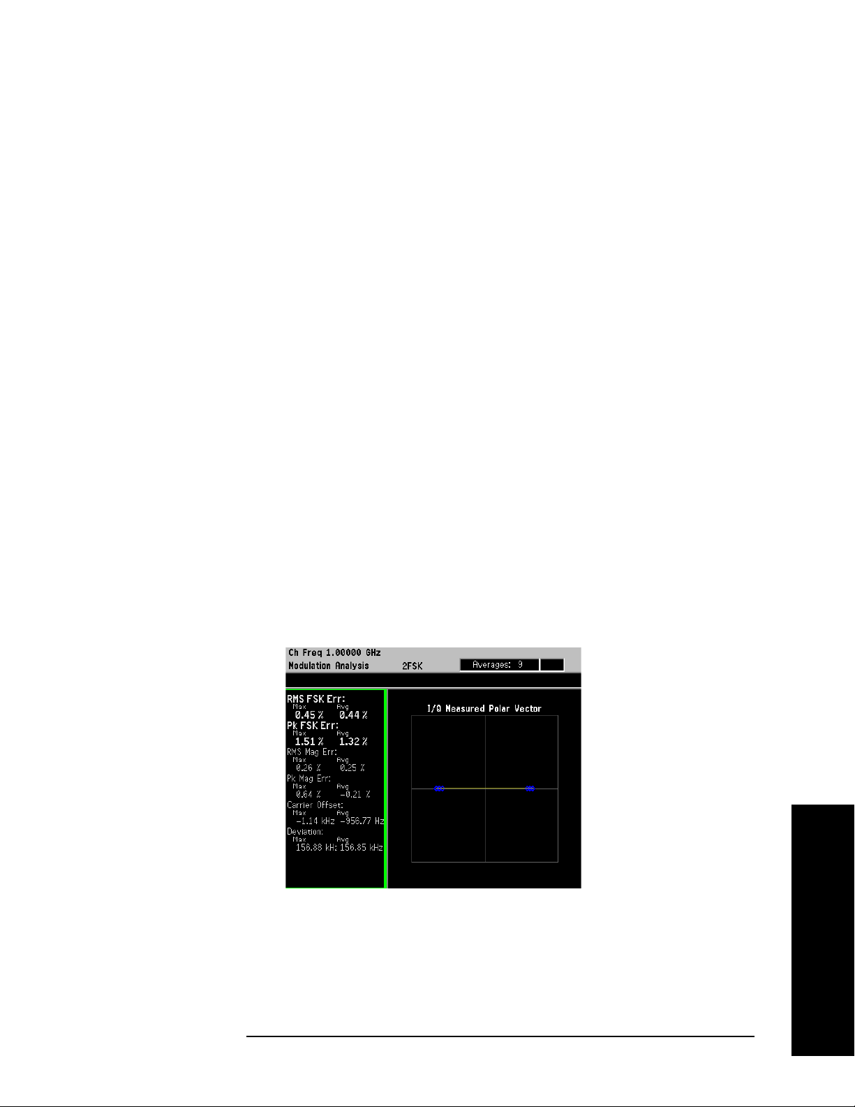
Making Measurements
Measuring Digital Modulation Formats
FSK Modulation Analysis (Bluetooth 2FSK Example)
Supported FSK formats: 2FSK, 4FSK and 8FSK.
This section explains how to demodulate and analyze a bursted
Bluetooth signal at 1 GHz, −10 dBm. This measurement procedure
guides you through the different measurement views useful for
modulation analysis.
Measurement Procedure
If you have a problem, and get an error message, see “Interpreting
Error Codes” on page 119.
Step 1. Preset the instrument and select the digital modulation personality:
Press
Press
Preset, Factory Preset (if available).
MODE, Digital Modulation.
Step 2. Select the Bluetooth radio standard pre-set:
Press
Mode Setup, Radio, Radio Standard, More, Bluetooth.
Step 3. Enable the modulation analysis mode to measure and display EVM and
other modulation metrics.
Press
MEASURE, Modulation Analysis.
Step 4. Set the trigger source to capture the Bluetooth burst:
Press
Press
Meas Setup, Trig Source, RF Burst (Wideband).
Meas Control, Restart.
Figure 2-53 I/Q Measured Polar Vector Graph (Default View)
In Figure 2-53, the measurement values for FSK error, magnitude
error, carrier offset and deviation are shown in the summary window on
the left side of the display.
Chapter 2 91
Making Measurements
Page 92

Making Measurements
Measuring Digital Modulation Formats
Step 5. View the FSK error quad-view display:
Press
Trace/View, FSK Error (Quad-View).
The FSK error quad-view display contains FSK error versus time, FSK
error spectrum, FSK measured time and a numeric summary table. You
can zoom in on any of these views for better resolution.
Figure 2-54 FSK Error (Quad-View)
Step 6. View the numeric results table to quickly determine where problems
might exist in the modulation.
Press
Trace/View, Numeric Results.
Figure 2-55 FSK Numeric Results
Making Measurements
92 Chapter 2
Page 93

Making Measurements
Measuring Digital Modulation Formats
MSK Modulation Analysis (GSM MSK type 1 Example)
Supported MSK formats: MSK type 1 and MSK type 2.
This section explains how to demodulate and analyze a GSM signal at 1
GHz and −10 dBm. This measurement procedure guides you through
the different measurement views useful for modulation analysis.
Configuring the Measurement System
Refer to “Configuring a BTS Measurement System” on page 29 to
connect the measurement equipment.
Measurement Procedure
If you have a problem, and get an error message, see “Interpreting
Error Codes” on page 119.
Step 1. Preset the instrument and select the digital modulation personality:
Press
Press
Preset, Factory Preset (if available).
MODE, Digital Modulation.
Step 2. Select the GSM radio standard pre-set and base station device:
Press
Press
Mode Setup, Radio, Radio Standard, GSM.
Device (BTS), to underline BTS.
Step 3. Enable the modulation analysis mode to measure and display EVM and
other modulation metrics.
Press
MEASURE, Modulation Analysis.
Figure 2-56 I/Q Measured Polar Vector Graph (Default View)
The measurement values for EVM, magnitude error, phase error,
frequency error and I/Q offset are shown in the summary window on the
left side of the display.
Chapter 2 93
Making Measurements
Page 94
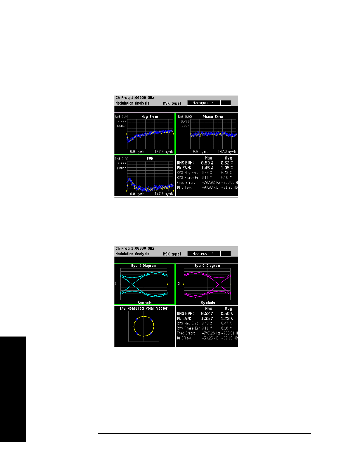
Making Measurements
Measuring Digital Modulation Formats
Step 4. View the I/Q error quad-view display to view the magnitude and phase
error components versus time and EVM versus time to quickly
pin-point possible modulation problems:
Press
Trace/View, I/Q Error (Quad-View).
Figure 2-57 I/Q Error (Quad-View)
Step 5. View the eye quad-view display to quickly determine if the eye I and
eye Q diagrams are symmetrical with good symbol transitions.
Press
Trace/View, Eye (Quad-View).
Figure 2-58 Eye (Quad-View)
Making Measurements
94 Chapter 2
Page 95

Making Measurements
Analyzing and Troubleshooting Digital Signals
Analyzing and Troubleshooting Digital Signals
EVM Troubleshooting Procedure Overview
Measurements of EVM and related quantities can pin-point the causes
of many problems uncovered during the design stages. This section
provides general guidance for troubleshooting those problems and the
techniques to determine what kind of impairments could be due to your
design or testing procedure. Figure 2-59 shows the troubleshooting
procedure to help determine the root cause of your measurement
results.
If you have high EVM results, the first step is to break the EVM result
into phase and magnitude components. With phase and magnitude
errors, you can determine whether you need to view phase error vs.
time, magnitude error vs. time or the I/Q constellation. For example, if
you determined the phase error and magnitude error add about the
same amount of error to the EVM result and the I/Q constellation is
symmetric then you should look closely at EVM vs. time.
Figure 2-59 Flow Chart for EVM Troubleshooting
Making Measurements
Chapter 2 95
Page 96

Making Measurements
Analyzing and Troubleshooting Digital Signals
Measurement 1 - Obtaining EVM Results with Phase Error and Magnitude Error
The PSA Option 241 can help design engineers pin-point signal errors
or measurement set-up errors from basic digitally modulated signals to
complex digitally modulated high data rate signals.
To demonstrate using PSA option 241 for troubleshooting signal and
set-up impairments, a W-CDMA signal is used.
Step 1. Generate a downlink (base station) W-CDMA signal with 1 data
channel (DPCH). Set the carrier frequency at 1 GHz with an amplitude
of −10 dBm. The W-CDMA signal is impairment free.
Step 2. Setup the PSA to demodulate the W-CDMA signal using option 241:
Press
Press
Press
Press
Preset, Factory Preset (if available).
MODE, Digital Modulation.
FREQUENCY Channel, Center Freq, 1, GHz.
MEASURE, Modulation Analysis.
Step 3. View the numeric results and note the average (RMS) EVM, RMS
magnitude error and RMS phase error results:
Press
Trace/View, Numeric Results.
If you have higher than expected RMS and/or peak EVM results, look at
the RMS magnitude error (number 1 in Figure 2-60) and RMS phase
error (number 2 in Figure 2-60). If the phase error is relatively larger
(greater than 3-4 times) than the magnitude error go to “Measurement
2 - Phase Error vs. Time” on page 97. If the magnitude error is
relatively larger (greater than 3-4 times) than the phase error go to
“Measurement 3 - Magnitude Error vs. Time” on page 98. If the phase
error and magnitude error are approximately the same go to
“Measurement 4 - I/Q Constellation Diagram” on page 99.
Figure 2-60 Numeric Results (comparing phase and magnitude errors)
not
similar
Making Measurements
96 Chapter 2
Page 97

Analyzing and Troubleshooting Digital Signals
Measurement 2 - Phase Error vs. Time
Measurement procedure: use if phase error >> magnitude error.
Description: Phase error is the instantaneous angle difference between
the measured signal and the ideal reference signal. When viewed as a
function of time (or symbol), it shows the modulating waveform of any
residual or interfering PM signal.
Step 1. Display the phase error versus time (symbols) results:
Making Measurements
Press
Press
Trace/View, I/Q Error (Quad-View).
Next Window, Zoom.
The full screen view should now be the phase error diagram.
Step 2. Adjust the vertical scale as necessary to view the phase error:
Press
By manually changing the
are not sure what
AMPLITUDE Y Scale, Scale/Div then adjust as necessary.
Scale/Div, the Scale Coupling turns off. If you
Scale/Div to use, set Scale Coupling to on.
Step 3. For more detail, expand the waveform by reducing the result length or
by reducing the x-scale per division.
Press
Press
Meas Setup, Demod, Meas Interval, or
SPAN X Scale, Scale/Div, then adjust the measurement interval or
x-axis as necessary.
TIP The x-axis scale is in symbols. To calculate absolute time, divide the
number of symbols by the symbol rate.
Observe: Sine waves or other regular waveforms indicate an interfering
signal. See “In-Channel Phase Modulating (PM) Interference” on
page 107 for an example of residual PM. Uniform noise is a sign of some
form of phase noise (i.e. random jitter). See Figure 2-61 for an example.
Figure 2-61 Phase Error Zoom View - Example of Uniform Noise
Chapter 2 97
Making Measurements
Page 98

Making Measurements
Analyzing and Troubleshooting Digital Signals
Measurement 3 - Magnitude Error vs. Time
Measurement procedure: use if phase error << magnitude error.
Description: Magnitude error is the instantaneous amplitude difference
between the measured signal and the ideal reference signal. When
viewed as a function of time (or symbol), it shows the modulating
waveform of any residual or interfering AM signal.
Step 1. Display the magnitude error versus time (symbols) results:
Press
Trace/View, I/Q Error (Quad-View). (Confirm the current selected
view is Mag Error. The current selection is outlined in green.)
Press
NOTE If you need to go back to the quad-view, press Zoom one more time.
Zoom.
The full screen view should now be the magnitude error diagram.
Step 2. Adjust the vertical scale as necessary to view the magnitude error:
Press
By manually changing the
are not sure what
AMPLITUDE Y Scale, Scale/Div then adjust as necessary.
Scale/Div, the Scale Coupling turns off. If you
Scale/Div to use, set Scale Coupling to on.
Step 3. For more detail, expand the waveform by reducing the result length or
by reducing the x-scale per division.
Press
Press
Meas Setup, Demod, Meas Interval, or
SPAN X Scale, Scale/Div, then adjust the measurement interval or
x-axis as necessary.
If magnitude error versus time shows a curve response then amplitude
droop could be the problem. If you see a waveform pattern then residual
AM could be the problem. See “In-Channel Amplitude Modulation (AM)
Interference” on page 109 for an example of residual AM.
Making Measurements
Figure 2-62 Magnitude Error Zoom View - Example of Uniform Noise
98 Chapter 2
Page 99

Making Measurements
Analyzing and Troubleshooting Digital Signals
Measurement 4 - I/Q Constellation Diagram
Measurement procedure: use if phase error ≅ magnitude error.
Description: This is a common graphical analysis technique utilizing a
polar plot to display a vector-modulated signal’s magnitude and phase
relative to the carrier, as a function of time or symbol. The phasor
values at the symbol clock times are particularly important, and are
highlighted with a dot (at a symbol point). In order to accomplish this, a
constellation analyzer must know the precise carrier and symbol clock
frequencies and phases, either through an external input or through
automatic locking, as with PSA Option 241.
Step 1. Display the I/Q measured time polar constellation graph (default view):
Press
Trace/View, I/Q Measured Polar Graph.
The individual constellation “dots” represent the modulation symbol
states. The lines connecting the states are the signal “trajectories” for
the phase and amplitude of the modulation between symbols.
Step 2. Adjust the number of I/Q points displayed in the constellation view:
Press
Display, I/Q Points.
For a constellation with a low number of symbol states, enter a number
at least several times the number of states in the constellation. That
will allow each state to clearly show the distribution of measured
symbols. If no symbol “dot” is shown, it may mean that state was not
transmitted. You may need to use random data to see all the “dots”.
TIP I/Q Points determines how many dots will appear on the constellation.
Increase it to populate the constellation states more completely.
I/Q Points cannot exceed the measurement interval.
If you are examining a constellation that contains a large number of
symbol states, like 256QAM, it may become difficult to see individual
trajectories. It can be helpful to limit the number of “dots” shown by
adjusting the number of symbols displayed lower than the number of
symbol states in the constellation, and repeating the measurement to
“see” all the constellation dots and the trajectories.
Step 3. Adjust the number of points/symbol displayed in the constellation view:
Press
TIP Points/symbol determines how much detail is shown between symbols.
Display, Points/Symbol.
To see peaks and overshoot due to filter errors, use four or more
points/symbol.
To allow a longer result length, use fewer points (in either case, result
length multiplied by points/symbol must be less than max time points).
Chapter 2 99
Making Measurements
Page 100
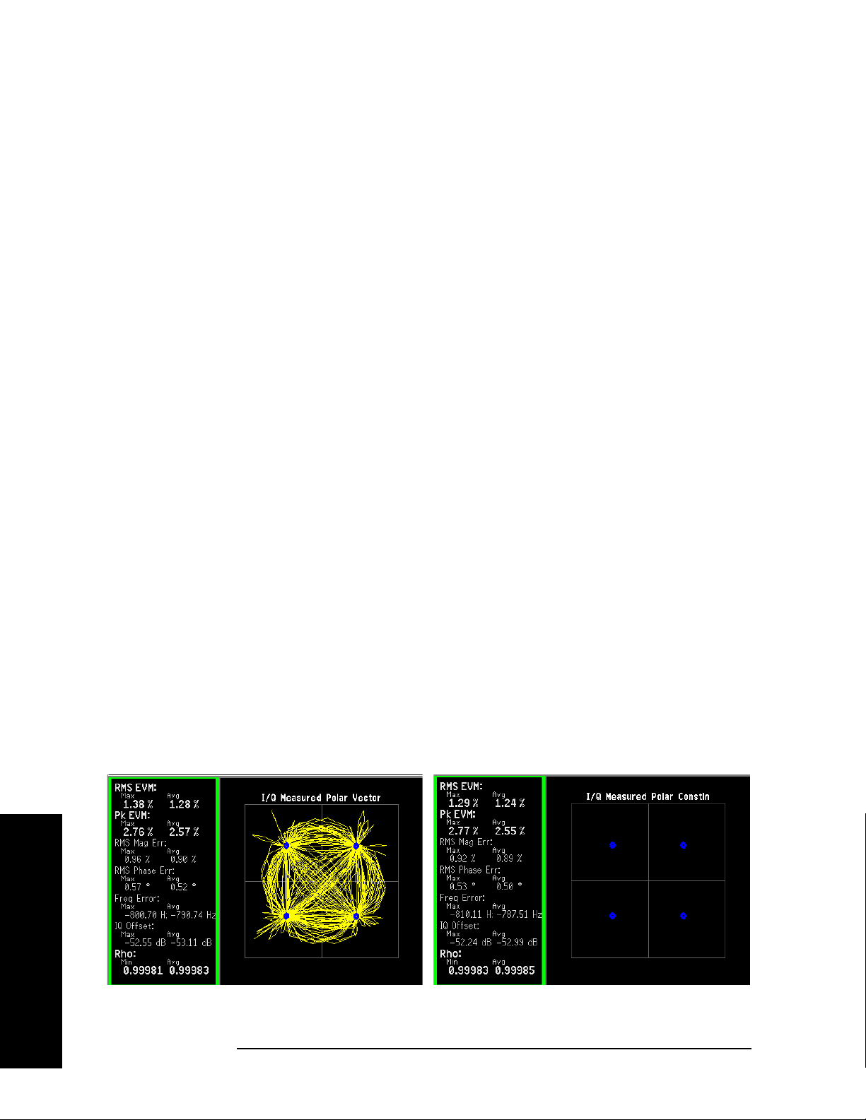
Making Measurements
Analyzing and Troubleshooting Digital Signals
One point per symbol creates misleading eye and constellation
diagrams, because no intersymbol data is collected and all symbols are
connected by straight, direct lines.
Step 4. Check the I/Q constellation for symmetry.
Observe: A perfect signal will have a uniform constellation that is
perfectly symmetric about the origin. Asymmetrical constellations fall
into the following categories:
• I/Q imbalance (“I/Q Gain Imbalance” on page 103) is indicated when
the constellation is not “square,” that is when the Q-axis height does
not equal the I-axis width.
• Quadrature error (“I/Q Quadrature Skew” on page 105) is seen as a
“tilt” to the constellation.
• I/Q offset (“I/Q DC Offset Error” on page 106) shows up as a numeric
result, since the PSA only reports the value and adjusts the
constellation to remove any offset.
Step 5. In some cases it may be easier to spot modulation problems if the
symbol trajectories are turned off:
Press
Display, I/Q Polar Type, Constellation.
Typical problems that can be easily identified by viewing the
constellation points are compression and interfering spurious signals.
Compression is the result of higher phase errors at larger signal
amplitudes.
• Interfering spur - “In-Channel Spurious Signal Interference” on
page 111 shows up as rings at the symbol points.
• Compression - symbol point shadowing effect
Step 6. If the constellation is symmetric with no abnormalities, continue to
measurement 5, to analyze EVM versus time.
Figure 2-63 I/Q Measured Polar Vector (Left) and Constellation (Right)
Making Measurements
100 Chapter 2
 Loading...