

Page 1

User’s, Programming, and Measurement Guide
Agilent Technologies
ESA-E Series Spectrum Analyzers
Modulation Analysis Measurement Personality
This guide documents firmware revision A.08.xx
This manual provides documentation for the following instruments:
Agilent ESA-E Series
E4402B (9 kHz - 3.0 GHz)
E4404B (9 kHz - 6.7 GHz)
E4405B (9 kHz - 13.2 GHz)
E4407B (9 kHz - 26.5 GHz)
Manufacturing Part Number: E4402-90071
Supersedes E4402-90037
Printed in USA
February 2002
© Copyright 2001, 2002 Agilent Technologies, Inc.
Page 2

Notice
The information contained in this document is subject to change without notice.
Agilent Technologies makes no warranty of any kind with regard to this material,
including but not limited to, the implied warranties of merchantability and fitness
for a particular purpose. Agilent Technologies shall not be liable for errors
contained herein or for incidental or consequential damages in connection with the
furnishing, performance, or use of this material.
Warranty
This Agilent Technologies instrument product is warranted against defects in
material and workmanship for a period of three years from date of shipment.
During the warranty period, Agilent Technologies Company will, at its option,
either repair or replace products that prove to be defective.
For warranty service or repair, this product must be returned to a service facility
designated by Agilent Technologies. Buyer shall prepay shipping charges to
Agilent Technologies and Agilent Technologies shall pay shipping charges to
return the product to Buyer. However, Buyer shall pay all shipping charges, duties,
and taxes for products returned to Agilent Technologies from another country.
Agilent Technologies warrants that its software and firmware designated by
Agilent Technologies for use with an instrument will execute its programming
instructions when properly installed on that instrument. Agilent Technologies does
not warrant that the operation of the instrument, or software, or firmware will be
uninterrupted or error-free.
LIMITATION OF WARRANTY
The foregoing warranty shall not apply to defects resulting from improper or
inadequate maintenance by Buyer, Buyer-supplied software or interfacing,
unauthorized modification or misuse, operation outside of the environmental
specifications for the product, or improper site preparation or maintenance.
NO OTHER WARRANTY IS EXPRESSED OR IMPLIED. AGILENT
TECHNOLOGIES SPECIFICALLY DISCLAIMS THE IMPLIED
WARRANTIES OF MERCHANTABILITY AND FITNESS FOR A
PARTICULAR PURPOSE.
2
Page 3

EXCLUSIVE REMEDIES
THE REMEDIES PROVIDED HEREIN ARE BUYER’S SOLE AND
EXCLUSIVE REMEDIES. AGILENT TECHNOLOGIES SHALL NOT BE
LIABLE FOR ANY DIRECT, INDIRECT, SPECIAL, INCIDENTAL, OR
CONSEQUENTIAL DAMAGES, WHETHER BASED ON CONTRACT, TORT,
OR ANY OTHER LEGAL THEORY.
Safety Information
The following safety notes are used throughout this manual. Familiarize yourself
with these notes before operating this instrument.
WARNING Warning denotes a hazard. It calls attention to a procedure which, if not
correctly performed or adhered to, could result in injury or loss of life. Do not
proceed beyond a warning note until the indicated conditions are fully
understood and met.
CAUTION Caution denotes a hazard. It calls attention to a procedure that, if not correctly
performed or adhered to, could result in damage to or destruction of the
instrument. Do not proceed beyond a caution sign until the indicated conditions are
fully understood and met.
WARNING This is a Safety Class 1 Product (provided with a protective earth ground
incorporated in the power cord). The mains plug shall be inserted only in a
socket outlet provided with a protected earth contact. Any interruption of the
protective conductor inside or outside of the product is likely to make the
product dangerous. Intentional interruption is prohibited.
WARNING No operator serviceable parts inside. Refer servicing to qualified personnel.
To prevent electrical shock do not remove covers.
CAUTION Always use the three-prong AC power cord supplied with this product. Failure to
ensure adequate grounding may cause product damage.
3
Page 4

4
Page 5

Contents
U
s
n
g
T
h
s
D
o
c
u
m
e
n
t
L
s
tof
C
o
m
m
a
n
d
s
T
a
b
l
e
o
f
C
o
n
t
e
n
t
s
g
1. Using This Document
BookOrganization........................................................... 16
2. Understanding Modulation Analysis
DigitalCommunicationSystemsStandardsOverview .............................. 20
ThecdmaOne(IS-95)CommunicationSystem................................... 20
TheW-CDMACommunicationSystem......................................... 20
TheCDMA2000CommunicationSystem ....................................... 20
W-CDMAandcdma2000Advantages .......................................... 20
cdmaOneStandards........................................................ 22
TheNADCCommunicationsSystem........................................... 25
TheGSMStandards........................................................ 26
TheEDGEStandard........................................................ 30
ThePDCStandard ......................................................... 32
TheTETRAStandard....................................................... 32
WhattheModulationAnalysisMeasurementPersonalityDoes....................... 33
OtherSourcesofMeasurementInformation ...................................... 36
3. Getting Started
InstrumentOverview......................................................... 38
Front-PanelFeatures ....................................................... 38
Rear-PanelFeatures........................................................ 39
OptionsRequired............................................................ 41
Installing Optional Measurement Personalities . . . ................................ 43
ActiveLicenseKey ......................................................... 43
Installing the Licensing Key ................................................. 43
UsingtheInstallKey ....................................................... 44
InstallerScreenandMenu................................................... 47
AgilentESASpectrumAnalyzersUpdate....................................... 48
4. Setting Up the Modulation Analysis Mode
PreparingtoMakeMeasurements .............................................. 50
InitialSettings ............................................................ 50
HowtoMakeanEVM(ErrorVectorMagnitude)Measurement..................... 51
HowtoSaveMeasurementResults............................................ 52
5. Making Modulation Analysis Measurements
WhatYouWillFindinThisChapter.............................................54
TheModulationAnalysisPersonality............................................ 55
Purpose ..................................................................55
MeasurementMethodforaCDMASystem...................................... 56
MakingaWidebandCDMAMeasurement........................................ 57
InterpretingMeasurementResults.............................................. 64
BasebandFilteringErrors................................................... 64
I/QGainImbalance......................................................... 69
I/QQuadrature(Skew)Error................................................. 71
SymbolRateError ......................................................... 74
I/QDCOffsetError......................................................... 77
Analysis
5
Page 6

UsngT
h
sDocument
Lstof
C
dsTab
leof
Cont
en
tsU
n
derst
andngModulato
n
Contents
In-ChannelPhaseModulatingInterference......................................78
In-ChannelAmplitudeModulationInterference ..................................81
In-ChannelSpuriousSignalInterference........................................85
MeasuringaCustomQPSKFormatSignal........................................87
OtherCustomizedChangesYouCanMake .......................................88
ProblemsObtainingaMeasurement.............................................89
InMonitorSpectrummode,thesignalismissing,ordoesnotlookcorrect.............89
When using the GSM or EDGE standards, the spectrum looks valid, but all EVM
measurementsareinvalid ...................................................89
AnNADC,TETRA,orPDCsignallooksincorrect ................................90
A“WidebandCalRequired”errormessageappears ...............................90
TheresultsshowalargeEVM ................................................91
omman
6. Menu Maps
WhatYouWillFindinThisChapter.............................................94
Menus......................................................................95
AmplitudeMenu ...........................................................95
Det/DemodMenus ..........................................................96
DisplayMenus .............................................................97
Frequency/ChannelMenu....................................................98
InstallerMenus ............................................................99
MeasureMenu ............................................................100
MeasurementSetupMenus .................................................101
ModeMenu ..............................................................103
ModeSetupMenus ........................................................104
Span(XScale)Menu .......................................................105
TriggerMenu .............................................................106
ViewandTraceMenu ......................................................107
7. Front Panel Key Reference
KeyDescriptionsandLocations................................................110
AMPLITUDEYScale ........................................................111
Det/Demod ................................................................113
Display ...................................................................116
FREQUENCY/Channel .....................................................117
MeasSetup ................................................................119
MEASURE.................................................................123
MODE ....................................................................124
ModeSetup ................................................................125
Preset ....................................................................127
SPAN/XScale .............................................................128
Trig ......................................................................129
View/Trace ................................................................130
MonitorSpectrum .........................................................130
ErrorVectorMagnitude(EVM)...............................................130
Analysis
8. Programming Language Reference
ABORtSubsystem...........................................................132
6
Page 7

Contents
U
s
n
g
T
h
s
D
o
c
u
m
e
n
t
L
s
tof
C
o
m
m
a
n
d
s
T
a
b
l
e
o
f
C
o
n
t
e
n
t
s
g
CALibrateSubsystem ....................................................... 133
RadioStandardCalibration................................................. 133
RadioStandardCalibration-Required........................................ 133
CONFigureSubsystem ......................................................134
ConfiguretheSelectedMeasurement ......................................... 134
DISPlaySubsystem......................................................... 135
DisplayViewingAngle ..................................................... 135
DateandTimeDisplayFormat .............................................. 135
DateandTimeDisplay .................................................... 136
DisplayAnnotationTitleData .............................................. 136
TurntheEntireDisplayOn/Off ............................................. 136
WindowAnnotation ....................................................... 136
TraceGraticuleDisplay.................................................... 137
SettheDisplayLine....................................................... 137
ControltheDisplayLine ................................................... 138
NormalizedReferenceLevel ................................................ 138
NormalizedReferenceLevelPosition ......................................... 138
TraceY-AxisAmplitudeScaling.............................................. 139
TraceY-AxisReferenceLevel ............................................... 139
VerticalAxisScaling ...................................................... 140
FETChSubsystem.......................................................... 141
FetchtheCurrentMeasurementResults ...................................... 141
INITiateSubsystem......................................................... 142
ContinuousorSingleMeasurements ......................................... 142
TakeNewDataAcquisitions ................................................ 143
PausetheMeasurement.................................................... 144
RestarttheMeasurement .................................................. 144
ResumetheMeasurement .................................................. 144
INSTrumentSubsystem ..................................................... 145
CatalogQuery............................................................ 145
SelectApplicationbyNumber ............................................... 145
SelectApplication......................................................... 146
MEASureGroupofCommands................................................ 147
MeasureCommands....................................................... 147
ConfigureCommands...................................................... 148
FetchCommands.......................................................... 148
ReadCommands.......................................................... 149
MonitorSpectrum......................................................... 150
ErrorVectorMagnitude(EVM) ..............................................150
READ Subsystem . . . ........................................................ 154
SENSeSubsystem .......................................................... 155
ChannelCommands....................................................... 155
DefaultReset ............................................................ 158
ErrorVectorMagnitudeMeasurement........................................ 158
FrequencyCommands ..................................................... 163
PhaseandQuadratureCommands ........................................... 165
MonitorSpectrumMeasurement ............................................ 166
Reference Oscillator Frequency . . . ........................................... 171
Reference Oscillator Rear Panel Output . . ..................................... 171
Analysis
7
Page 8

UsngT
h
sDocument
Lstof
C
dsTab
leof
Cont
en
tsU
n
derst
andngModulato
n
omman
Contents
Reference Oscillator Source .................................................171
RFPortInputAttenuation ..................................................172
RadioStandardsCommands.................................................172
SynchronizationCommands .................................................176
STATusSubsystem..........................................................177
OperationRegister ........................................................177
9. If You Have a Problem
IfyouhaveaProblem........................................................180
BeforeYouCallAgilentTechnologies ...........................................181
ChecktheBasics ..........................................................181
ReadtheWarranty ........................................................182
ServiceOptions ...........................................................182
GettingintouchwithAgilentTechnologies,Inc..................................182
HowtoReturnYourAnalyzerforService........................................184
ServiceTag...............................................................184
OriginalPackaging ........................................................184
OtherPackaging ..........................................................186
Analysis
8
Page 9

Commands
U
s
n
g
T
h
s
D
o
c
u
m
e
n
t
L
s
tof
C
o
m
m
a
n
d
s
T
a
b
l
e
o
f
C
o
n
t
e
n
t
s
g
Alphabetical Listing
:ABORt..................................................................................132
:CALibration:WIDeband:REQuired?...........................................................133
:CALibration:WIDeband? ...................................................................133
:CONFigure:<measurement>.................................................................134
:CONFigure:<measurement>.................................................................148
:CONFigure:EVM .........................................................................150
:CONFigure:MON.........................................................................150
:DISPlay:ANGLe <integer> . . ................................................................135
:DISPlay:ANGLe? .........................................................................135
:DISPlay:ANNotation:CLOCk:DATE:FORMat MDY|DMY ........................................135
:DISPlay:ANNotation:CLOCk:DATE:FORMat? . . ...............................................135
:DISPlay:ANNotation:CLOCk[:STATe] OFF|ON|0|1 ..............................................136
:DISPlay:ANNotation:CLOCk[:STATe]? . . . ....................................................136
:DISPlay:ANNotation:TITLe:DATA <string> ....................................................136
:DISPlay:ANNotation:TITLe:DATA? ..........................................................136
:DISPlay:ENABleOFF|ON|0|1 ............................................................... 136
:DISPlay:WINDow:ANNotation[:ALL]OFF|ON|0|1.............................................. 136
:DISPlay:WINDow:ANNotation[:ALL]? .......................................................136
:DISPlay:WINDow:TRACe:GRATicule:GRID[:STATe]OFF|ON|0|1.................................137
:DISPlay:WINDow:TRACe:GRATicule:GRID[:STATe]?...........................................137
:DISPlay:WINDow:TRACe:Y:DLINe<ampl>...................................................137
:DISPlay:WINDow:TRACe:Y:DLINe:STATeOFF|ON|0|1..........................................138
:DISPlay:WINDow:TRACe:Y:DLINe:STATe?...................................................138
:DISPlay:WINDow:TRACe:Y:DLINe?.........................................................137
:DISPlay:WINDow:TRACe:Y[:SCALe]:NRLevel<rel_ampl> ......................................138
:DISPlay:WINDow:TRACe:Y[:SCALe]:NRLevel?...............................................138
:DISPlay:WINDow:TRACe:Y[:SCALe]:NRPosition<integer>...................................... 138
:DISPlay:WINDow:TRACe:Y[:SCALe]:NRPosition?.............................................138
:DISPlay:WINDow:TRACe:Y[:SCALe]:PDIVision<rel_ampl>.....................................139
:DISPlay:WINDow:TRACe:Y[:SCALe]:PDIVision?..............................................139
:DISPlay:WINDow:TRACe:Y[:SCALe]:RLEVel<ampl> ..........................................139
9
Analysis
Page 10

UsngT
h
sDocument
Lstof
C
dsTab
leof
Cont
en
tsU
n
derst
andngModulato
n
Commands
Alphabetical Listing
:DISPlay:WINDow:TRACe:Y[:SCALe]:RLEVel?................................................ 139
:DISPlay:WINDow:TRACe:Y[:SCALe]:SPACingLINear|LOGarithmic .............................. 140
:DISPlay:WINDow:TRACe:Y[:SCALe]:SPACing?............................................... 140
:FETCh:<measurement>[n]?................................................................. 141
:FETCh:<measurement>[n]?................................................................. 148
:FETCh:EVM[n]?.........................................................................150
:FETCh:MON[n]?.........................................................................150
:INITiate:CONTinuous OFF|ON|0|1 . . . ........................................................ 142
omman
:INITiate:CONTinuous?. . ...................................................................142
:INITiate:PAUse........................................................................... 144
:INITiate:RESTart ......................................................................... 144
:INITiate:RESume......................................................................... 144
:INITiate[:IMMediate]...................................................................... 143
:INSTrument:CATalog?.....................................................................145
:INSTrument:NSELect<integer> .............................................................145
:INSTrument:NSELect?..................................................................... 145
:INSTrument[:SELect]SA|MAN.............................................................. 146
:INSTrument[:SELect]?.....................................................................146
:MEASure:<measurement>[n]?............................................................... 147
:MEASure:EVM[n]?.......................................................................150
:MEASure:MON[n]? ...................................................................... 150
:READ:<measurement>[n]? ................................................................. 149
:READ:EVM[n]? .........................................................................150
:READ:MON[n]? ......................................................................... 150
Analysis
:STATus:OPERation:CONDition?.............................................................177
:STATus:OPERation:ENABle<integer>........................................................177
:STATus:OPERation:ENABle?............................................................... 177
:STATus:OPERation:NTRansition<integer> .................................................... 178
:STATus:OPERation:NTRansition?............................................................178
:STATus:OPERation:PTRansition<integer>..................................................... 178
:STATus:OPERation:PTRansition?............................................................ 178
10
Page 11

Commands
U
s
n
g
T
h
s
D
o
c
u
m
e
n
t
L
s
tof
C
o
m
m
a
n
d
s
T
a
b
l
e
o
f
C
o
n
t
e
n
t
s
g
Alphabetical Listing
:STATus:OPERation[:EVENt]?...............................................................178
[:SENSe]:CHANnel:BURSt NORMal|SYNC|ACCess .............................................155
[:SENSe]:CHANnel:BURSt?. ................................................................155
[:SENSe]:CHANnel:SLOT <integer> ..........................................................155
[:SENSe]:CHANnel:SLOT:AUTO OFF|ON|0|1 . . . ...............................................156
[:SENSe]:CHANnel:SLOT:AUTO?. . .......................................................... 156
[:SENSe]:CHANnel:SLOT?. . ................................................................155
[:SENSe]:CHANnel:TSCode <integer>.........................................................156
[:SENSe]:CHANnel:TSCode:AUTO OFF|ON|0|1. . ...............................................157
[:SENSe]:CHANnel:TSCode:AUTO? ..........................................................157
[:SENSe]:CHANnel:TSCode? ................................................................156
[:SENSe]:DEFaults.........................................................................158
[:SENSe]:EVM:AVERage:COUNt <integer> ....................................................158
[:SENSe]:EVM:AVERage:COUNt? . ..........................................................158
[:SENSe]:EVM:AVERage:TCONtrolEXPonential|REPeat .........................................159
[:SENSe]:EVM:AVERage:TCONtrol? .........................................................159
[:SENSe]:EVM:AVERage[:STATe]OFF|ON|0|1..................................................158
[:SENSe]:EVM:AVERage[:STATe]?...........................................................158
[:SENSe]:EVM:BSYNc:SOURce RFAMplitude|NONE. . . .........................................159
[:SENSe]:EVM:BSYNc:SOURce?............................................................159
[:SENSe]:EVM:DROop:COMPensation?.......................................................159
[:SENSe]:EVM:DROop:COMPensation[:STATe]OFF|ON|0|1 ......................................159
[:SENSe]:EVM:GSDOTs[:STATe]ON|OFF|1|0 ..................................................160
[:SENSe]:EVM:GSDOTS[:STATe]? ...........................................................160
[:SENSe]:EVM:IQOOffset<integer> ..........................................................160
[:SENSe]:EVM:IQOOffset?..................................................................160
[:SENSe]:EVM:IQPoints<integer>............................................................160
[:SENSe]:EVM:IQPoints?...................................................................161
[:SENSe]:EVM:MIXer:RANGe[:UPPer] <power>. ...............................................161
[:SENSe]:EVM:MIXer:RANGe[:UPPer]?. . . ....................................................161
[:SENSe]:EVM:PPSYmbol ONE|TWO|FOUR|FIVE|TEN . .........................................161
11
Analysis
Page 12

UsngT
h
sDocument
Lstof
C
dsTab
leof
Cont
en
tsU
n
derst
andngModulato
n
Commands
Alphabetical Listing
[:SENSe]:EVM:PPSYmbol?................................................................. 161
[:SENSe]:EVM:ROTation[:STATe]ON|OFF|1|0..................................................162
[:SENSe]:EVM:ROTation[:STATe]?...........................................................162
[:SENSe]:EVM:SDOTS[:STATe]OFF|ON|0|1................................................... 162
[:SENSe]:EVM:SDOTS[:STATe]? ............................................................ 162
[:SENSe]:EVM:SWEep:POINts<integer>......................................................163
[:SENSe]:EVM:SWEep:POINts? ............................................................. 163
[:SENSe]:EVM:TRIGger:SOURceIMMediate|EXTernal|RFBurst ................................... 163
omman
[:SENSe]:EVM:TRIGger:SOURce?...........................................................163
[:SENSe]:FREQuency:CENTer<freq>.........................................................163
[:SENSe]:FREQuency:CENTer?.............................................................. 163
[:SENSe]:FREQuency:SPAN<freq>...........................................................164
[:SENSe]:FREQuency:SPAN?................................................................ 164
[:SENSe]:FREQuency:STARt<freq>..........................................................164
[:SENSe]:FREQuency:STARt?............................................................... 164
[:SENSe]:FREQuency:STOP<freq>........................................................... 165
[:SENSe]:FREQuency:STOP?................................................................ 165
[:SENSe]:IQInvert[:STATe]ON|OFF|1|0 .......................................................165
[:SENSe]:IQInvert[:STATe]?.................................................................165
[:SENSe]:MONitor:AVERage:COUNt <integer> ................................................. 166
[:SENSe]:MONitor:AVERage:COUNt? ........................................................166
[:SENSe]:MONitor:AVERage:TCONtrolEXPonential|REPeat...................................... 167
[:SENSe]:MONitor:AVERage:TCONtrol? ......................................................167
[:SENSe]:MONitor:AVERage[:STATe]OFF|ON|0|1 .............................................. 167
Analysis
[:SENSe]:MONitor:AVERage[:STATe]?........................................................167
[:SENSe]:MONitor:CHANnel:BWIDth|BANDwidth:VIDeo <freq> . .................................168
[:SENSe]:MONitor:CHANnel:BWIDth|BANDwidth:VIDeo? ....................................... 168
[:SENSe]:MONitor:CHANnel:BWIDth|BANDwidth[:RESolution] <freq> ............................ 167
[:SENSe]:MONitor:CHANnel:BWIDth|BANDwidth[:RESolution]?. .................................167
[:SENSe]:MONitor:CHANnel:DETectorPOSitive|SAMPle|NEGative................................ 168
[:SENSe]:MONitor:CHANnel:DETector?....................................................... 168
12
Page 13

Commands
U
s
n
g
T
h
s
D
o
c
u
m
e
n
t
L
s
tof
C
o
m
m
a
n
d
s
T
a
b
l
e
o
f
C
o
n
t
e
n
t
s
g
Alphabetical Listing
[:SENSe]:MONitor:CHANnel:MAXHold[:STATe] ON|OFF|1|0 . . ...................................169
[:SENSe]:MONitor:CHANnel:MAXHold[:STATe]?...............................................169
[:SENSe]:MONitor:CHANnel:SWEep:TIME <seconds> . . .........................................169
[:SENSe]:MONitor:CHANnel:SWEep:TIME:AUTO OFF|ON|0|1. ...................................170
[:SENSe]:MONitor:CHANnel:SWEep:TIME:AUTO? .............................................170
[:SENSe]:MONitor:CHANnel:SWEep:TIME? ...................................................169
[:SENSe]:MONitor:TRIGger:SOURce:IMMediate|EXTernal|RFBurst................................170
[:SENSe]:MONitor:TRIGger:SOURce? ........................................................170
[:SENSe]:OPTion:ROSCillator:EXTernal:FREQuency<Hz>........................................171
[:SENSe]:OPTion:ROSCillator:OUTPut?.......................................................171
[:SENSe]:OPTion:ROSCillator:OUTPut?.......................................................171
[:SENSe]:OPTion:ROSCillator:OUTPut[:STATe]OFF|ON|0|1.......................................171
[:SENSe]:OPTion:ROSCillator:SOURceINTernal|EXTernal........................................171
[:SENSe]:OPTion:ROSCillator:SOURce?....................................................... 171
[:SENSe]:POWer[:RF]:ATTenuation<rel_power>................................................172
[:SENSe]:POWer[:RF]:ATTenuation?..........................................................172
[:SENSe]:RADio:STANdard:ALPHA<alpha/BTnumber>........................................172
[:SENSe]:RADio:STANdard:ALPHA?.........................................................172
[:SENSe]:RADio:STANdard:DEVice[:SELect]BTS|MS...........................................173
[:SENSe]:RADio:STANdard:DEVice[:SELect]?..................................................173
[:SENSe]:RADio:STANdard:FILTer:MEASurement OFF|RNYQ|NYQ|GAUS|CBPE|RECT|LPF|EMF ......173
[:SENSe]:RADio:STANdard:FILTer:MEASurement?..............................................173
[:SENSe]:RADio:STANdard:FILTer:REFerence RNYQ|NYQ|GAUS|CHEB|RECT|EDGE . . . .............174
[:SENSe]:RADio:STANdard:FILTer:REFerence?.................................................174
[:SENSe]:RADio:STANdard:MODulationQPSK|P4DQPSK|OQPSK.................................174
[:SENSe]:RADio:STANdard:MODulation? .....................................................174
[:SENSe]:RADio:STANdard:SRATe<symbolrate>...............................................175
[:SENSe]:RADio:STANdard:SRATe?..........................................................175
[:SENSe]:RADio:STANdard[:SELect] CDMA|CDMA2K|WCDMA|NADC|EDGE|PDC|TETRA|GSM ......175
[:SENSe]:RADio:STANdard[:SELect]? ........................................................175
[:SENSe]:SYNC:BURSt:SLENgth<value>.....................................................176
13
Analysis
Page 14

UsngT
h
sDocument
Lstof
C
dsTab
leof
Cont
en
tsU
n
derst
andngModulato
n
omman
Commands
Alphabetical Listing
[:SENSe]:SYNC:BURSt:SLENgth?...........................................................176
[:SENSe]:SYNC:BURSt:STHReshold<rel_power> .............................................. 176
[:SENSe]:SYNC:BURSt:STHReshold? ........................................................ 176
Analysis
14
Page 15

g
g
1 Using This Document
This chapter describes the organization of this reference guide.
15
Analysis
Page 16

UsngT
h
sDocument
Lstof
C
dsTab
leof
Cont
en
tsU
n
derst
andngModulato
n
Using This Document
Book Organization
Book Organization
This book includes both user and programmer information. The first seven
chapters cover user information such as how to set up and use the instrument.
Chapter 8 , “Programming Language Reference,” covers the SCPI remote
programming commands.
The following table gives a brief overview of each chapter.
omman
Table 1-1 Book Organization
1. Using this Document
This chapter.
2. Understanding
Modulation Analysis
See page 19.
3. Getting Started
See page 37.
This chapter describes the organization of
this book.
This chapter defines modulation analysis
and describes its characteristics.
This chapter describes how to install and
uninstall this measurement personality.
Analysis
16
Page 17

U
s
n
g
T
h
s
D
o
c
u
m
e
n
t
L
s
tof
C
o
m
m
a
n
d
s
T
a
b
l
e
o
f
C
o
n
t
e
n
t
s
g
Table 1-1 Book Organization
Using This Document
Book Organization
4. Setting Up the
Modulation Analysis
Mode
See page 49.
5. Making Modulation
Analysis Measurements
See page 53.
6. Menu Maps
See page 93.
This chapter describes how to set the
instrument up to perform modulation
analysis measurements.
This chapter describes how to make
standard and custom measurements and
interpret the results.
This chapter illustrates the menu structure
of the front panel and lower-level keys.
Refer to this chapter to identify the
lower-level softkeys associated with the
front panel keys.
7. Front Panel Key
Reference
See page 109.
8. Programming Language
Reference
See page 131.
This chapter describes the instrument
front panel and menu keys. The front
panel keys are arranged alphabetically,
and the menu keys are arranged as they
appear on the instrument menus.
These are the SCPI commands available
in EVM mode.
Analysis
17
Page 18

UsngT
h
sDocument
Lstof
C
dsTab
leof
Cont
en
tsU
n
derst
andngModulato
n
Using This Document
Book Organization
Table 1-1 Book Organization
9. If You Have a Problem
See page 179.
This chapter includes information on
basic troubleshooting and contacting
Agilent.
omman
Analysis
18
Page 19

g
2 Understanding Modulation Analysis
The modulation analysis personality will support base-band modulation analysis
for several industry standards. This chapter introduces you to the basics of some of
the most common formats and the general functionality of the ESA with the
modulation analysis measurement personality installed. Sources for additional
information on digital communications are also listed.
19
Analysis
Page 20

UsngT
h
sDocument
Lstof
C
dsTab
leof
Cont
en
tsU
n
derst
andngModulato
n
omman
Understanding Modulation Analysis
Digital Communication Systems Standards Overview
Digital Communication Systems Standards Overview
The cdmaOne (IS-95) Communication System
IS-95 code division multiple access (cdmaOne) is one of several digital wireless
transmission methods in which signals are encoded using a specific
pseudo-random sequence, or code, to define a communication channel. A receiver,
knowing the code, can use it to decode the received signal in the presence of other
signals in the channel. This is one of several "spread spectrum" techniques, which
allows multiple users to share the same radio frequency spectrum by assigning
each active user a unique code. cdmaOne offers improved spectral efficiency over
analog transmission in that it allows for greater frequency reuse. Other
characteristics of cdmaOne systems reduce dropped calls, increase battery life and
offer more secure transmission.
The W-CDMA Communication System
Wideband code division multiple access (W-CDMA) is the first of the supported
air interface technologies for the third generation RF cellular communication
systems. In this system, the cells operate asynchronously. Hence, it makes the
mobile synchronization more complex, but offers the advantage of flexibility in
placement of the base stations. Both reverse and forward transmitter power
controls are implemented with 0.625 ms intervals. W-CDMA is a direct sequence
spread spectrum digital communications technique that supports a wider RF
bandwidth of 5 MHz.
The CDMA2000 Communication System
Code division multiple access 2000 (cdma2000) is the second of the supported
popular wideband air interface technologies for the third generation RF cellular
communication systems. This system relies on the Global Positioning System
(GPS) for intercell synchronization. Both reverse and forward transmitter power
controls are implemented with 1.25 ms intervals. cdma2000 is a direct sequence
spread-spectrum digital communications technique that supports a wide
RF bandwidth of 1.25 MHz.
W-CDMA and cdma2000 Advantages
Analysis
The main advantages of cdma2000 and W-CDMA over other types of
communication schemes are:
• Greater capacity
• Immunity to signal loss and degradation due to high-level broadband
interference, multipath scattering and fading
20
Page 21

Understanding Modulation Analysis
U
s
n
g
T
h
s
D
o
c
u
m
e
n
t
L
s
tof
C
o
m
m
a
n
d
s
T
a
b
l
e
o
f
C
o
n
t
e
n
t
s
g
Digital Communication Systems Standards Overview
• Power consumption of mobile stations is strictly minimized by base
station and mobile controls
• Supports variable data rates up to 144 kbits/second for mobile
(vehicular) data rate, up to 384 kbits/second for portable (pedestrian)
data rate, and up to 2 Mbits/second for fixed installations
• Provides increased security
W-CDMA and cdma2000 use correlative codes to distinguish one user from
another. Frequency division (FDMA) and Time Division (TDMA) are also
used. Frequency division is used in a much larger bandwidth such as
1.25 MHz or greater for cdma 2000 and 5 MHz or greater for W-CDMA.
For W-CDMA, an initial baseband data rate is spread to a transmitted data
rate of 3.840 Mcps, which is also called chip rate or spread data rate.
W-CDMA and cdma2000 both realize increased capacity from frequency
reuse and sectored cells. The capacity limit is soft. That is, capacity can be
increased with some degradation of the error rate or voice quality.
In W-CDMA and cdma2000, a single user's channel consists of a specific
frequency combined with a unique code. Correlative codes allow each user
to operate in the presence of substantial interference. The interference is the
sum of all other users on the same W-CDMA or cdma2000 frequency, both
from within and outside of the home cell, and from delayed versions of
these signals. It also includes the usual thermal noise and atmospheric
disturbances. Delayed signals caused by multipath are separately received
and combined in these systems. One of the major differences in access is
that any frequency can be used in all sectors of all cells. This is possible
because the W-CDMA and cdma2000 systems are designed to decode the
proper signal in the presence of high interference.
Additionally, cdma2000 offers a number of RF structures to accommodate
almost any conceivable application. These options include direct spreading
to support those applications where clear spectrum is available and
multicarrier arrangements using 1.25 MHz wide channels to allow overlays
with TIA/EIA-95-B systems.
W-CDMA (3GPP) is defined in the following documents:
• TS 25.XX series 3rd Generation Partnership Project Technical
Specification; Radio Performance aspects. These documents define
complex multipart measurements used to maintain an interference free
environment.
There are many other formats supported by the modulation analysis
personality that can be referenced by the appropriate standards documents.
cdma2000 is defined in the following Telecommunications Industry
Association (TIA) and Electronics Industry Alliance (EIA) document:
• TIA/EIA/IS-2000 Mobile Station - Base Station Compatibility Standard
21
Analysis
Page 22

UsngT
h
sDocument
Lstof
C
dsTab
leof
Cont
en
tsU
n
derst
andngModulato
n
omman
Understanding Modulation Analysis
Digital Communication Systems Standards Overview
for Dual-Mode Wideband Spread Spectrum Cellular System
cdmaOne Standards
The cdmaOne communication system personality is defined in the following
standard bodies: Electronics Industry Association (EIA), Telecommunications
Industry Association (TIA), American National Standards Institute (ANSI),
Association of Radio Industries and Businesses (ARIB) (Japan), and Korean
standards documents:
Analysis
22
Page 23

Understanding Modulation Analysis
U
s
n
g
T
h
s
D
o
c
u
m
e
n
t
L
s
tof
C
o
m
m
a
n
d
s
T
a
b
l
e
o
f
C
o
n
t
e
n
t
s
g
Digital Communication Systems Standards Overview
IS-95-A:
TIA/EIA-IS-95-A Mobile Station-Base Station Compatibility Standard for Dual-Mode
Wideband Spread Spectrum Cellular System. May 1995
TIA/EIA-IS-97-A Recommended Minimum Performance Standards for Base Stations
Supporting Dual-Mode Wideband Spread Spectrum Cellular Mobile
Stations. July 1996
TIA/EIA-IS-98-A Recommended Minimum Performance Standards for Dual-Mode Wideband
Spread Spectrum Cellular Mobile Stations. July 1996
TIA/EIA-95-B Cell and TIA/EIA-95-B PCS:
TIA/EIA-95-B Mobile Station-Base Station Compatibility Standard for Dual-Mode Spread
Spectrum Systems. (SP-3693-1)
July 17, 1998
TIA/EIA-97-B Recommended Minimum Performance Standards for Base Stations
Supporting Dual-Mode Spread Spectrum Cellular Mobile Stations.
August 1998
TIA/EIA-98-B Recommended Minimum Performance Standards for Dual-Mode Spread
Spectrum Cellular Mobile Stations. August 1998
95-C Cell and 95-C PCS:
TIA/EIA-95-B Mobile Station-Base Station Compatibility Standard for Dual-Mode Spread
Spectrum Systems. (SP-3693-1)
July 17, 1998
TIA/EIA-97-C Recommended Minimum Performance Standards for Base Stations
Supporting Dual-Mode Spread Spectrum Mobile Stations. (SP-4384) Ballot
Version: Nov. 20, 1998
TIA/EIA-98-C Recommended Minimum Performance Standards for Dual-Mode Spread
Spectrum Mobile Stations. (SP-4383) Ballot Version: March. 19, 1999
ANSI J-STD-008:
ANSI J-STD-008 Personal Station-Base Station Compatibility Requirements for 1.8 to 2.0 GHz
Code Division Multiple Access (CDMA) Personal Communications
Systems. August 29, 1995.
ANSI J-STD-018 Recommended Minimum Performance Requirements for 1.8 to 2.0 GHz
Code Division Multiple Access (CDMA) Personal Stations. (SP-3385)
January 16, 1996
Analysis
23
Page 24

UsngT
h
sDocument
Lstof
C
dsTab
leof
Cont
en
tsU
n
derst
andngModulato
n
omman
Understanding Modulation Analysis
Digital Communication Systems Standards Overview
ANSI J-STD-019 Recommended Minimum Performance Requirements for Base Stations
Supporting 1.8 to 2.0 GHz Code Division Multiple Access (CDMA) Personal
Stations. (SP-3383)
January 12, 1996
Analysis
24
Page 25

Understanding Modulation Analysis
U
s
n
g
T
h
s
D
o
c
u
m
e
n
t
L
s
tof
C
o
m
m
a
n
d
s
T
a
b
l
e
o
f
C
o
n
t
e
n
t
s
g
Digital Communication Systems Standards Overview
The NADC Communications System
The North American Dual-Mode Cellular (NADC) is one of the cellular
communications systems. NADC is also referred to as North American
Digital Cellular, or American Digital Cellular (ADC). Occasionally, it is
also referred to as Digital Advanced Mobile Phone Service (D-AMPS) or
NADC-TDMA. The NADC communications system is defined in the
Electronics Industry Alliance (EIA) and Telecommunication Industry
Association (TIA) standard documents. The following is a list of all
relevant and applicable standard documents:
TIA/EIA IS-136.1 TDMA Cellular/PCS - Radio Interface - Mobile Station - Base Station
Compatibility - Digital Control Channel
TIA/EIA IS-136.2 TDMA Cellular/PCS - Radio Interface - Mobile Station - Base Station
Compatibility - Traffic Channels and FSK Control Channel
TIA/EIA IS-137 TDMA Cellular/PCS - Radio Interface - Minimum Performance Standards
for Mobile Stations
TIA/EIA IS-138 TDMA Cellular/PCS - Radio Interface - Minimum Performance Standards
for Base Stations
TIA/EIA-627 800 MHz Cellular System, TDMA Radio Interface, Dual-Mode Mobile
Station - Base Station Compatibility Standard (ANSI/TIA/EIA-627-96),
which replaced IS-54-B
TIA/EIA-628 800 MHz Cellular System, TDMA Radio Interface, Dual-Mode Mobile
Station - Base Station Compatibility Standard (ANSI/TIA/EIA-627-96),
which replaced IS-54-B
TIA/EIA-629 800 MHz Cellular System, TDMA Radio Interface, Minimum Performance
Standards for Base Stations Supporting Dual-Mode Mobile Stations
(ANSI/TIA/EIA-629-96), which replaced IS-56-A
Analysis
25
Page 26

UsngT
h
sDocument
Lstof
C
dsTab
leof
Cont
en
tsU
n
derst
andngModulato
n
omman
Understanding Modulation Analysis
Digital Communication Systems Standards Overview
The GSM Standards
The Global System for Mobile communication (GSM) digital communications
standard defines a voice and data over-air interface between a mobile radio and the
system infrastructure. This standard was designed as the basis for a radio
communications system. A base station control center (BSC) is linked to multiple
base transceiver station (BTS) sites which provide the required coverage.
GSM 450, GSM 480, GSM 850, GSM 900, DCS 1800, and PCS 1900 are
GSM-defined frequency bands. The term GSM 900 is used for any GSM system
operating in the 900 MHz band, which includes P-GSM, E-GSM, and R-GSM.
Primary (or standard) GSM 900 band (P-GSM) is the original GSM band.
Extended GSM 900 band (E-GSM) includes all the P-GSM band plus an additional
50 channels. Railway GSM 900 band (R-GSM) includes all the E-GSM band plus
additional channels. DCS 1800 (in the 1800 MHz frequency band) is an adaptation
of GSM 900, created to allow for smaller cell sizes for higher system capacity.
PCS 1900 (in the 1900 MHz frequency band) is intended to be identical to DCS
1800 except for frequency allocation and power levels. PCS 1900 is used primarily
in the USA. The term GSM 1800 is sometimes used for DCS 1800, and the term
GSM 1900 is sometimes used for PCS 1900. For specifics on the bands, refer to
Tab le 2-1.
The GSM digital communications standard employs an 8:1 Time Division
Multiple Access (TDMA) allowing eight channels to use one carrier frequency
simultaneously. The 270.833 kbits/second raw bit rate is modulated on the RF
carrier using Gaussian Minimum Shift Keying (GMSK).
The standard includes multiple traffic channels, a control channel, and a cell
broadcast channel. The GSM specification defines a channel spacing of 200 kHz.
Analysis
26
Page 27

Understanding Modulation Analysis
U
s
n
g
T
h
s
D
o
c
u
m
e
n
t
L
s
tof
C
o
m
m
a
n
d
s
T
a
b
l
e
o
f
C
o
n
t
e
n
t
s
g
Digital Communication Systems Standards Overview
MHz
824.2 - 848.8
MHz
479.0 - 485.8
MHz
450.6 - 457.4
MHz
1850 - 1910
MHz
1710 - 1785
MHz
869.0 - 894.0
MHz
489.0 - 495.8
MHz
460.6 - 467.4
MHz
1930 - 1990
MHz
1805 - 1880
512 to 885 512 to 810 259 to 293 306 to 340 128 to 251
270.833
270.833
270.833
270.833
270.833
kbits/s
kbits/s
kbits/s
kbits/s
kbits/s
921 - 960
925 - 960
935 - 960
MHz
955 to 1023
1 to 124 and
MHz
975 to 1023
MHz
1 to 124 0 to 124 and
45 MHz 45 MHz 45 MHz 95 MHz 80 MHz 45 MHz 45 MHz 45 MHz
3 timeslots 3 timeslots 3 timeslots 3 timeslots 3 timeslots 3 timeslots 3 timeslots 3 timeslots
270.833
270.833
270.833
kbits/s
kbits/s
kbits/s
576.9 µs576.9µs 576.9 µs 576.9 µs 576.9 µs 576.9 µs 576.9 µs 576.9 µs
200 kHz 200 kHz 200 kHz 200 kHz 200 kHz 200 kHz 200 kHz 200 kHz
MHz
876 - 915
MHz
880 - 915
MHz
890 - 915
P-GSM 900 E-GSM 900 R-GSM 900 DCS 1800 PCS 1900 GSM450 GSM480 GSM850
Analysis
Modulation 0.3 GMSK 0.3 GMSK 0.3 GMSK 0.3 GMSK 0.3 GMSK 0.3 GMSK 0.3 GMSK 0.3 GMSK
Channel
Spacing
Range
(ARFCN)
TX/RX Spacing
(Freq.)
TX/RX Spacing
(Time)
Modulation
Data Rate
Frame Period 4.615 ms 4.615 ms 4.615 ms 4.615 ms 4.615 ms 4.615 ms 4.615 ms 4.615 ms
Downlink
(BTS
Uplink
Table 2-1 GSM Band Data
(MS Transmit)
Transmit)
Timeslot
Bit Period 3.692 µs 3.692 µs 3.692 µs 3.692 µs 3.692 µs3.692µs3.692µs 3.692 µs
Period
TDMA Mux 88888888
27
Page 28

UsngT
h
sDocument
Lstof
C
dsTab
leof
Cont
en
tsU
n
derst
andngModulato
n
omman
Understanding Modulation Analysis
Digital Communication Systems Standards Overview
The GSM framing structure is based on a hierarchical system consisting of
timeslots, TDMA frames, multiframes, superframes, and hyperframes. One
timeslot (or RF burst) consists of 148 bit periods including training sequence,
encryption, guard time, and data bits. Eight of these timeslots make up one TDMA
frame. Either 26 or 51 TDMA frames make up one multiframe. Frames 13 and 26
in the 26 frame multiframe are dedicated to control channel signaling.
These principles of the GSM systems lead to the need for the fundamental
transmitter measurements, one of which is Phase and Frequency Error which
verifies the accuracy of the transmitter’s 0.3 GMSK modulation process.
NOTE A full suite of GSM measurements (including Power vs. Time and Output RF
Spectrum) can be performed with Option BAH.
Mobile Stations And Base Transceiver Stations
The cellular system includes the following:
• base transceiver stations, referred to as BTS
(frequency ranges dependent on the standard; refer to Table 2-1)
• mobile stations, referred to as MS
(frequency ranges dependent on the standard; refer to Table 2-1)
Uplink And Downlink
Uplink is defined as the path from the mobile station to the base transceiver
station. Downlink is the path from the base transceiver station to the mobile
station.
What Is An ARFCN?
An ARFCN is the Absolute Radio Frequency Channel Number used in the GSM
system. Each RF channel is shared by up to eight mobile stations using Time
Division Multiple Access (TDMA). The ARFCN is an integer (in a range
dependent on the chosen standard, refer to Table 2-1) which designates the carrier
frequency.
Analysis
28
Page 29

Understanding Modulation Analysis
U
s
n
g
T
h
s
D
o
c
u
m
e
n
t
L
s
tof
C
o
m
m
a
n
d
s
T
a
b
l
e
o
f
C
o
n
t
e
n
t
s
g
Digital Communication Systems Standards Overview
What Is A Timeslot?
GSM utilizes Time Division Multiple Access (TDMA) with eight time slots per
RF channel which allows eight users to use a single carrier frequency
simultaneously. Users avoid one another by transmitting in series. The eight users
can transmit once every 4.62 ms for 1 timeslot which is 577 µs long. The eight user
timeslots are numbered from 0 to 7.
Typically, each 577 µs timeslot has a length of 156.25 bit periods, which consists
of 148 data bits and 8.25 guard bits. The 4.62 ms required to cycle through eight
timeslots is called a frame. In a TDMA system, the shape of each transmitted burst
must be controlled carefully to avoid over-lapping bursts in time.
Analysis
29
Page 30

UsngT
h
sDocument
Lstof
C
dsTab
leof
Cont
en
tsU
n
derst
andngModulato
n
omman
Understanding Modulation Analysis
Digital Communication Systems Standards Overview
The EDGE Standard
What is EDGE with GSM?
The Global System for Mobile communication (GSM) digital communications
standard defines a voice and data over-air interface between a mobile radio and the
system infrastructure. This standard was designed as the basis for a radio
communications system. A base station control center (BSC) is linked to multiple
base transceiver station (BTS) sites which provide the required coverage.
EDGE (Enhanced Data Rates for GSM Evolution) enhances the GSM standard
with a new modulation format (8PSK with 3pi/8 rotation) and filtering designed to
provide higher data rates in the same spectrum. EDGE allows more bits to be sent
in each burst. This increases the number of bits per symbol, and provides a 3-fold
increase in data rate over GSM’s GMSK (Gaussian Minimum Shift Keying)
modulation format.
NOTE EDGE has also been adopted as the basis for IS-136HS (NADC + EDGE) signals.
GSM 450, GSM 480, GSM 850, GSM 900, DCS 1800, and PCS 1900 are
GSM-defined frequency bands. The term GSM 900 is used for any EDGE (with
GSM) system operating in the 900 MHz band, which includes P-GSM, E-GSM,
and R-GSM. Primary, or standard, GSM 900 band (P-GSM) is the original GSM
band. Extended GSM 900 band (E-GSM) includes all the P-GSM band plus an
additional 50 channels. Railway GSM 900 band (R-GSM) includes all the E-GSM
band plus additional channels. DCS 1800 is an adaptation of GSM 900, created to
allow for smaller cell sizes for higher system capacity. PCS 1900 is intended to be
identical to DCS 1800 except for frequency allocation and power levels. The term
GSM 1800 is sometimes used for DCS 1800, and the term GSM 1900 is
sometimes used for PCS 1900.
The GSM digital communications standard employs an 8:1 Time Division
Multiple Access (TDMA) allowing eight channels to use one carrier frequency
simultaneously. The 270.833 kbits/second raw bit rate is modulated on the RF
carrier using Gaussian Minimum Shift Keying (GMSK).The standard includes
multiple traffic channels (TCH), a control channel (CCH), and a broadcast control
channel (BCCH). The GSM specification defines a channel spacing of 200 kHz.
Analysis
30
Page 31

Understanding Modulation Analysis
U
s
n
g
T
h
s
D
o
c
u
m
e
n
t
L
s
tof
C
o
m
m
a
n
d
s
T
a
b
l
e
o
f
C
o
n
t
e
n
t
s
g
Digital Communication Systems Standards Overview
EDGE employs the same symbol rate and frame structure as GSM. EDGE
and GSM signals can be transmitted on the same frequency, occupying
different timeslots, and both use existing GSM equipment. Due to the
similarity between the formats, the transmitter measurements are the same,
with the addition of only a few EDGE-specific measurements. One of them
is:
EDGE EVM It provides a measure of modulation accuracy. EDGE
8PSK modulation pattern uses a rotation of 3p/8 radians
to avoid zero crossing, thus affording some margin of
linearity relief for amplifier performance. It is
substantially more demanding than GSM modulation
(GMSK), and EDGE EVM testing is necessary to reveal
performance shortcomings.
The EDGE format is defined in the following standards documents:
GSM 05.04, 05.05, 11.10, 11.21, and ANSI J-STD-007 specifications.
These documents define complex, multi-part measurements used to
maintain an interference-free environment. For example, the documents
include measuring the power of a carrier.
Analysis
31
Page 32

UsngT
h
sDocument
Lstof
C
dsTab
leof
Cont
en
tsU
n
derst
andngModulato
n
Understanding Modulation Analysis
Digital Communication Systems Standards Overview
The PDC Standard
Personal Digital Cellular (PDC) is one of the cellular communications systems
in Japan. The digital modulation format used in the PDC system is the pi/4
differential quadrature phase shift keying (pi/4 DQPSK). The pi/4 DQPSK
modulation causes both phase and amplitude variations on the RF signal. The
quadrature nature of this modulation allows 2 bits to be transmitted at the same
time on orthogonal carriers. These 2 bits make one PDC symbol.The PDC
communications system is defined in the Association of Radio Industries
and Business (ARIB) document, RCR STD-27, Personal Digital Cellular
Telecommunication System Standard.
omman
The TETRA Standard
TErrestrial Trunked RAdio (TETRA) is the modern digital Private Mobile Radio
(PMR) and Public Access Mobile Radio (PAMR) technology for police,
ambulance and fire services, security services, utilities, military, public access,
fleet management, transport services, closed user groups, factory site services and
mining. TETRA uses Time Division Multiple Access (TDMA) technology with
4 user channels on one radio carrier and 25 kHz spacing between carriers. This
makes it inherently efficient in the way that it uses the frequency spectrum.
Analysis
32
Page 33

Understanding Modulation Analysis
U
s
n
g
T
h
s
D
o
c
u
m
e
n
t
L
s
tof
C
o
m
m
a
n
d
s
T
a
b
l
e
o
f
C
o
n
t
e
n
t
s
g
What the Modulation Analysis Measurement Personality Does
What the Modulation Analysis Measurement Personality
Does
The Agilent ESA-E Series Spectrum Analyzer with the modulation analysis
measurement personality can help identify common impairments to
digitally modulated signals for all the major communication formats.
There are two ways to configure the analyzer for digital demodulation
measurements. You can manually enter values for all demodulation
parameters, or you can specify the standard of your digital communications
system and let the analyzer automatically set the parameters.
The analyzer lets you select from several standards. When you select a
standard, the analyzer automatically sets the parameters shown in the
following table.
Analysis
33
Page 34

UsngT
h
sDocument
Lstof
C
dsTab
leof
Cont
en
tsU
n
derst
andngModulato
n
omman
Understanding Modulation Analysis
What the Modulation Analysis Measurement Personality Does
Table 2-2 Radio Format Settings
Radio
Format
cdmaOne BTS QPSK 1.2288
cdmaOne MS Offset
cdma2000
SR1
Device
Demod
Format
Symbol Rate
MS/s
1.2288
QPSK
BTS QPSK 1.2288
MS/s
MS/s
Meas Filter
cdma BS
Ph EQ
Off Chebyshev n/a 4 200 3 MHz –20 dB 1 s None 4 Off
cdma BS
Ph EQ
Ref Filter
Chebyshev n/a 5 200 3 MHz –20 dB 1 s None 5 Off
Chebyshev n/a 5 256 3 MHz –20 dB 1 s None 5 Off
Alpha/BT
Points/Symbol
Measurement Interval or
Result Length
Frequency Span
Burst Search Thresh old
Burst Search Length
Burst Sync
(Under EVM MeasSetup)
I/Q Points
I/Q Invert
cdma2000
SR1
W-CDMA
3GPP
NADC BTS Pi/4
NADC MS Pi/4
EDGE
(8PSK)
EDGE
(8PSK)
GSM
(GMSK)
PDC BTS Pi/4
PDC MS Pi/4
TETRA BTS Pi/4
TETRA MS Pi/4
MS QPSK 1.2288
BTS &MSQPSK 3.84 MS/ s Root
DQPSK
DQPSK
BTS PSK
EDGE
MS PSK
EDGE
BTS &MSMSK 270.833
DQPSK
DQPSK
DQPSK
DQPSK
Off Chebyshev n/a 5 256 3 MHz –20 dB 1 s None 5 Off
MS/s
Nyquist
24.3 kS/s Root
Nyquist
24.3 kS/s Root
Nyquist
270.833
kS/s
270.833
kS/s
kS/s
21.0 kS/s Root
21.0 kS/s Root
18.0 kS/s Root
18.0 kS/s Root
EDGE
(winRC)
EDGE
(winRC)
Off Gauss 0.3 10 146 60 0
Nyquist
Nyquist
Nyquist
Nyquist
Nyquist 0.22 5 256 6 MHz –20 dB 1 s None 5 Off
Nyquist 0.35 5 162 100
Nyquist 0.35 5 157 100
EDGE 0.25 1 142 600
EDGE 0.25 1 142 600
Nyqui st 0.5 5 138 100
Nyqui st 0.5 5 135 100
Nyquist 0.35 5 246 100
Nyquist 0.35 5 231 100
–20dB 49ms None 5 Off
kHz
–20dB 49ms RF
kHz
–20 dB 5.3 ms Training
kHz
–20 dB 5.3 ms Training
kHz
–20 dB 5.3 ms Training
kHz
–20dB 48ms None 5 Off
kHz
–20dB 48ms RF
kHz
–20dB 73ms None 5 Off
kHz
–20dB 73ms RF
kHz
5Off
Amptd.
1Off
Seq.
1Off
Seq.
10 Off
Seq.
5Off
Amptd.
5Off
Amptd.
Analysis
34
Page 35

Understanding Modulation Analysis
U
s
n
g
T
h
s
D
o
c
u
m
e
n
t
L
s
tof
C
o
m
m
a
n
d
s
T
a
b
l
e
o
f
C
o
n
t
e
n
t
s
g
What the Modulation Analysis Measurement Personality Does
The ESA spectrum analyzer with modulation analysis measurement
personality is capable of making the following measurements on the
appropriate or relevant standards:
•PeakandRMSEVM
• Peak and RMS magnitude error
• Peak and RMS phase error
• Frequency Error
• Phase error/symbol display
• Magnitude error versus symbol display
• Polar vector display
• Polar constellation display
• I and Q eye display
• I/Q Offset
• Amplitude Droop error
In addition to the measurements listed above, the modulation analysis
personality provides or uses the following supplemental functions:
• Wideband Calibration which allows the user to effectively perform a
factory calibration on the analyzer's front end.
• Automatic signal level detection and analyzer setup.
• External reference configuration and control.
• Save and recall mode state (Mode is the operation mode of the
instrument. For example: SA = Spectrum Analyzer or MAN =
Modulation Analysis Measurement personality)
• Storing/printing of results internally or directly to a floppy disk in
spreadsheet (.csv) format.
• Link to a PC running Agilent’s 89600 VSA Vector Signal Analysis
software. This allows in-depth time, frequency and modulation domain
analysis of many RF signals up to 10 MHz in bandwidth, including AM,
FM,PM,BPSK,QPSK,8PSK,DQPSK,pi/4DQPSK,FSK,GMSK,
16-256QAM, DVB, VSB, 3GPP and cdma2000. To order a free demo
CD, visit our website at www.agilent.com/find/89600.
Analysis
35
Page 36

UsngT
h
sDocument
Lstof
C
dsTab
leof
Cont
en
tsU
n
derst
andngModulato
n
omman
Understanding Modulation Analysis
Other Sources of Measurement Information
Other Sources of Measurement Information
Additional measurement application information is available through your local
Agilent Technologies sales and service office, or from Agilent’s web site at
http://www.agilent.com. The following application notes provide more detail on
digital communications and measurements.
• Application Note 1298
Digital Modulation in Communications Systems - An Introduction HP/Agilent
part number 5965-7160E
• Application Note 1311
Understanding CDMA Measurements for Base Stations and Their Components
HP/Agilent part number 5968-0953E
• Application Note 1313
Testing and Troubleshooting Digital RF Communications Transmitter Designs
HP/Agilent part number 5968-3578E
• Application Note 1314
Testing and Troubleshooting Digital RF Communications Receiver Designs
HP/Agilent part number 5968-3579E
• Application Note 150
Spectrum Analyzer Basics
HP/Agilent part number 5952-0292
Analysis
36
Page 37

A
n
a
l
y
s
s
M
o
d
e
M
t
3 Getting Started
This chapter introduces you to basic features of the instrument, including the front
panel keys, rear panel connections, and display annotation. Equipment required for
modulation analysis measurements, available documentation, and processes for
installing and uninstalling this measurement personality are also described.
easuremen
s
37
Page 38

G
t
tngS
t
ar
ted
AnalysisM
d
M
t
Getting Started
Instrument Overview
e
Instrument Overview
This section provides information on only Modulation Analysis mode features. For
those features not described here, refer to the Agilent ESA Spectrum Analyzers
User’s Guide.
Front-Panel Features
For further information on the features mentioned in the following section, refer to
Chapter 7 , “Front Panel Key Reference,” of this document.
e
o
Figure 3-1 Front-Panel Feature Overview
s
easuremen
Ta bl e 3- 1 K e y t o Figure 3-1 Front-Panel Feature Overview (above)
1Modekeys
These keys allow you to select the measurement mode and mode parameters such as input
and trigger settings.
•
MODE accesses menu keys to select the instrument mode. Each mode is independent of
all other modes.
•
Mode Setup accesses menu keys that allow you to configure the parameters specific to
the current mode and affect all measurements within that mode.
38 Chapter 3
Page 39
A
n
a
l
y
s
s
M
o
d
e
Rear-Panel Features
This section provides information on Modulation Analysis rear panel features
only. For those features not described here, refer to the ESA-E Series Spectrum
Analyzers User’s Guide.
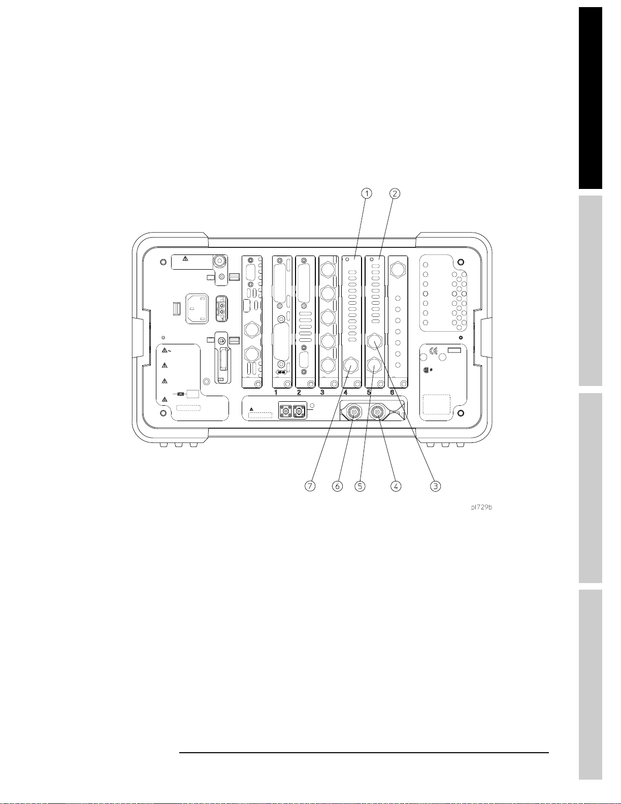
Figure 3-2 Rear-Panel Feature Overview
Getting Started
Instrument Overview
Measurements
Chapter 3 39
Page 40

Getting Started
G
t
tngS
t
ted
AnalysisM
d
M
t
Instrument Overview
ar
e
e
o
Ta bl e 3- 2 K e y t o Figure 3-2 Rear-Panel Feature Overview (above)
1 DSP and Fast
ADC
2RFComms
Hardware
3ExtRefIn Accepts an external 1 MHz to 30 MHz reference frequency source.
410MHzREFIN Accepts an external frequency source to provide the 10 MHz, −15 to +10 dBm
5 10 MHz Out Provides a 10 MHz, 0 dBm minimum, timebase reference signal phase locked to the
610MHzREF
OUT
7 Ext Frame Sync Acceptsanexternal0to5VTTLtrigger.
DSP and Fast ADC (Option B7D) provides digital signal processing and fast ADC
required for many of the digital demodulation measurements in the Modulation
Analysis and other measurement personalities. It must be ordered with Option B7E
andOption1D5.
RF Communications Hardware (Option B7E) provides the RF down convertor
hardware required for digital demodulation measurements. It must be ordered with
Option B7D and Option 1D5.
frequency reference used by the analyzer.
Ext Ref In.
Provides a 10 MHz, 0 dBm minimum, timebase reference signal.
s
easuremen
40 Chapter 3
Page 41

Getting Started
A
n
a
l
y
s
s
M
o
d
e
Options Required
Options Required
Installing the Modulation Analysis measurement personality firmware and making
the associated measurements require certain basic equipment. This section lists
Modulation Analysis compatible Agilent ESA Spectrum Analyzers and required
hardware options.
Compatible Spectrum Analyzers
The Modulation Analysis measurement personality is not compatible with all ESA
spectrum analyzer models. Table 3-3 lists the models that are compatible and the
upper frequency range of each.
Table 3-3 Modulation Analysis Compatible Agilent ESA Spectrum Analyzers
Model Number Upper Frequency Range
E4402B 3 GHz
E4404B 6.7 GHz
E4405B 13.2 GHz
E4407B 26.5 GHz
Hardware Options Required
Additional hardware options must be installed in the spectrum analyzer before
Modulation Analysis measurements can be made. Table 3-4 lists the hardware
options required for optimum performance of Modulation Analysis measurements.
Not all of the options can be installed by the user. Some of the options require that
the instrument be returned to the factory or an Agilent Technologies service center.
In addition, some of the options require Performance Verification and Adjustments
to be performed after installation. Refer to Table 3-4 for option specific
information.
NOTE When transporting the instrument, use the original packaging or comparable
packaging. If the shipping container is damaged, any part is missing, or you do not
have an appropriate shipping container, notify Agilent Technologies at one of the
addresses shown on “Getting in touch with Agilent Technologies, Inc.” on page
182.
Measurements
Chapter 3 41
Page 42

Getting Started
G
t
tngS
t
ted
AnalysisM
d
M
t
Options Required
ar
e
e
o
Table 3-4 Modulation Analysis Hardware Options and Measurements
Required/recommended
option
Modulation Analysis Personality 229 Required for all measurements.
Memory extension B72
DSP and Fast ADC
RF Communications Hardware
High Stability Frequency Reference
RF and Digital Communication
Hardware Option bundle
Option
Number
a
B7D
a
B7E
b
1D5
Option B74
Includes the
following options:
1D6
B72
1D5
B7D
B7E
1DS
1DR
b
Comments
Required
Recommended
Includes necessary hardware for the modulation
analysis measurements personality.
a. Service center or factory installation; calibration required.
b. Factory installation only.
NOTE If the appropriate hardware is not present, the measurement softkey under the
s
Measure menu will be grayed out and that measurement will not be available.
easuremen
42 Chapter 3
Page 43

Getting Started
A
n
a
l
y
s
s
M
o
d
e
Installing Optional Measurement Personalities
Installing Optional Measurement Personalities
Active License Key
The measurement personality software you have purchased with your instrument
has been installed and the license key has been enabled at the factory. With any
future purchase of a new personality software, you will receive a certificate that
displays the unique license key number. The license key enables you to install, or
reinstall, any measurement personality you have purchased. If you return the
instrument to the factory for the installation of measurement personality software,
you will receive no documentation of the license key number, nor will you receive
documentation of the license key number for the measurement personality
software you have purchased with your instrument.
Installing the Licensing Key
If you are installing a new option, follow these steps to install the unique license
key number for the measurement personality software that you want to install in
your instrument:
1. Press
2. Use the alpha editor to enter the three letter designation for the software option
3. Press
4. Press
5. Use the alpha editor to enter the 12 character licensing key number for the
6. Press
7. Press
System, More, Licensing, Option.
When you press
using the alpha editor, refer to the Agilent ESA Spectrum Analyzers User’s
Guide.
that you wish to install in the instrument.
Done on the alpha editor menu.
License Key.
When you press
instructions on using the alpha editor, refer to the Agilent ESA Spectrum
Analyzers User’s Guide.
software option that you wish to install in the instrument.
Done on the alpha editor menu.
Activate to turn on the licensing key. You may now install the
measurement personality option software.
Option the alpha editor will be activated. For instructions on
Licensing Key the alpha editor will be activated. For
Measurements
Chapter 3 43
Page 44

Getting Started
G
t
tngS
t
ted
AnalysisM
d
M
t
Installing Optional Measurement Personalities
ar
e
e
o
s
Using the Install Key
You may want to install a software revision, install new measurement software or
reinstall measurement software that you have previously uninstalled, or uninstall
measurement software. Before you can install software, you will need a set of
installation diskettes.
If you have ordered a measurement personality, you will receive the installation
disk set in the option upgrade package. If you are updating an existing, previously
installed measurement option, you may order the diskettes from Agilent
Technologies or create a set from the Agilent internet site shown in “Updating the
Firmware” on page 48. When you order the updated software disk set, you will
need to order Option UE2. (Option UE2 is a firmware update and is needed to
ensure that the firmware and the software are compatible.) A set of diskettes can be
ordered from your local Agilent Technologies service or sales office. Refer to
“Getting in touch with Agilent Technologies, Inc.” on page 182 for the location of
these offices. To create a disk set refer to “Creating Software Installation Disks”
below.
Creating Software Installation Disks
To create the installation disks on-line, visit the Agilent internet site shown in
“Updating the Firmware” on page 48. Follow the instructions provided on the
internet site for downloading the current measurement personalty software and
creating the installation disk set. The instructions for creating the disk set will step
you through the process to create a firmware disk set when you create the
measurement personalty software disk set. (A firmware update may be needed to
ensure that the firmware and the software are compatible.) After you have created
the disk set, follow the on-line instructions to install the firmware. After
successfully installing the firmware update, proceed with the following
instructions for installing the measurement personalty software in your instrument.
Installing Personality/Software Options
easuremen
NOTE When the installer starts up, it examines the instrument to ensure that all the
This procedure gives steps to install a new software option in an ESA-E Series
Spectrum Analyzer using the internal floppy drive of the instrument. Screen
messages display the update progress and give directions. The instrument will not
need to be re-calibrated after this procedure since no changes are made to
calibration or adjustment files.
If you have a problem with the installation process, refer to “Troubleshooting the
Installer” on page 46.
required software and hardware options are present. If they are not, the installer
will generate an error and you will not be able to install the personality.
1. If this is the installation of new personality option software, you must enter the
License Key for the new option. For instructions on entering the License Key,
refer to the “Installing the Licensing Key” on page 43.
44 Chapter 3
Page 45

Getting Started
A
n
a
l
y
s
s
M
o
d
e
Installing Optional Measurement Personalities
When you have completed entering the license key number, continue with the
next step.
2. Insert disk one of the installation disk set into the disk drive located on the right
side of the ESA front panel.
3. Press
4. When the installer first starts up, it will show a popup message. Select
NOTE Once the installer has begun installing a personality, any error will cause the whole
personality (including a previously installed version) to be removed from the
instrument. Because of this, it is very important that you verify the disks prior to
installing them. If any of the disks or files are bad, you will not be able to use the
personality until you obtain a new installation disk set and run the install using
them.
5. When prompted, insert the next disk and press
6. When the verification is complete, press
System, More, Personalities,andInstall. The instrument will then load
the installer from the floppy drive. If there is no floppy in the drive, the
incorrect disk is inserted, or there is no installer on the disk, the error “No
install disk present in disk drive” will be shown.
Once the instrument has loaded the installer, the screen will change to the
installer screen and the
information on the installer screen and menu, refer to “Installer Screen and
Menu” on page 47.
.
Disks
When Verify Disks is running, the
grayed out.
personality will begin. Some of the disks may take only a short time to load or
be skipped entirely, while others can take up to about 30 minutes to load.
Install Pers. menu will be shown. For more
Verify
Ver ify Disks again.
Install Now and Exit Install keys will be
Install Now and the installation of the
Measurements
When installer is running, the
out.
7. When prompted, insert the next disk and press
8. Once the installation is complete, press
Chapter 3 45
Verify Disk s and Exit Install keys will be grayed
Install Now again.
Exit Install.
Page 46

Getting Started
G
t
tngS
t
ted
AnalysisM
d
M
t
Installing Optional Measurement Personalities
ar
e
e
o
Troubleshooting the Installer
If the installation process stalls or fails in another way, follow these steps to
resolve your problem.
1. If the instrument stops the update process before all the disks are loaded
proceed as follows:
a. Press
b. Return to step 2 under “Installing Personality/Software Options” and start
2. If the instrument fails after repeating the installation procedure, get in touch
with your nearest Agilent sales and service office listed in “Getting in touch
with Agilent Technologies, Inc.” on page 182 for assistance. Please provide
the following information:
Model Number:
Serial Number:
State that you are having trouble installing a software option update.
Exit Install to abort the process.
the installation process again.
s
easuremen
46 Chapter 3
Page 47

Getting Started
A
n
a
l
y
s
s
M
o
d
e
Installing Optional Measurement Personalities
Installer Screen and Menu
The top portion of the install screen is a table in which the files that are about to be
installed are listed. The bottom portion of the screen contains information needed
to track the progress of the install.
Table 3-5 Key to Installer Screen and Menu Screen (above)
1 File Table displays the files to be installed and various file information. If there
aremorethensixfiles,
view additional items.
2FileNamedisplays the name of the files on the installation disk.
3 Current Version displays the version of the file that is currently installed in the
instrument. (This field will be blank if this file is not currently installed in the
instrument or if the file is a data file that has no version.)
4 Upgrade Version shows the version of the file on the install disk. This is the
version of the file that will replace the currently installed version.
5 Status is updated to reflect what the installer is doing to the current file as the
install progress. The valid messages seen in this column are listed in Table 3-6 on
page 48.
6 Data Field contains a status bar and various status information.
7 Processing disk shows the disk that is currently being read.
8 Processing item shows the file that is being processes by item number.
9 Bytes free on C is the number of bytes currently free on the instrument C: drive.
10 Status Bar contains a status bar that runs from 0 to 100% and tracks the progress
of the current step and a message line displays the step that is currently being
executed.
Next Item and Prev Item allow you to scroll the table to
Measurements
Chapter 3 47
Page 48

Getting Started
G
t
tngS
t
ted
AnalysisM
d
M
t
Installing Optional Measurement Personalities
ar
e
e
o
Table 3-5 Key to Installer Screen and Menu Screen (above)
11 B y tes i n package lists the number of bytes in the install package/ fill.
12 Bytes left in package lists the number of bytes left to be read.
13 Message and error popup window that displays over the status bar. Information in
this box will prompt you for action required to proceed to the next phase of the
installation. It may also inform you of errors in the installation process and may
prompt you for action required to correct the problem.
Table 3-6 Installer Status Messages
Failed This means that something has gone wrong while processing this item. It
is a fatal error and the installation can not be completed. The installer
will try to get the system back to a good state which may entail
completely removing the currently installed personality.
Loading The file is currently being copied from the install media to the
instrument’s file system.
Verifying This may mean one of two things:
1. If “Verify Disks” was pressed then Verifying means that the installer
is currently reading the install media and comparing the known
checksums to ensure the data is good.
2. If “Install Now” was pressed, then Verifying means that the installer
is reading what was just loaded to ensure the checksum is correct.
Loaded This means that the data has been placed on the instrument disk but has
s
Installed This means that the data has been loaded into the instrument and
easuremen
Skipping This means that the installer has determined that this file does not need
not yet been registered with the firmware.
registered. The install for this file is complete.
to be loaded into the instrument.
Agilent ESA Spectrum Analyzers Update
For the latest information about this instrument, including firmware upgrades,
application information, and product information, please visit the URL listed
below.
Updating the Firmware
Updated versions of the ESA-E Series Spectrum Analyzer firmware will be
available via several sources. Information on the latest firmware revision can be
accessed from the following URL:
http://www.agilent.com/find/esa/
48 Chapter 3
Page 49

A
n
a
l
y
s
s
M
o
d
e
M
t
4 Setting Up the Modulation Analysis
Mode
This chapter introduces you to the basic measurement process.
easuremen
s
49
Page 50

G
t
tngS
t
ar
ted
AnalysisM
d
M
t
Setting Up the Modulation Analysis Mode
Preparing to Make Measurements
e
Preparing to Make Measurements
At initial power up, the analyzer will be in spectrum analyzer (SA) mode and the
FREQUENCY Channel menu displayed. To access the Modulation Analysis
measurement personality, press the
Analysis
key.
Initial Settings
If you have already been into Modulation Analysis mode since the instrument was
powered up and you have not performed a preset, then the screen displayed and the
e
o
settings in force will be exactly as they were when you last switched out of
Modulation Analysis mode.
When you put the instrument into Modulation Analysis mode for the first time
after a power up, the Monitor Spectrum screen will be displayed with a center
frequency setting of 1.0 GHz and a span of 6 MHz. This Monitor Spectrum
function allows you to check that there is a signal to be measured.
The center frequency can be changed by pressing
required frequency using the numeric keys. The span can be altered by pressing
Span and entering the required span using the numeric keys.
Before making a measurement, make sure the mode setup and radio standard
parameters are set to the desired settings. Refer to Chapter 6 , “Menu Maps,” and
Chapter 7 , “Front Panel Key Reference,” for additional information to guide you
in changing parameter settings.
MODE key and select the Modulation
Frequency andthenenteringthe
s
easuremen
You can set the instrument to use
under the System front panel key. If you set the preset to Mode or to Factory,
pressing Preset causes the analyzer to immediately reset all parameters to that
particular setting. Note that a Factory Preset will switch modes, returning the
ESA to the Spectrum Analysis mode. You will then have to re-access the
Modulation Analysis mode after the preset operation is completed.
If you set the preset to User, the instrument displays a Preset menu when you
Preset.ThePreset menu allows you to select the User defaults, Mode
press
defaults or the Factory defaults. For more information on setting, saving, and
using user defaults, refer to the ESA Spectrum Analyzers User’s Guide.
If you want to set only the Modulation Analysis mode to a known, factory default
state, press Mode Setup and Restore Mode Setup Defaults. This will reset only
the Mode parameters to the factory defaults without affecting the SA mode, and
the instrument will not exit the Modulation Analysis mode.
To preset only the settings that are specific to the selected measurement, press
Restore Meas Defaults under Meas Setup. This will set the measurement setup
parameters, for the currently selected measurement only, to the factory defaults.
User preset, Mode preset or Factory preset
50 Chapter 4
Page 51

Setting Up the Modulation Analysis Mode
A
n
a
l
y
s
s
M
o
d
e
Preparing to Make Measurements
How to Make an EVM (Error Vector Magnitude) Measurement
The EVM (Error Vector Magnitude) measurement is set up and is intended to be
used as a “one-button” measurement. After you have properly connected the
instrument to the digital communications system equipment and selected the EVM
measurement, the measurement is made using the default parameters defined by
the selected standard.
You may change the default settings using
Meas Setup key. However, changing
the default settings may produce measurement results that are outside of the
parameters of the selected standard.
Most measurements can be performed using the simple four-step procedure
outlined in the table below using the keys shown in the figure. Most measurements
are performed using only the primary keys listed in conjunction with a minimum
of setup keys. Measurement setup keys (
Meas Setup) can be used for
non-standards compliant testing. For more information see “Initial Settings”.
Step Primary Key Setup Keys Related Keys
1. Select and setup mode
2. Select and setup measurement MEASURE Meas Setup,
3. Select and setup view View/Trace Span X Scale,
4. Saving and printing results File
MODE Mode Setup System
Meas Control,
Print
Restore Meas Defaults,
FREQUENCY Channel
Amplitude Y Scale
Print Setup Save
, Display
Restart
Marker
, Search
Measurements
Chapter 4 51
Page 52

Setting Up the Modulation Analysis Mode
G
t
tngS
t
ted
AnalysisM
d
M
t
Preparing to Make Measurements
ar
e
e
o
How to Save Measurement Results
To save measurement results follow the process shown below. For additional
information on file management in the spectrum analyzer, refer to the ESA
Spectrum Analyzers User’s Guide.
1. Press
2. If you want to change the file name, press
3. The default directory is the C: drive. If you want to change the file directory,
4. Press
5. If you have used the default file name and wish to save additional measurement
6. If you have not used the default file name and wish to save additional
File, Save, Type, More, Measurement Results.
Name, and use the Alpha Editor to
enter the new name. For more information on using the Alpha Editor, refer to
the ESA Spectrum Analyzers User’s Guide.
Dir Up (or Dir Select
press
directory and then press Dir Select.
Save Now to complete the file saving process.
results, press
default file name.
measurement results, repeat steps 1 through 3.
Save. The current measurement result will be saved with the next
)
and use the up or down arrows to select the desired
s
easuremen
52 Chapter 4
Page 53

A
n
a
l
y
s
s
M
o
d
e
M
t
5 Making Modulation Analysis
Measurements
This chapter shows how to make modulation analysis measurements and how to
interpret them. Various radio signals having different problems are shown and
compared against results of acceptable signals.
easuremen
s
53
Page 54

G
t
tngS
t
ar
ted
AnalysisM
d
M
t
Making Modulation Analysis Measurements
What You Will Find in This Chapter
e
What You Will Find in This Chapter
The Modulation Analysis Personality Page 5-55
Purpose Page 5-55
Measurement Method for a CDMA System Page 5-56
Making a CDMA Measurement Page 5-57
Interpreting Measurement Results Page 5-64
Baseband Filtering Errors Page 5-64
e
o
I/Q Gain Imbalance Page 5-69
I/Q Quadrature (Skew) Error Page 5-71
Symbol Rate Error Page 5-74
I/Q DC Offset Error Page 5-77
In-Channel Phase Modulation Interference Page 5-78
In-Channel Amplitude Modulation Interference Page 5-81
In-Channel Spurious Signal Interference Page 5-85
Measuring a Custom QPSK Format Signal Page 5-87
Other Customized Changes You Can Make Page 5-88
Problems Obtaining a Measurement Page 5-89
s
easuremen
54 Chapter 5
Page 55

Making Modulation Analysis Measurements
A
n
a
l
y
s
s
M
o
d
e
The Modulation Analysis Personality
The Modulation Analysis Personality
Purpose
A thorough analysis of EVM (error vector magnitude) in a digital communication
system is invaluable for troubleshooting common errors such as:
I/Q error
Symbol rate errors
Wrong filter coefficients
Wrong interpolation, IF filter tilt, or ripple
LO instability
Tone interference
AM/PM conversion errors
The Agilent Modulation Analysis Measurement Personality provides this analysis
of digitally-modulated signals for the following major cellular standards:
W-CDMA (3GPP)
cdmaOne (IS-95 and J-STD-008)
cdma2000 SR1
NADC
GSM
EDGE
PDC
TETRA
In addition, the personality allows you to alter the filters and symbol rates defined
by the communication standards if the signal you are analyzing differs from a
defined radio standard.
This guide shows you how to set up the Agilent ESA to measure and display the
results of EVM using eye, constellation, and vector diagrams (when measuring
appropriate radio standards), as well as tabular data. The key results provided are:
Peak and RMS EVM
Peak and RMS Magnitude error
Peak and RMS Phase error
Frequency error
I/Q offset
Droop error
EVM versus symbol display
Magnitude error versus symbol display
Phase error versus symbol display
Polar vector display
Polar constellation display
I and Q eye display
Measurements
Chapter 5 55
Page 56

Making Modulation Analysis Measurements
G
t
tngS
t
ted
AnalysisM
d
M
t
The Modulation Analysis Personality
ar
e
e
o
Measurement Method for a CDMA System
Consider making an EVM measurement on a CDMA system.
You can only make an EVM measurement intrusively. When you perform the
measurement, a carrier channel with a single pilot channel are the only allowed
active channels. No other traffic channels or paging channels may be present.
The intrusive method takes the measurement directly from the RF output port of
the transceiver, as shown in Figure 5-1.
CAUTION If you take the measurement directly from the RF output port of the transceiver,
ensure that the power level at the RF input of the spectrum analyzer does not
exceed the damage level of 30 dBm.
Because you disconnect the antenna from the transceiver and disrupt the
transmission signal, this cannot be considered a non-intrusive test. The transceiver
will not be able to communicate with users on the system.
You may also make a less intrusive test by connecting a directional coupler to the
RF output with the main arm connected to the antenna and the coupled port
connected to the spectrum analyzer, as shown in Figure 5-2.Youmustensurethat
only the pilot Walsh channel is active. Because only a pilot channel will be
observed, the transceiver will not be able to communicate with users on the
system.
NOTE The timebase of the base station and the spectrum analyzer should be locked
together. These are referred to as “10 MHz Ref In” or “Ext Ref In” throughout the
remainder of this document.
s
easuremen
56 Chapter 5
Page 57

Making Modulation Analysis Measurements
A
n
a
l
y
s
s
M
o
d
e
Making a Wideband CDMA Measurement
Making a Wideband CDMA Measurement
NOTE Use the Help key to get a quick explanation of any Modulation Analysis
Personality key, as well as any equivalent SCPI command that performs the
function of that key.
1. Install the Modulation Analysis Measurements Personality as described in the
“Getting Started” chapter of this guide.
2. Make sure that the base transceiver station is in service with only the pilot
Walsh channel active.
3. Connect the device being measured and the spectrum analyzer input as shown
in Figure 5-1 or Figure 5-2.
Figure 5-1 Measurement Setup
Measurements
Chapter 5 57
Page 58
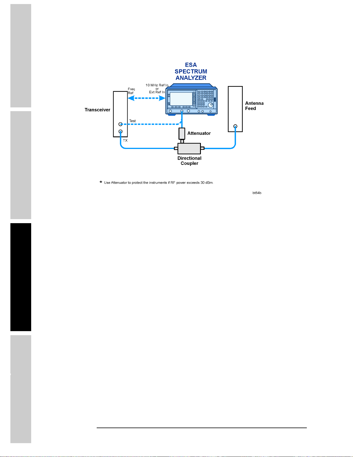
Making Modulation Analysis Measurements
G
t
tngS
t
ted
AnalysisM
d
M
t
Making a Wideband CDMA Measurement
ar
e
e
o
Figure 5-2 Alternative Measurement Setup
4. Press Mode, Modulation Analysis, Mode Setup, Radio Std and choose the
radio standard being used.
5. Press
6. Press
s
FREQUENCY and set the center frequency to the transmit frequency of
the radio.
MEASURE, Monitor Spectrum and check to see that the spectrum looks
reasonable. It should be centered on the display with modulation present, as
shown in Figure 5-3 (Wideband CDMA signal shown). If not, then refer to
“Problems Obtaining a Measurement” later in this chapter.
easuremen
58 Chapter 5
Page 59
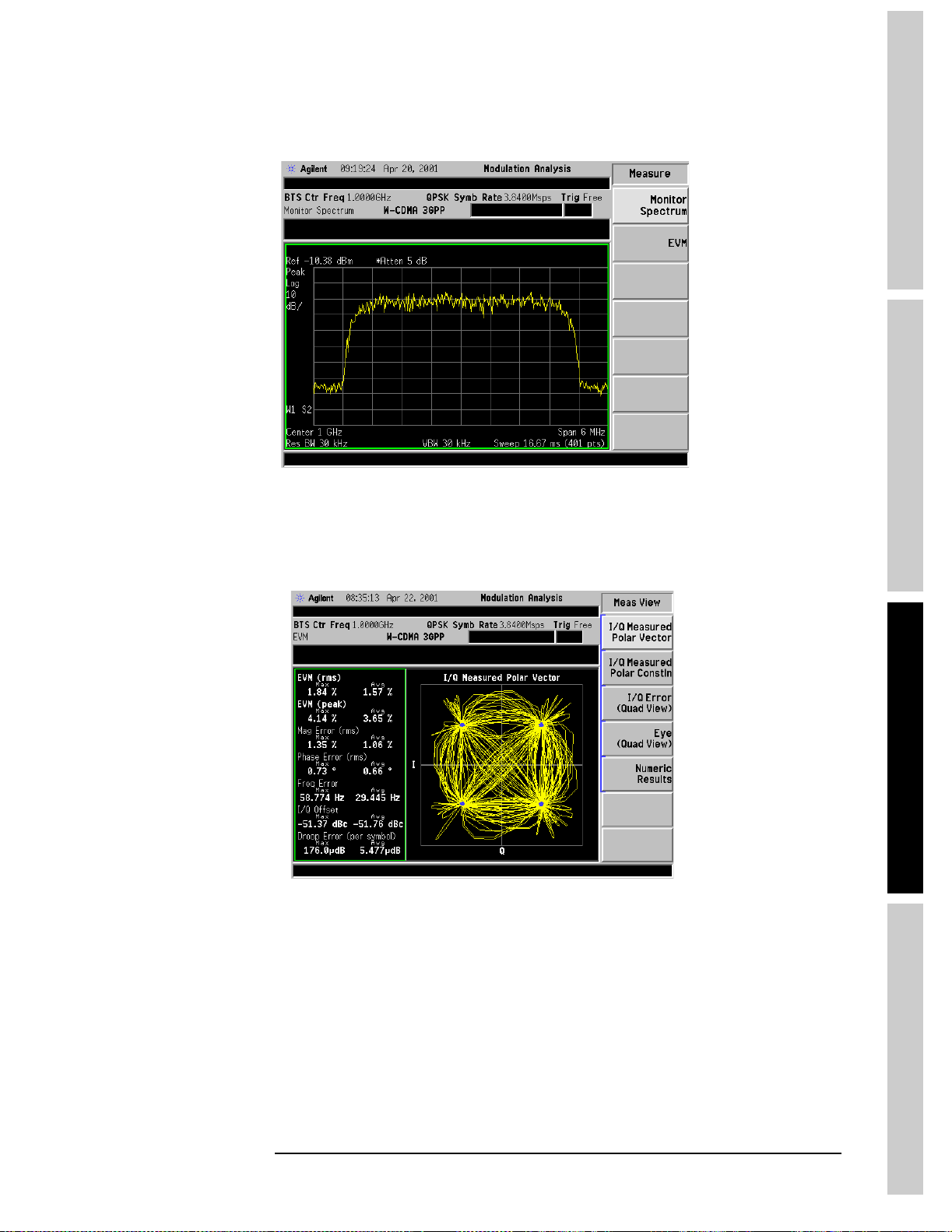
A
n
a
l
y
s
s
M
o
d
e
Figure 5-3 Monitor Spectrum Display
Making Modulation Analysis Measurements
Making a Wideband CDMA Measurement
7. Press
Figure 5-4 Polar Vector Display
8. Press
EVM. You should see an I/Q polar vector display of the signal, similar to
that shown in Figure 5-4. Results are listed in a table left of the vector display.
View/Trace, I/Q Measured Polar Constln. You should see an I/Q polar
constellation display of the signal and the table of critical parameter values,
similar to that shown in Figure 5-5.
Measurements
Chapter 5 59
Page 60

G
t
tngS
t
ar
ted
AnalysisM
d
M
t
e
Making Modulation Analysis Measurements
Making a Wideband CDMA Measurement
NOTE As a troubleshooting tool, you can manually build the polar constellation or step
through the trace with a short line segment using the I/Q Points and I/Q Points
Offset
keys.
Whenyoumakeasinglemeasurement(pressthe
the data for that single measurement is held within instrument memory. If you then
set the
slowly increasing the I/Q Points figure from zero using the RPG knob.
Similarly you can set the
the I/Q Points Offset figure using the RPG knob. Now you will see a ‘snake’
marking out the signal’s trace on the display.
I/Q Points Offset to 0, you can see how the measurement is built up by
I/Q Points figure to a low number (say, 5 or 10) and vary
Single key on the front panel),
e
o
Figure 5-5 Polar Constellation Display
s
9. Press
easuremen
I/Q Error (Quad View) and refer to Figure 5-6. You should see graphical
displays of magnitude error versus time, phase error versus time, EVM versus
time, and tabular results.
60 Chapter 5
Page 61

Making Modulation Analysis Measurements
A
n
a
l
y
s
s
M
o
d
e
Making a Wideband CDMA Measurement
Figure 5-6 I/Q Errors Showing Magnitude, Phase, and EVM
10. Press
11. Press
12. Change the y-axis scaling (% for EVM, Magnitude, and ° for Phase Error
13. The blue data points shown along the traces are the symbol decision point
Next Window (a key located below the display). Each of the four
individual windows are “highlighted” by a colored border as you press this key.
Press
Next Window again and then press Zoom. The size of the selected
window expands for easier viewing.
Next Window to select one of the time graphs and then press Zoom.
Change the x-axis scaling (number of symbols) to 2/division by pressing
SPAN, Scale/Div, 2, Sym. This menu also allows you to change the x-axis
reference value and position.
graphs) to 0.5/division by pressing
menu also allows you to change the y-axis reference value and position.
locations. To turn these off, press
menu also allows you to change I/Q points and points/symbol. Press
return to normal viewing.
AMPLITUDE, Scale/Div, .5, % (or °.) This
Display, Symbol Dots Quad View, Off.This
Zoom to
Measurements
Chapter 5 61
Page 62
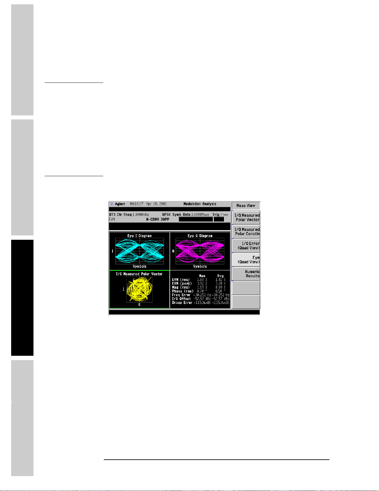
G
t
tngS
t
ar
ted
AnalysisM
d
M
t
e
Making Modulation Analysis Measurements
Making a Wideband CDMA Measurement
14.Press View/Trace, Eye (Quad View) and refer to Figure 5-7. You should see
individual eye diagrams for I and Q, along with a polar vector display, and
tabular results of critical parameter values.
NOTE As a troubleshooting tool, you can manually build the polar constellation or step
through the trace with a short line segment using the
Offset
keys.
I/Q Points and I/Q Points
Whenyoumakeasinglemeasurement(pressthe
the data for that single measurement is held within instrument memory. If you then
set the I/Q Points Offset to 0, you can see how the measurement is built up by
slowly increasing the
e
o
Figure 5-7 Eye Diagrams with Polar Vector Constellation
Similarly you can set the
the
I/Q Points Offset figure using the RPG knob. Now you will see a ‘snake’
marking out the signal’s trace on the display.
I/Q Points figure from zero using the RPG knob.
I/Q Points figure to a low number (say, 5 or 10) and vary
Single key on the front panel),
s
easuremen
62 Chapter 5
Page 63
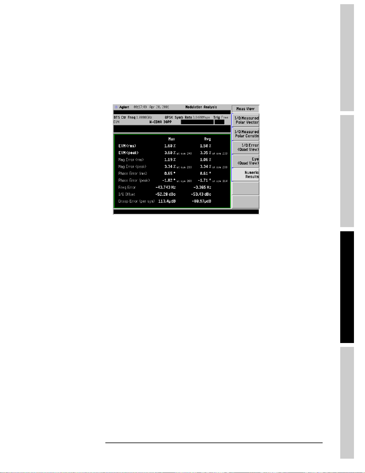
A
n
a
l
y
s
s
M
o
d
e
15. Press Numeric Results and refer to Figure 5-8. You should see a tabular
display of the critical parameter values similar to the tables in the previous
views. This table differs in that it also includes peak values for magnitude error
and phase error. The specific symbols are identified with each of these values.
Figure 5-8 Numeric Results View
Making Modulation Analysis Measurements
Making a Wideband CDMA Measurement
Measurements
Chapter 5 63
Page 64
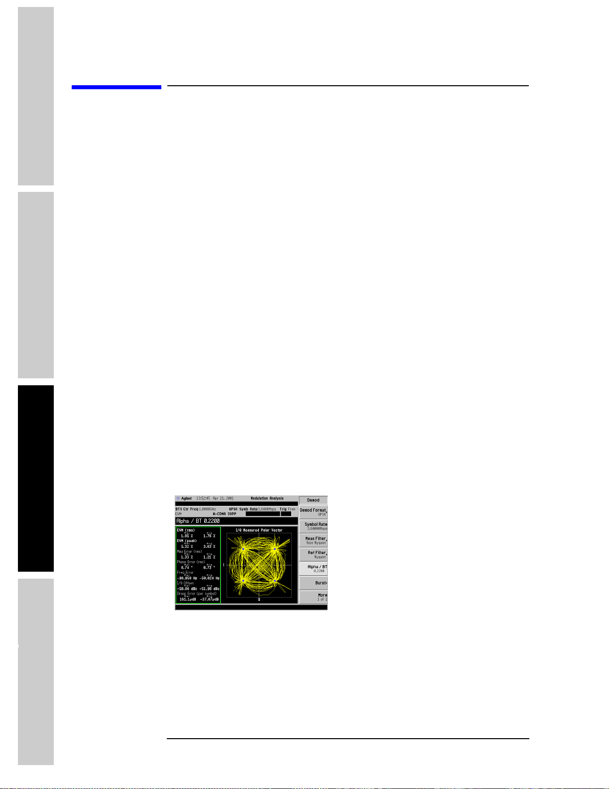
G
t
tngS
t
ar
ted
AnalysisM
d
M
t
Making Modulation Analysis Measurements
Interpreting Measurement Results
e
Interpreting Measurement Results
The power of the Modulation Analysis Personality is its ability to characterize the
radio signal for transmitter troubleshooting. This section illustrates how to
interpret the data to indicate symptoms of problems in radio signals.
The following radio signal errors are investigated in this section:
Baseband Filtering Errors
I/Q Gain Imbalance
I/Q Quadrature (Skew) Error
I/Q DC Offset Error
e
o
Symbol Rate Error
I/Q DC Offset Error
In-Channel Phase Modulation Interference
In-Channel Amplitude Modulation Interference
In-Channel Spurious Signal Interference
Baseband Filtering Errors
Filtering errors are among the most common in digital communication design.
Typical filter errors can be due to errors in filter alpha, wrong filter shape, or
incorrect filter coefficients. The result is increased intersymbol interference.
Lower peak overshoot is also caused by signal compression, which can indicate
that an amplifier stage is being overdriven.
1. The vector diagram gives the first indication of baseband filtering errors. Press
I/Q Measured Polar Vector. The display should look similar to that shown in
s
Figure 5-9 Polar Vector of Signal Using a 0.22 Filter α
Figure 5-9. This is a normal Wideband CDMA signal shown with a filter α of
0.22.
easuremen
64 Chapter 5
Page 65

Making Modulation Analysis Measurements
A
n
a
l
y
s
s
M
o
d
e
Interpreting Measurement Results
2. In contrast, refer to Figure 5-10. A Wideband CDMA signal is shown with a
filter α of 1. Observe that there are smaller overshoots in the trajectories
between the symbol points (item 1) due to the increased alpha. This limits the
required peak power and reduces the transmitter power requirements. Item 2
shows spreading of the decision points due to the increased EVM (item 3.)
NOTE To change the filter α of the analyzer, press Det/Demod, Alpha/BT.
Figure 5-10 Polar Vector of Signal Using a 1.0 Filter α
Measurements
Chapter 5 65
Page 66
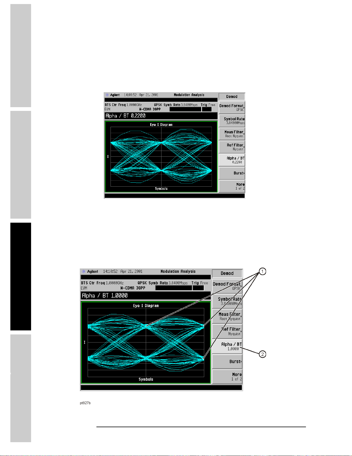
G
t
tngS
t
ar
ted
AnalysisM
d
M
t
e
e
o
Making Modulation Analysis Measurements
Interpreting Measurement Results
3. Press View/Trace, Eye (Quad View), Next Window, Next Window, Next
Window, Zoom
(W-CDMA signal shown with filter α = 0.22.)
Figure 5-11 I Eye Diagram of Signal Using a 0.22 Filter α
. The display should look similar to that shown in Figure 5-11
4. In contrast, refer to Figure 5-12. This shows a Wideband CDMA signal with a
filter α of 1 (item 2). An incorrect filter alpha is indicated when the center
diamond shape is distorted with rounding and widened crossover points at the
top and bottom corners (item 1.) The eye diagram tends to “spread out” in this
case.
s
Figure 5-12 I Eye Diagram of Signal Using a 1.0 Filter α
easuremen
66 Chapter 5
Page 67
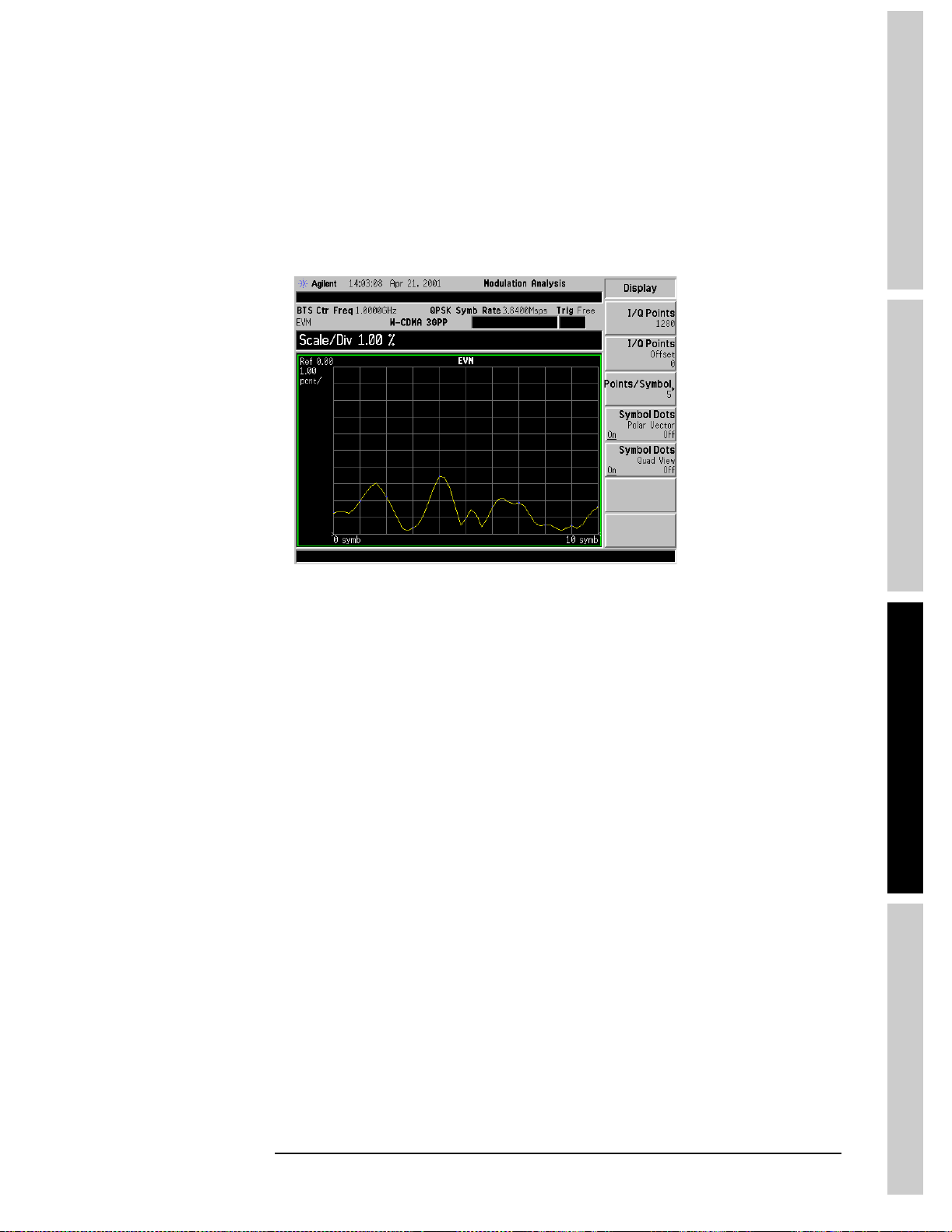
Making Modulation Analysis Measurements
A
n
a
l
y
s
s
M
o
d
e
Interpreting Measurement Results
5. Press View/Trace, I/Q Error (Quad View).PressNext Window until the EVM
graph is highlighted. Press Zoom,Amplitude,Scale/Div,6,%to expand the
y-axis scale. Press SPAN, Scale/Div, 1, Sym to expand the x-axis scale. The
result of a “normal” signal is shown in Figure 5-13 (W-CDMA signal shown
with filter α = 0.22.)
Figure 5-13 Zoomed EVM Display of Signal Using a 0.22 Filter α
Measurements
Chapter 5 67
Page 68

G
t
tngS
t
ar
ted
AnalysisM
d
M
t
e
e
o
Making Modulation Analysis Measurements
Interpreting Measurement Results
6. In contrast, refer to Figure 5-14 (W-CDMA signal shown with
filter α=1.)
Differing filter alphas between the transmitter and receiver do not significantly
affect the symbol locations. However, differing alphas do cause incorrect
transitions. As a result, the error vector is large between symbol points and
relatively small at the symbol locations (item 1.)
Figure 5-14 Zoomed EVM Display of Signal Using a 1.0 Filter α
s
easuremen
68 Chapter 5
Page 69

Making Modulation Analysis Measurements
A
n
a
l
y
s
s
M
o
d
e
Interpreting Measurement Results
I/Q Gain Imbalance
I/Q gain imbalance is a result of non-equal gains in the I and Q parts of the
network. This can be caused by differences in components such as filters,
amplifiers, and DACs. For non-scrambled or spread QPSK signals, the symptom
of this imbalance is indicated by rectangular-shaped groupings of symbol decision
points in each quadrant.
Press
Meas Control, Pause to view a single time record.
1. Use the I/Q polar constellation diagram first to identify this problem. Press
View/Trace, I/Q Measured Polar Constln. A signal with an I/Q gain
imbalance is shown in Figure 5-15. A rectangular shape is indicated with the
symbol decision points at the rectangle corners, instead of the square shape you
would normally see with a properly balanced signal. A gain imbalance of 2 dB
was used to obtain this result.
NOTE The long side of the rectangle appears along the I axis, but this will shift 90° along
the Q axis and back again in random fashion. This is normal.
The analyzer arbitrarily assigns the demodulated symbols to the I and Q channels
for each new time record; the analyzer acts as an asynchronous receiver. For this
reason, it is not possible to determine the correct carrier phase reference.
Although the display indicates a Wideband CDMA format, the signal shown is
a non-scrambled or spread QPSK signal.
Figure 5-15 Polar Constellation Showing an I/Q Gain Imbalance
Measurements
Chapter 5 69
Page 70
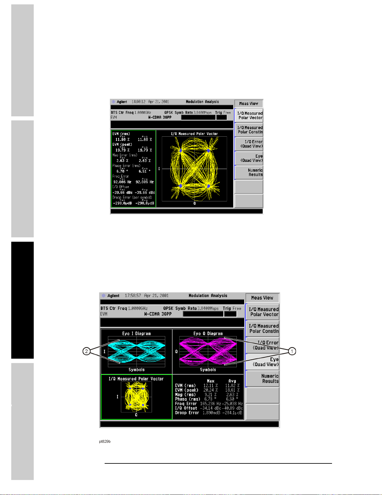
G
t
tngS
t
ar
ted
AnalysisM
d
M
t
e
e
o
Making Modulation Analysis Measurements
Interpreting Measurement Results
2. The polar vector diagram is shown in Figure 5-16. Observe that the rectangular
shape has shifted by 90°, with the longer side of the rectangle along the Q axis.
As stated earlier, this is normal, and will arbitrarily shift back and forth.
Figure 5-16 Polar Vector Showing an I/Q Gain Imbalance
3. Figure 5-17 shows the same signal using the eye diagram. Observe that with a
gain imbalance, the I and Q eye diagrams will not be similar in shape, and these
shapes will be swapped back and forth between each other. In this figure, the Q
eye diagram vertical amplitude (item 1) is greater than that of the I eye diagram
(item 2.)
s
Figure 5-17 Eye Diagram Showing an I/Q Gain Imbalance
easuremen
70 Chapter 5
Page 71

Making Modulation Analysis Measurements
A
n
a
l
y
s
s
M
o
d
e
Interpreting Measurement Results
I/Q Quadrature (Skew) Error
Quadrature error is due to lack of a 90 degree phase shift between the I and Q
channels of a transmitter.
For non-scrambled or spread QPSK signals, the symptom of quadrature error is
indicated by parallelogram-shaped groupings of symbol decision points in each
quadrant.
Press
Meas Control, Pause to view a single time record.
1. Use the I/Q polar constellation diagram first to identify this problem. Press
Measured Polar Constln
Figure 5-18. A parallelogram shape is indicated with the symbol decision
points at the rectangle corners. A quadrature difference of 10° was used to
obtain this result.
Figure 5-18 Polar Constellation Showing I/Q Quadrature Error
. A signal with an I/Q quadrature error is shown in
I/Q
Measurements
NOTE The shape of the parallelogram will shift 90° along the two axes and back again in
random fashion. This is normal.
The analyzer arbitrarily assigns the demodulated symbols to the I and Q channels
for each new time record; the analyzer acts as an asynchronous receiver. For this
reason, it is not possible to determine the correct carrier phase reference.
Although the display indicates a Wideband CDMA format, the signal shown is
a non-scrambled or spread QPSK signal.
Chapter 5 71
Page 72

G
t
tngS
t
ar
ted
AnalysisM
d
M
t
e
e
o
Making Modulation Analysis Measurements
Interpreting Measurement Results
2. The polar vector diagram is shown in Figure 5-19.Observethatthe
parallelogram shape has shifted by 90°. As stated earlier, this is normal, and
will arbitrarily shift back and forth.
Figure 5-19 Polar Vector Showing I/Q Quadrature Error
s
easuremen
72 Chapter 5
Page 73

Making Modulation Analysis Measurements
A
n
a
l
y
s
s
M
o
d
e
Interpreting Measurement Results
3. The zoomed I eye diagram is shown in Figure 5-20. Observe that with a
quadrature error, the crossover points alternately shift between time records.
Because of this, an open triangle pattern begins to take shape at the decision
points (item 1.)
Figure 5-20 Zoomed I Eye Diagram Showing I/Q Quadrature Error
Measurements
Chapter 5 73
Page 74
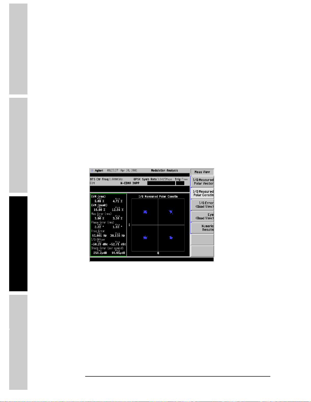
Making Modulation Analysis Measurements
G
t
tngS
t
ted
AnalysisM
d
M
t
Interpreting Measurement Results
ar
e
e
o
Symbol Rate Error
Small deviations in the symbol clock can result in significant modulation errors.
Even a small error in symbol rate causes a large increase in peak EVM, and is
indicated by a spreading of the symbol decision points.
Large symbol rate errors will result in the receiver not being able to demodulate
the signal. The Modulation Analysis Personality is most useful in troubleshooting
small symbol rate errors. To troubleshoot circuits with large symbol rate errors, try
using the ESA occupied bandwidth measurement function to view the signal
channel bandwidth. You can roughly approximate the symbol rate using this
method.
1. Use the I/Q polar constellation diagram first to identify symbol rate errors.
I/Q Measured Polar Constln. A signal with symbol rate errors is shown
Press
in Figure 5-21. Note the spreading of the symbol decision points and large
values of EVM. A symbol rate error of 0.0015 Msps over the actual symbol
rate was used to obtain this result.
Figure 5-21 Polar Constellation Showing Symbol Rate Error
s
easuremen
74 Chapter 5
Page 75
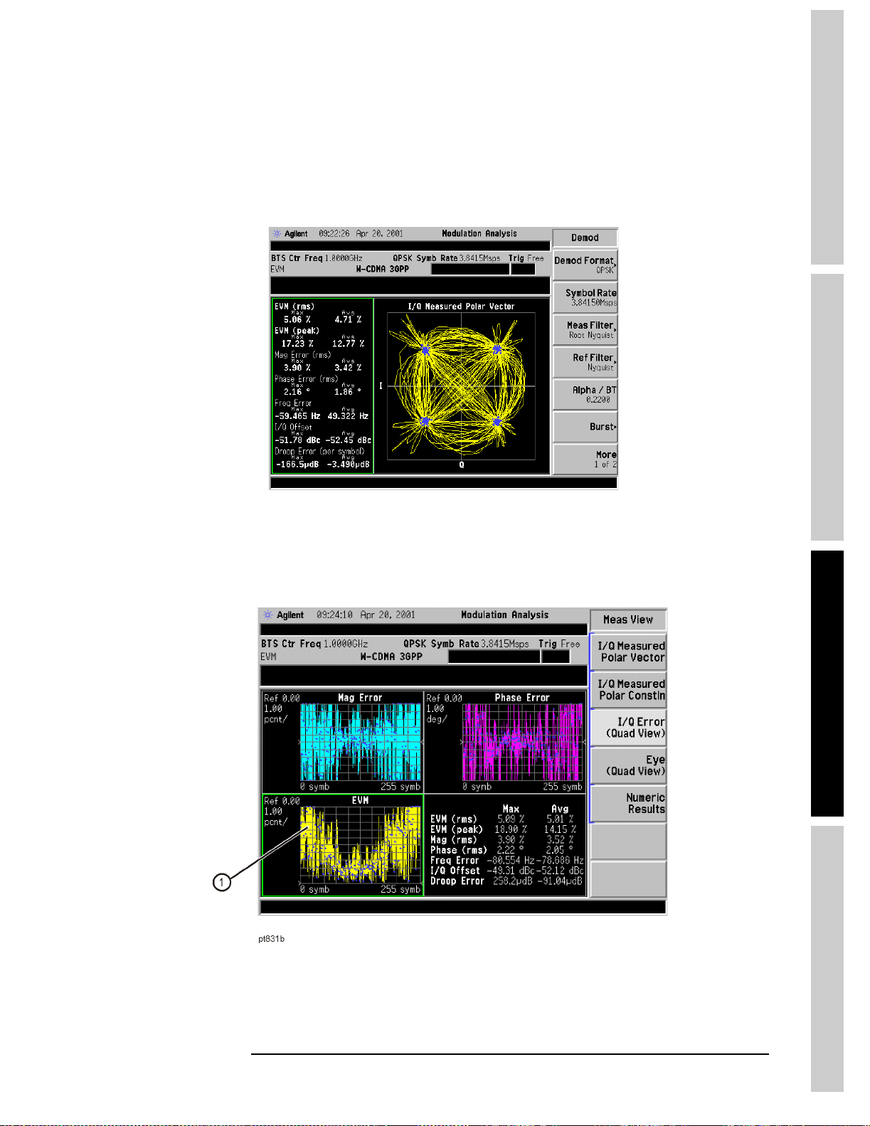
Making Modulation Analysis Measurements
A
n
a
l
y
s
s
M
o
d
e
2. Figure 5-22 shows the polar vector diagram of this signal, with a received
symbol rate of 3.84150 Msps (this symbol rate can be seen above the vector
diagram in the figure.) The transmitted symbol rate is 3.840 Msps.
Figure 5-22 Polar Vector Showing Symbol Rate Error
Interpreting Measurement Results
3. Figure 5-23 shows the I/Q error views of this signal. Observe at item 1 that
with a symbol rate error, the EVM versus time graph shows a “V” shape.
Figure 5-23 I/Q Error Diagram Showing Symbol Rate Error
Measurements
Chapter 5 75
Page 76

G
t
tngS
t
ar
ted
AnalysisM
d
M
t
e
e
o
Making Modulation Analysis Measurements
Interpreting Measurement Results
4. Figure 5-24 shows the EVM versus time graph in zoom mode. The
characteristic “V” shape is caused by the demodulator aligning the expected
symbol clock rate with the clock rate of the signal, for best fit at the midpoint of
the trace. The differences in the two clocks show increasing “slip,” or deviation
further from the trace center. At one arbitrary reference sample, the signal is
sampled correctly. But since the symbol rate is skewed, any other sample in the
positive or negative direction is slightly off in time. This causes an error which
increases linearly in time.
Figure 5-24 Zoomed EVM Versus Symbol Display Showing Symbol Rate Error
s
easuremen
76 Chapter 5
Page 77
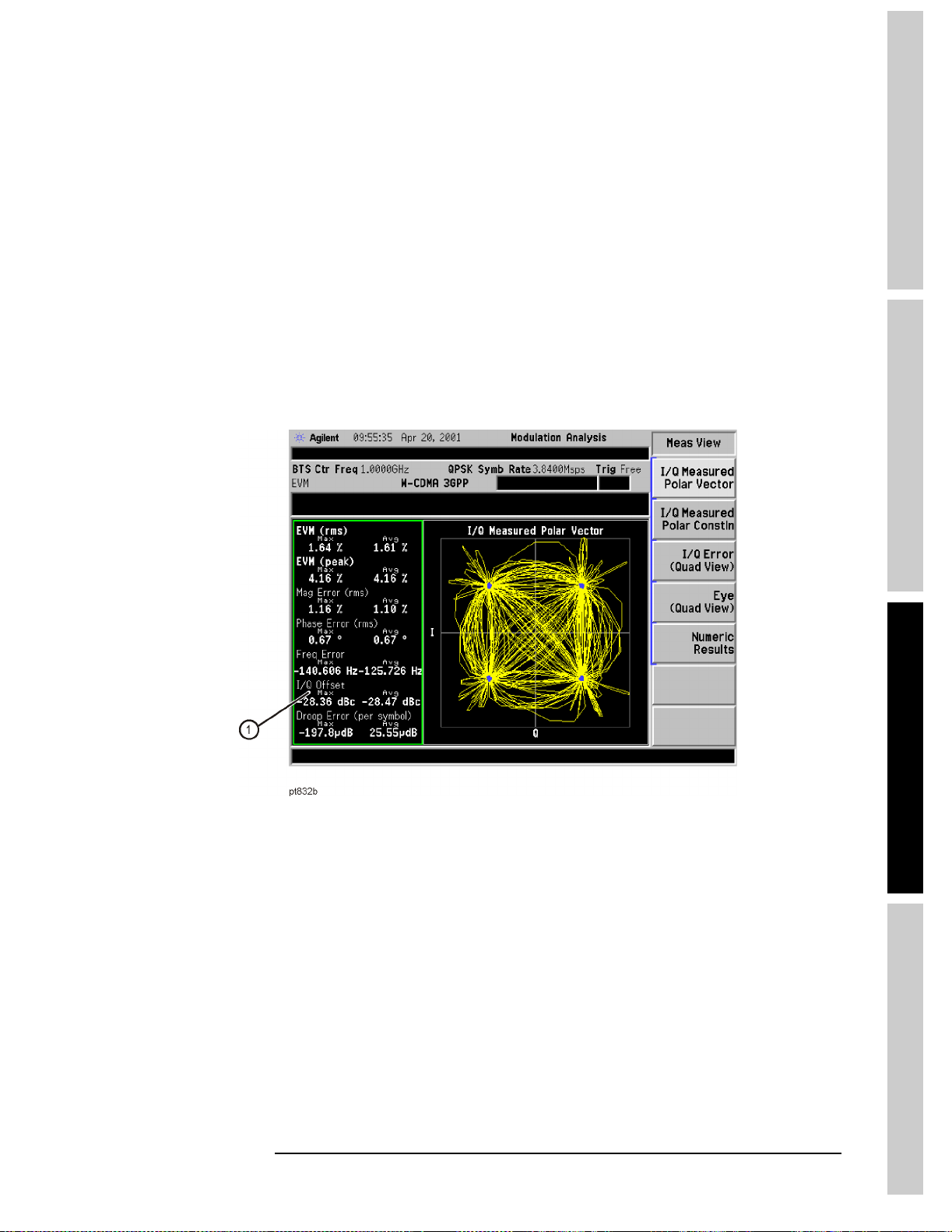
Making Modulation Analysis Measurements
A
n
a
l
y
s
s
M
o
d
e
I/Q DC Offset Error
DC offset is characteristic of an improperly adjusted balanced modulator.
Typically, these offsets are added in the amplifier in the I and Q paths. This type of
error should be indicated in a displaced constellation from the origin of the I/Q
plane. However, any DC offset is reported in the summary/symbol table only, since
the analyzer measures and removes this offset during demodulation.
1. Use the I/Q polar constellation diagram to identify I/Q DC offset errors. Press
I/Q Measured Polar Vector. A signal with an I/Q DC offset error is shown in
Figure 5-25. Observe that there are no noticeable errors shown in the vector
diagram itself. However, the I/Q offset value in the table is about –28 dBc
(item 1), and should be closer to –52 dBc for a Wideband CDMA signal.
Figure 5-25 Polar Vector Showing I/Q DC Offset Error
Interpreting Measurement Results
Measurements
Chapter 5 77
Page 78
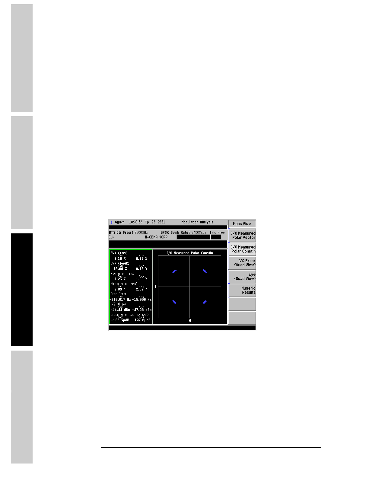
Making Modulation Analysis Measurements
G
t
tngS
t
ted
AnalysisM
d
M
t
Interpreting Measurement Results
ar
e
e
o
In-Channel Phase Modulating Interference
Many signals are present in an integrated communications system. Examples may
include digital, baseband, IF, and RF signals. Crosstalk between adjacent
components and stages often leads to unwanted signals in the output. The
Modulation Analysis Personality can help identify these signals, including
in-channel phase modulating signals.
For a Wideband CDMA signal, PM interference appears as an aligning of the
symbol decision points in the center of each quadrant, forming “lines” of dots. This
line extends farther outward as the magnitude of the PM increases.
1. Use the I/Q polar constellation diagram first to identify this problem. Press
Measured Polar Constln
CDMA signal with in-channel phase modulation interference. Note the
variation of phase around the ideal symbol reference points. Also observe how
much larger the phase error values are compared to those for magnitude error in
the table.
The results shown were created with a phase modulation deviation of 0.03 pi
radians (about 5.5°) and a modulating frequency of 45 kHz.
Figure 5-26 Polar Constellation Showing PM Interference
. Figure 5-26 shows an example of a Wideband
I/Q
s
easuremen
78 Chapter 5
Page 79
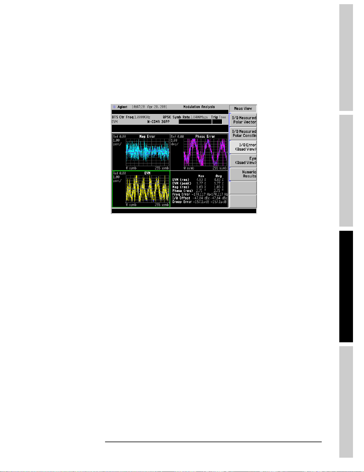
Making Modulation Analysis Measurements
A
n
a
l
y
s
s
M
o
d
e
2. The I/Q error views are shown in Figure 5-27. Observe that the sinusoidal
modulating waveform of the interfering PM signal is shown in the phase error
versus time graph. If the graphical result was random, it would have indicated
phase noise and not a PM interfering signal.
Figure 5-27 I/Q Error Display Showing PM Interference
Interpreting Measurement Results
Measurements
Chapter 5 79
Page 80

G
t
tngS
t
ar
ted
AnalysisM
d
M
t
e
Making Modulation Analysis Measurements
Interpreting Measurement Results
3. The zoomed phase error graph is shown in Figure 5-28. If the number of cycles
can be accurately determined, the phase modulating signal frequency can be
calculated. Use the
necessary, to make this determination. It may also be helpful to pause the trace
using the
PM
In this example, Phase Error freq. = 3 cycles, number of symbols = 256, and
symbol rate is 3.84 x 10
PMf=3/256x3.84x106,or45kHz
Meas Control key.
= Phase Error freq. / number of symbols x symbol rate
f
Span and Amplitude keys to adjust the scaling, if
6
e
o
Figure 5-28 Zoomed Phase Error Display Showing PM Interference
4. Peak deviation of the phase modulating signal is easily determined from Figure
5-28. There are about 5 divisions of peak phase modulation at 1 degree per
division. This approximates the actual 5.5° of phase modulation applied to
create this signal.
s
easuremen
80 Chapter 5
Page 81
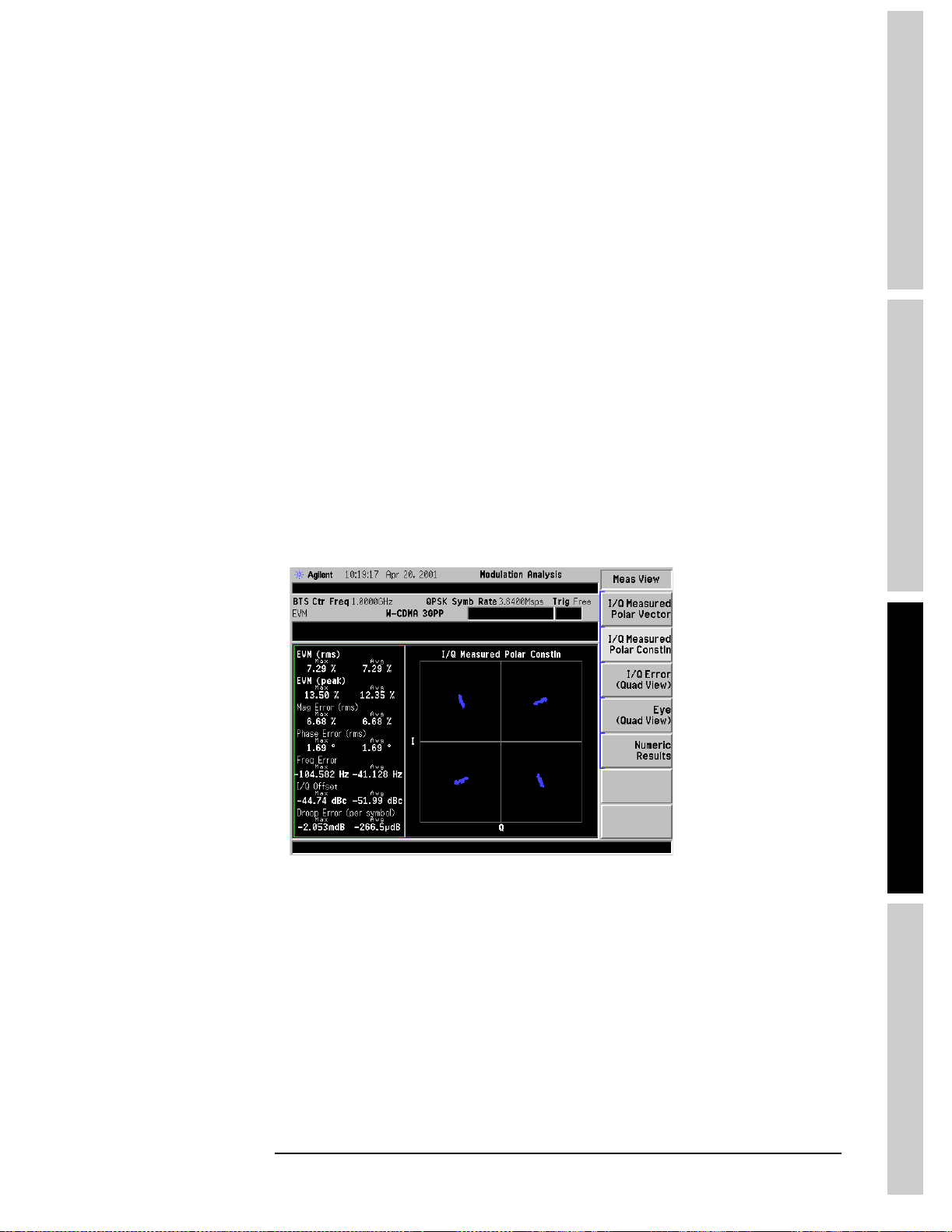
Making Modulation Analysis Measurements
A
n
a
l
y
s
s
M
o
d
e
Interpreting Measurement Results
In-Channel Amplitude Modulation Interference
Many signals are present in an integrated communications system. Examples may
include digital, baseband, IF, and RF signals. Crosstalk between adjacent
components and stages often leads to unwanted signals in the output. The
Modulation Analysis Personality can help identify these signals, including
in-channel interfering tones that are amplitude modulated.
For a Wideband CDMA signal, AM interference appears as an aligning of the
symbol decision points in the center of each quadrant, forming “lines” of dots. This
line extends farther outward as the magnitude of the AM increases.
1. Use the I/Q polar constellation diagram first to identify this problem. Press
Measured Polar Constln
CDMA signal with in-channel amplitude modulation interference. Note the
variation of amplitude around the ideal symbol reference points. Also observe
how much larger the amplitude error values are compared to those for phase
error in the table.
The results shown were created with an amplitude modulation depth of 10%
andamodulatingfrequencyof15kHz.
Figure 5-29 Polar Constellation Showing AM Interference
. Figure 5-29 shows an example of a Wideband
I/Q
Measurements
Chapter 5 81
Page 82

G
t
tngS
t
ar
ted
AnalysisM
d
M
t
Making Modulation Analysis Measurements
Interpreting Measurement Results
2. The I/Q error view graphs are shown in Figure 5-30.
e
Figure 5-30 I/Q Error Display Showing AM Interference
e
o
s
easuremen
82 Chapter 5
Page 83

Making Modulation Analysis Measurements
A
n
a
l
y
s
s
M
o
d
e
Interpreting Measurement Results
3. The zoomed phase error graph is shown in Figure 5-31. If the number of cycles
can be accurately determined, the amplitude modulating signal frequency can
be calculated. Use the
necessary, to make this determination. It may also be helpful to pause the trace
using the
AM
In this example, Phase Error freq. = 1.1 cycles, number of symbols = 256, and
symbol rate is 3.84 x 10
AMf= 1.1/256 x 3.84 x 106, or about 16 kHz
Figure 5-31 Zoomed Phase Error Display Showing AM Interference
Meas Control key.
= Phase Error freq. / number of symbols x symbol rate
f
Span and Amplitude keys to adjust the scaling, if
6
Measurements
Chapter 5 83
Page 84

G
t
tngS
t
ar
ted
AnalysisM
d
M
t
e
e
o
Making Modulation Analysis Measurements
Interpreting Measurement Results
4. Peak deviation of the amplitude modulating signal is easily determined from
Figure 5-32, the zoomed magnitude error versus time graph. There are about 7
divisions of peak-to-peak amplitude modulation at 3% per division, yielding
10.5% peak amplitude. This approximates the actual 10% of amplitude
modulation applied to create this signal.
Figure 5-32 Zoomed Magnitude Error Display Showing AM Interference
s
easuremen
84 Chapter 5
Page 85

Making Modulation Analysis Measurements
A
n
a
l
y
s
s
M
o
d
e
Interpreting Measurement Results
In-Channel Spurious Signal Interference
Many signals are present in an integrated communications system. Examples may
include digital, baseband, IF, and RF signals. Crosstalk between adjacent
components and stages often leads to unwanted signals in the output. The
Modulation Analysis Personality can help identify these signals, including
in-channel spurious signals.
For a Wideband CDMA signal, an in-channel spurious signal appears as
ring-shaped groupings of symbol decision points in each of the quadrants. This is
because the spur modulates both the amplitude and phase of the I and Q signals.
The ring diameter increases as the magnitude of the spur increases. If the signal is
modulated without spurious interference, the clusters of symbol decision points in
each quadrant will form a solid spot rather than a ring.
1. Figure 5-33 shows an in-channel spurious signal that is –15 dBc and + 400 kHz
away from the unmodulated radio signal. Even a large interfering signal such as
this is barely visible in the spectrum view, even with averaging on.
Figure 5-33 Spectrum Display Showing In-Channel Spurious Interference
Measurements
Chapter 5 85
Page 86

G
t
tngS
t
ar
ted
AnalysisM
d
M
t
e
e
o
Making Modulation Analysis Measurements
Interpreting Measurement Results
2. Use the I/Q polar constellation diagram first to identify this problem. Press I/Q
Measured Polar Constln
same interfering signal as was used in Figure 5-33.
Figure 5-34 Polar Constellation Showing Spurious Interference at –15 dBc
. Figure 5-34 shows the results created using the
3. The same view of the interfering signal is shown in Figure 5-35, but at
–28 dBc. The characteristic ring shape can still be seen.
Figure 5-35 Polar Constellation Showing Spurious Interference at –28 dBc
s
easuremen
86 Chapter 5
Page 87

Making Modulation Analysis Measurements
A
n
a
l
y
s
s
M
o
d
e
Measuring a Custom QPSK Format Signal
Measuring a Custom QPSK Format Signal
The Modulation Analysis Personality allows you to demodulate a QPSK
modulation formatted signal using your own custom parameters. This section
provides an example of how to set up the analyzer to measure such a signal. The
signal parameters are: type QPSK modulation, symbol rate 3.84 Msps, Root
Nyquist filtering using Alpha/BT of 0.35.
1. Press
2. Press
3. Press
4. Press
5. Press
6. Press
You should see the classic four symmetric decision regions (symbol points) of a
QPSK constellation, as shown in Figure 5-36.
Figure 5-36 Polar Constellation of a QPSK Signal
Demod Format, QPSK to select the correct demodulation format.
Symbol Rate, 3.84 Msps to enter the correct symbol rate.
Meas Filter, Root Nyquist to select the correct measurement filter.
Ref Filter, Nyquist to select the correct reference filter.
Det/Demod, Alpha/BT, 0.35, Enter to enter the correct alpha value.
View/Trace, I/Q Measured Polar Constln to select the correct
constellation view.
Measurements
Chapter 5 87
Page 88

G
t
tngS
t
ar
ted
AnalysisM
d
M
t
Making Modulation Analysis Measurements
Other Customized Changes You Can Make
e
Other Customized Changes You Can Make
1. Press Display to vary the number of I/Q points, I/Q points offset, and turn on or
off the symbol dots for polar vector or quad views.
2. Press
3. Set the measurement parameters to the default values by pressing
NOTE If the desired RF channel or channel frequency has been set for a previous
e
o
measurement, it is used for all subsequent measurements, and it does not need to
be set again.
4. Set the mode parameters to the default values by pressing
5. To change any of the measurement parameters from the factory default values,
Det/Demod to access a menu to allow you to vary the type of
measurement and reference filters.
Meas Setup,
More, Restore Meas Defaults
Restore Mode Setup Defaults
press the
allow you to modify the parameters for this measurement. For additional
information on keys to access measurement parameters, refer to the
Front Panel Key Reference section in this User’s Guide, or use the on-screen
help.
Meas Setup, Mode Setup,orDet/Demod keys to access menus that
.
Mode Setup,
.
s
easuremen
88 Chapter 5
Page 89

Making Modulation Analysis Measurements
A
n
a
l
y
s
s
M
o
d
e
Problems Obtaining a Measurement
Problems Obtaining a Measurement
The following list of common problems and their solutions may help if you are
having trouble obtaining a proper measurement using the Modulation Analysis
Personality.
In Monitor Spectrum mode, the signal is missing, or does not look correct
• The analyzer may be tuned to a frequency other than the radio signal frequency.
While the analyzer is in Modulation Analysis mode, press FREQUENCY
Channel
while in SA mode, the Modulation Analysis mode frequency was unaffected.
When using the GSM or EDGE standards, the spectrum looks valid, but all EVM measurements are invalid
and then set the analyzer frequency. If the analyzer frequency was set
If you are using a signal generator, the data format must be “framed” and not
“patterned,” unlike the other TDMA modes. For example, the signal needs to
be bursted with the correct midamble training sequence code as is defined in
the GSM or EDGE standard. The spectrum should look like Figure 5-37 for
both GSM and EDGE signals with only one active timeslot.
Figure 5-37 Spectrum Display of an EDGE Signal with One Active Timeslot
Measurements
Chapter 5 89
Page 90

Making Modulation Analysis Measurements
G
t
tngS
t
ted
AnalysisM
d
M
t
Problems Obtaining a Measurement
ar
e
e
o
An NADC, TETRA, or PDC signal looks incorrect
Make sure that BTS/MS is correctly selected. BTS assumes a continuous,
non-burst signal with all timeslots active.
If your NADC, TETRA or PDC BTS signal is bursted, all inactive timeslots are
transmitted as a series of the numeral 1. If fewer than six down channels (or four
for TETRA) are active, one or more of the down channels will be transmitting all
ones and the EVM results will be inaccurate. If all six down channels (or all four in
the case of TETRA) are active, this is detected as a continuous signal and can be
demodulated. The
demodulate a continuous signal.
If your NADC or PDC MS signal has two adjacent active timeslots, the signal will
be demodulated as one timeslot centered on the adjoining edges of the two
timeslots, and again the results will be inaccurate.
To alleviate the problems described above, there are several possible workarounds.
These include:
• Test your BTS signals with all timeslots active.
• Artificially create a pulse envelope by adjusting the amplitude of the timeslot
of interest.
RF Amptd parameter of Burst Sync needs to be set to None to
• Use an external trigger with
timeslots of interest.
External Trigger Delay to manually align the
A “Wideband Cal Required” error message appears
s
easuremen
•PressDet/Demod, More 1 of 2, Wideband Cal. Follow any instructions given
on the display and then continue the measurement. Once the calibration has
been completed, the analyzer will return to the previous measurement screen.
Wideband Cal allows you to perform a factory calibration of the modulation
analysis software. As the analyzer is calibrated on leaving the factory, this only
has to be done after installing new software. Calibration is best done after the
analyzer has reached its normal operating temperature. When the internal
temperature changes, a partial calibration is automatically carried out and is
indicated on the screen.
If a Wideband Cal is done when the analyzer has reached its normal operating
temperature, the number of automatic cals will be reduced. If the ESA has not
been aligned, a full Alignment is done before the Wideband Cal. Calibration is
complete once the analyzer returns to its previous screen. A Wideband Cal on
its own should take about 90 secs; a Wideband Cal with Alignment takes up to
10 mins.
90 Chapter 5
Page 91

Making Modulation Analysis Measurements
A
n
a
l
y
s
s
M
o
d
e
Problems Obtaining a Measurement
The results show a large EVM
• Make sure that the instrument reference is correct. Check if an external
reference is being used by pressing Det/Demod, More 1 of 2.Alsochecktosee
that a cable is connected between the 10 MHz OUT port of the RF
Communications Hardware (Option B7E) board to the ESA 10 MHz REF IN
port.
• When using an external reference signal, there is a possibility of significant
degradation in some EVM measurement results. This is more likely to be a
problem if your EVM measurements are being made on signals with low
symbol rates, such as TETRA, NADC or PDC. If your external reference signal
can be set to 10 MHz, connect it directly into the 10 MHz REF IN port to
alleviate this problem.
• If you are measuring a bursted signal, go to the
the burst edges are not being used in the EVM measurement. If you can see the
burst edges, you can either change the input signal properties or reduce the
Meas Interval under the Meas Setup key.
I/Q Error view and ensure that
Measurements
Chapter 5 91
Page 92

G
t
tngS
t
ar
ted
AnalysisM
d
M
t
e
e
o
Making Modulation Analysis Measurements
Problems Obtaining a Measurement
s
easuremen
92 Chapter 5
Page 93

A
n
a
l
y
s
s
M
o
d
e
M
t
6 Menu Maps
This chapter provides a visual representation of the front-panel keys and their
associated menu keys. Refer to Chapter 7 , “Front Panel Key Reference,” for key
function descriptions.
easuremen
s
93
Page 94

G
t
tngS
t
ar
ted
AnalysisM
d
M
t
Menu Maps
What You Will Find in This Chapter
e
What You Will Find in This Chapter
This chapter provides menu maps for the front panel keys having associated
menus. The key menus appear in alphabetical order as follows:
AMPLITUDE Y Scale Page 6-95
Det/Demod Page 6-96
Display Page 6-97
FREQUENCY Channel Page 6-98
e
o
Installer Page 6-99
MEASURE Page 6-100
Measurement Setup—Monitor Spectrum Page 6-101
Measurement Setup—EVM Page 6-102
MODE Page 6-103
Mode Setup Page 6-104
SPAN X Scale Page 6-105
Tri g Page 6-106
View/Trace Page 6-107
s
easuremen
94 Chapter 6
Page 95
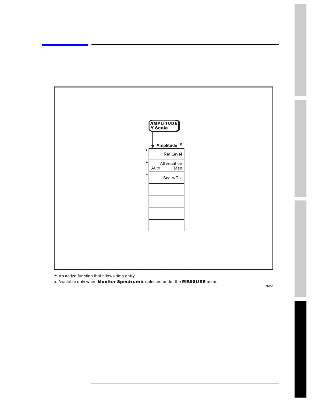
A
n
a
l
y
s
s
M
o
d
e
Menus
Amplitude Menu
Menu Maps
Menus
Measurements
Chapter 6 95
Page 96

Menu Maps
G
t
tngS
t
ted
AnalysisM
d
M
t
Menus
ar
e
e
o
Det/Demod Menus
s
easuremen
96 Chapter 6
Page 97

A
n
a
l
y
s
s
M
o
d
e
Display Menus
Menu Maps
Menus
Measurements
Chapter 6 97
Page 98

Menu Maps
G
t
tngS
t
ted
AnalysisM
d
M
t
Menus
ar
e
e
o
Frequency/Channel Menu
s
easuremen
98 Chapter 6
Page 99

Menu Maps
A
n
a
l
y
s
s
M
o
d
e
Menus
Installer Menus
For more information on the System and Personalities menus, refer to the ESA
Spectrum Analyzers User’s Guide.
Measurements
Chapter 6 99
Page 100
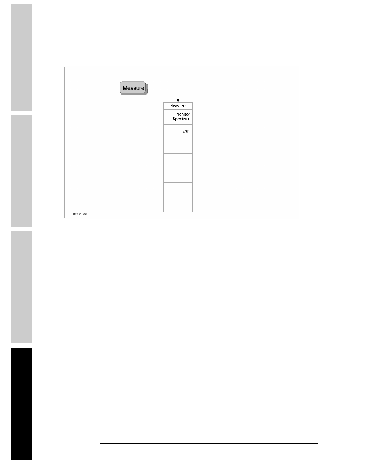
Menu Maps
G
t
tngS
t
ted
AnalysisM
d
M
t
Menus
ar
e
e
o
Measure Menu
s
easuremen
100 Chapter 6
 Loading...