Agilent E4401B Measurement Guide

Measurement Guide

Agilent Technologies ESA Spectrum Analyzers

This manual provides documentation for the following instruments:

Agilent ESA-E Series

E4401B (9 kHz – 1.5 GHz) E4402B (9 kHz – 3.0 GHz) E4404B (9 kHz – 6.7 GHz) E4405B (9 kHz – 13.2 GHz) E4407B (9 kHz – 26.5 GHz)

and

Agilent ESA-L Series

E4411B (9 kHz – 1.5GHz) E4403B (9 kHz – 6.7 GHz) E4408B (9 kHz – 26.5 GHz)

Manufacturing Part Number: E4401-90175

Supersedes E4401-90111

Printed in USA

March 2000

The information contained in this document is subject to change without notice.

Agilent Technologiesmakesnowarrantyofanykindwithregard to this material, including but not limited to, the implied warranties of merchantability and ﬁtness for a particular purpose. Agilent Technologies shall not be liable for errors contained herein or for incidental or consequential damages in connection with the furnishing, performance, or use of this material.

The following safety symbols are used throughout this manual. Familiarize yourself with the symbols and their meaning before operating this instrument.

WARNING Warning denotes a hazard. It calls attention to a procedure

which, if not correctly performed or adhered to, could result in injury or loss of life. Do not proceed beyond a warning note until the indicated conditions are fully understood and met.

CAUTION Caution denotes a hazard. It calls attention to a procedure that, if not

correctly performed or adhered to, could result in damage to or destruction of the instrument. Do not proceed beyond a caution sign until the indicated conditions are fully understood and met.

NOTE Note calls out special information for the user’s attention. It provides

operational information or additional instructions of which the user should be aware.

The instruction documentation symbol. The product is marked with this symbol when it is necessary for the user to refer to the instructions in the documentation.

This symbol is used to mark the on position of the power line switch.

This symbol is used to mark the standby position of the power line switch.

This symbol indicates that the input power required is AC.

WARNING This is a Safety Class 1 Product (provided with a protective

earthing ground incorporated in the power cord). The mains plug shall only be inserted in a socket outlet provided with a protected earth contact. Any interruption of the protective conductor inside or outside of the product is likely to make the product dangerous. Intentional interruption is prohibited.

WARNING If this product is not used as speciﬁed, the protection provided

by the equipment could be impaired. This product must be used in a normal condition (in which all means for protection are intact) only.

Warranty

This Agilent Technologies instrument product is warranted against defects in material and workmanship for a period of three years from date of shipment. During the warranty period, Agilent Technologies will, at its option, either repair or replace products which prove to be defective.

For warranty service or repair, this product must be returned to a service facility designated by Agilent Technologies. Buyer shall prepay shipping charges to Agilent Technologies and Agilent Technologies shall pay shipping charges to return the product to Buyer. However, Buyer shall pay all shipping charges, duties, and taxes for products returned to Agilent Technologies from another country.

Agilent Technologies warrants that its software and ﬁrmware designated by Agilent Technologies for use with an instrument will execute its programming instructions when properly installed on that instrument. Agilent Technologies does not warrant that the operation of the instrument, or software, or ﬁrmware will be uninterrupted or error-free.

LIMITATION OF WARRANTY

The foregoing warranty shall not apply to defects resulting from improper or inadequate maintenance by Buyer, Buyer-supplied software or interfacing, unauthorized modiﬁcation or misuse, operation outside of the environmental speciﬁcations for the product, or improper site preparation or maintenance.

NO OTHER WARRANTY IS EXPRESSED OR IMPLIED. AGILENT TECHNOLOGIES SPECIFICALLY DISCLAIMS THE IMPLIED WARRANTIES OF MERCHANTABILITY AND FITNESS FOR A PARTICULAR PURPOSE.

iii

EXCLUSIVE REMEDIES

THE REMEDIES PROVIDED HEREIN ARE BUYER’S SOLE AND EXCLUSIVE REMEDIES. AGILENT TECHNOLOGIES SHALL NOT BE LIABLE FOR ANY DIRECT, INDIRECT, SPECIAL, INCIDENTAL, OR CONSEQUENTIAL DAMAGES, WHETHER BASED ON CONTRACT, TORT, OR ANY OTHER LEGAL THEORY.

Where to Find the Latest Information

Documentation is updated periodically.For the latest information about Agilent ESA Spectrum Analyzers, including ﬁrmware upgrades and application information, please visit the following Internet URL:

http://www.agilent.com/ﬁnd/esa

1. Making Basic Measurements

What is in This Chapter . . . . . . . . . . . . . . . . . . . . . . . . . . . . . . . . . . . . . . . . . . . . . . . . . . . . . .1-2

Comparing Signals . . . . . . . . . . . . . . . . . . . . . . . . . . . . . . . . . . . . . . . . . . . . . . . . . . . . . . . . . .1-3

Example 1:. . . . . . . . . . . . . . . . . . . . . . . . . . . . . . . . . . . . . . . . . . . . . . . . . . . . . . . . . . . . . . . .1-3

Example 2:. . . . . . . . . . . . . . . . . . . . . . . . . . . . . . . . . . . . . . . . . . . . . . . . . . . . . . . . . . . . . . . .1-5

Resolving Signals of Equal Amplitude . . . . . . . . . . . . . . . . . . . . . . . . . . . . . . . . . . . . . . . . . . .1-6

Example: . . . . . . . . . . . . . . . . . . . . . . . . . . . . . . . . . . . . . . . . . . . . . . . . . . . . . . . . . . . . . . . . .1-7

Resolving Small Signals Hidden by Large Signals . . . . . . . . . . . . . . . . . . . . . . . . . . . . . . . . .1-9

Example: . . . . . . . . . . . . . . . . . . . . . . . . . . . . . . . . . . . . . . . . . . . . . . . . . . . . . . . . . . . . . . . .1-10

Making Better Frequency Measurements . . . . . . . . . . . . . . . . . . . . . . . . . . . . . . . . . . . . . . .1-12

Example: . . . . . . . . . . . . . . . . . . . . . . . . . . . . . . . . . . . . . . . . . . . . . . . . . . . . . . . . . . . . . . . .1-12

Decreasing the Frequency Span Around the Signal . . . . . . . . . . . . . . . . . . . . . . . . . . . . . . .1-14

Example: . . . . . . . . . . . . . . . . . . . . . . . . . . . . . . . . . . . . . . . . . . . . . . . . . . . . . . . . . . . . . . . .1-14

Tracking Drifting Signals . . . . . . . . . . . . . . . . . . . . . . . . . . . . . . . . . . . . . . . . . . . . . . . . . . . .1-16

Example 1:. . . . . . . . . . . . . . . . . . . . . . . . . . . . . . . . . . . . . . . . . . . . . . . . . . . . . . . . . . . . . . .1-16

Example 2:. . . . . . . . . . . . . . . . . . . . . . . . . . . . . . . . . . . . . . . . . . . . . . . . . . . . . . . . . . . . . . .1-18

Measuring Low Level Signals . . . . . . . . . . . . . . . . . . . . . . . . . . . . . . . . . . . . . . . . . . . . . . . . .1-20

Example 1:. . . . . . . . . . . . . . . . . . . . . . . . . . . . . . . . . . . . . . . . . . . . . . . . . . . . . . . . . . . . . . .1-20

Example 2:. . . . . . . . . . . . . . . . . . . . . . . . . . . . . . . . . . . . . . . . . . . . . . . . . . . . . . . . . . . . . . .1-23

Example 3:. . . . . . . . . . . . . . . . . . . . . . . . . . . . . . . . . . . . . . . . . . . . . . . . . . . . . . . . . . . . . . .1-24

Example 4:. . . . . . . . . . . . . . . . . . . . . . . . . . . . . . . . . . . . . . . . . . . . . . . . . . . . . . . . . . . . . . .1-26

Identifying Distortion Products . . . . . . . . . . . . . . . . . . . . . . . . . . . . . . . . . . . . . . . . . . . . . . .1-28

Distortion from the Analyzer . . . . . . . . . . . . . . . . . . . . . . . . . . . . . . . . . . . . . . . . . . . . . . . .1-28

Third-Order Intermodulation Distortion . . . . . . . . . . . . . . . . . . . . . . . . . . . . . . . . . . . . . .1-31

Measuring Signal-to-Noise . . . . . . . . . . . . . . . . . . . . . . . . . . . . . . . . . . . . . . . . . . . . . . . . . . .1-34

Making Noise Measurements . . . . . . . . . . . . . . . . . . . . . . . . . . . . . . . . . . . . . . . . . . . . . . . . .1-36

Example 1:. . . . . . . . . . . . . . . . . . . . . . . . . . . . . . . . . . . . . . . . . . . . . . . . . . . . . . . . . . . . . . .1-36

Example 2:. . . . . . . . . . . . . . . . . . . . . . . . . . . . . . . . . . . . . . . . . . . . . . . . . . . . . . . . . . . . . . .1-38

Example 3:. . . . . . . . . . . . . . . . . . . . . . . . . . . . . . . . . . . . . . . . . . . . . . . . . . . . . . . . . . . . . . .1-39

Example 4:. . . . . . . . . . . . . . . . . . . . . . . . . . . . . . . . . . . . . . . . . . . . . . . . . . . . . . . . . . . . . . .1-41

Demodulating AM Signals (Using the Analyzer As a Fixed Tuned Receiver) . . . . . . . . . . .1-43

Example: . . . . . . . . . . . . . . . . . . . . . . . . . . . . . . . . . . . . . . . . . . . . . . . . . . . . . . . . . . . . . . . .1-43

Demodulating FM Signals

(Without Option BAA) . . . . . . . . . . . . . . . . . . . . . . . . . . . . . . . . . . . . . . . . . . . . . . . . . . . . . . .1-46

Example: . . . . . . . . . . . . . . . . . . . . . . . . . . . . . . . . . . . . . . . . . . . . . . . . . . . . . . . . . . . . . . . .1-46

2. Making Measurements

What’s in This Chapter . . . . . . . . . . . . . . . . . . . . . . . . . . . . . . . . . . . . . . . . . . . . . . . . . . . . . . .2-2

Making Stimulus Response Measurements . . . . . . . . . . . . . . . . . . . . . . . . . . . . . . . . . . . . . . .2-3

What Are Stimulus Response Measurements? . . . . . . . . . . . . . . . . . . . . . . . . . . . . . . . . . .2-3

Using An Analyzer With A Tracking Generator. . . . . . . . . . . . . . . . . . . . . . . . . . . . . . . . . .2-3

Stepping Through a Transmission Measurement. . . . . . . . . . . . . . . . . . . . . . . . . . . . . . . . .2-4

Tracking Generator Unleveled Condition . . . . . . . . . . . . . . . . . . . . . . . . . . . . . . . . . . . . . . .2-8

Measuring Device Bandwidth . . . . . . . . . . . . . . . . . . . . . . . . . . . . . . . . . . . . . . . . . . . . . . . .2-9

Making a Reﬂection Calibration Measurement . . . . . . . . . . . . . . . . . . . . . . . . . . . . . . . . . . .2-12

Example: . . . . . . . . . . . . . . . . . . . . . . . . . . . . . . . . . . . . . . . . . . . . . . . . . . . . . . . . . . . . . . . .2-13

Reﬂection Calibration . . . . . . . . . . . . . . . . . . . . . . . . . . . . . . . . . . . . . . . . . . . . . . . . . . . . .2-13

Measuring the Return Loss . . . . . . . . . . . . . . . . . . . . . . . . . . . . . . . . . . . . . . . . . . . . . . . . .2-14

Demodulating and Listening to an AM Signal . . . . . . . . . . . . . . . . . . . . . . . . . . . . . . . . . . .2-15

Contents

Example 1: . . . . . . . . . . . . . . . . . . . . . . . . . . . . . . . . . . . . . . . . . . . . . . . . . . . . . . . . . . . . . . 2-15

Example 2: . . . . . . . . . . . . . . . . . . . . . . . . . . . . . . . . . . . . . . . . . . . . . . . . . . . . . . . . . . . . . . 2-17

Measuring Harmonics and Harmonic Distortion . . . . . . . . . . . . . . . . . . . . . . . . . . . . . . . . .2-19

Example:. . . . . . . . . . . . . . . . . . . . . . . . . . . . . . . . . . . . . . . . . . . . . . . . . . . . . . . . . . . . . . . . 2-20

Demodulating and Viewing Television Signals

(Option B7B) . . . . . . . . . . . . . . . . . . . . . . . . . . . . . . . . . . . . . . . . . . . . . . . . . . . . . . . . . . . . . . 2-25

Example 1: . . . . . . . . . . . . . . . . . . . . . . . . . . . . . . . . . . . . . . . . . . . . . . . . . . . . . . . . . . . . . . 2-25

Example 2: . . . . . . . . . . . . . . . . . . . . . . . . . . . . . . . . . . . . . . . . . . . . . . . . . . . . . . . . . . . . . . 2-29

TV Trig Setup Menu Functions. . . . . . . . . . . . . . . . . . . . . . . . . . . . . . . . . . . . . . . . . . . . . . 2-30

Using External Millimeter Mixers

(Option AYZ) . . . . . . . . . . . . . . . . . . . . . . . . . . . . . . . . . . . . . . . . . . . . . . . . . . . . . . . . . . . . . . 2-33

Example 1: Making measurements with unpreselected millimeter-wave mixers . . . . . . 2-33

Example 2: Making Measurements with HP/Agilent 11974 Series Preselected

Millimeter-Wave Mixers. . . . . . . . . . . . . . . . . . . . . . . . . . . . . . . . . . . . . . . . . . . . . . . . . . . . 2-37

1 Making Basic Measurements

1-1

Making Basic Measurements

What is in This Chapter

This chapter demonstrates basic analyzer measurements with examples of typical measurements; each measurement focuses on different functions. The measurement procedures covered in this chapter are listed below.

• “Comparing Signals” on page 1-3

• “Resolving Signals of Equal Amplitude” on page 1-6

• “Resolving Small Signals Hidden by Large Signals” on page 1-9

• “Making Better Frequency Measurements” on page 1-12

• “Decreasing the Frequency Span Around the Signal” on page 1-14

• “Tracking Drifting Signals” on page 1-16

• “Measuring Low Level Signals” on page 1-20

• “Identifying Distortion Products” on page 1-28

• “Measuring Signal-to-Noise” on page 1-34

• “Making Noise Measurements” on page 1-36

• “Demodulating AM Signals (Using the Analyzer As a Fixed Tuned

Receiver)” on page 1-43

• “Demodulating FM Signals (Without Option BAA)” on page 1-46

To ﬁnd descriptions of speciﬁc analyzer functions, refer to the user’s guide.

1-2 Chapter1

Making Basic Measurements

Comparing Signals

Using the analyzer, you can easily compare frequency and amplitude differences between signals, such as radio or television signal spectra. The analyzer delta marker function lets you compare two signals when both appear on the screen at one time or when only one appears on the screen.

Example 1:

Measure the differences between two signals on the same display screen.

1. Connect the 10 MHz REF OUT from the rear panel to the front-panel INPUT.

2. Set the center frequency to 30 MHz and the span to 50 MHz by pressing

FREQUENCY, 30 MHz, SPAN, 50 MHz.

3. Set the reference level to 10 dBm by pressing The 10 MHz reference signal and its harmonics appear on the

display.

4. Press display. (The

Peak Search to place a marker at the highest peak on the

Next Peak, Next Pk Right and Next Pk Left keys are

available to move the marker from peak to peak.) The marker should be on the 10 MHz reference signal. See Figure 1-1.

Figure 1-1 Placing a Marker on the 10 MHz Signal

AMPLITUDE, 10 dBm.

Chapter 1 1-3

Making Basic Measurements

Comparing Signals

5. Press Marker, Delta, to activate a second marker at the position of the ﬁrst marker. Move the second marker to another signal peak using the knob, or by pressing

Next Pk Left.

Peak Search and Next Peak, Next Pk Right or

6. The amplitude and frequency difference between the markers is displayed in the active function block and in the upper right corner of the screen. See Figure 1-2. The resolution of the marker readings can be increased by turning on the frequency count function. Press

Freq Count. Both signals are counted.

Press

Marker, Off to turn the markers off.

Figure 1-2 Using the Marker Delta Function

1-4 Chapter1

Making Basic Measurements

Comparing Signals

Example 2:

Measure the frequency and amplitude difference between two signals that do not appear on the screen at one time. (This technique is useful for harmonic distortion tests when narrow span and narrow bandwidth are necessary to measure the low level harmonics.)

1. Connect the 10 MHz REF OUT from the rear panel to the front-panel INPUT.

2. Set the center frequency to 10 MHz and the span to 5 MHz by pressing

FREQUENCY, 10 MHz, SPAN, 5 MHz.

3. Set the reference level to 10 dBm by pressing

4. Press

5. Press

Peak Search to place a marker on the peak. Marker→, Mkr→CF Step to set the center frequency step size

AMPLITUDE, 10 dBm.

equal to the frequency of the fundamental signal.

6. Press Marker, Delta to anchor the position of the ﬁrst marker and activate a second marker.

7. Press FREQUENCY, Center Freq and the (↑) key to increase the center frequency by 10 MHz. The ﬁrst marker remains on the screen at the amplitude of the ﬁrst signal peak.

The annotation in the upper right corner of the screen indicates the amplitude and frequency difference between the two markers. See

Figure 1-3.

8. To turn the markers off, press

Marker, Off.

Figure 1-3 Frequency and Amplitude Difference Between Signals

Chapter 1 1-5

Making Basic Measurements

Resolving Signals of Equal Amplitude

Two equal-amplitude input signals that are close in frequency can appear as one on the analyzer display. Responding to a single-frequency signal, a swept-tuned analyzer traces out the shape of the selected internal IF (intermediate frequency) ﬁlter. As you change the ﬁlter bandwidth, you change the width of the displayed response. If a wide ﬁlter is used and two equal-amplitude input signals are close enough in frequency, then the two signals appear as one. Thus, signal resolution is determined by the IF ﬁlters inside the analyzer.

The bandwidth of the IF ﬁlter tells us how close together equal amplitude signals can be and still be distinguished from each other. The resolution bandwidth function selects an IF ﬁlter setting for a measurement. Resolution bandwidth is deﬁned as the 3 dB bandwidth of the ﬁlter.

Generally, to resolve two signals of equal amplitude, the resolution bandwidth must be less than or equal to the frequency separation of the two signals. If the bandwidth is equal to the separation and the video bandwidth is less than the resolution bandwidth, a dip of approximately 3 dB is seen between the peaks of the two equal signals, and it is clear that more than one signal is present. See Figure 1-5.

In order to keep the analyzer measurement calibrated, sweep time is automatically set to a value that is inversely proportional to the square of the resolution bandwidth (for resolution bandwidths ≥ 1kHz). So, if the resolution bandwidth is reduced by a factor of 10, the sweep time is increased by a factor of 100 when sweep time and bandwidth settings

are coupled. (Sweep time is proportional to

1/BW

.) For shortest measurement times, use the widest resolution bandwidth that still permits discrimination of all desired signals.The analyzer allows you to select from 1 kHz to 3 MHz resolution bandwidths in a 1, 3, 10 sequence and 5 MHz for maximum measurement ﬂexibility.

Option 1DR adds narrower resolution bandwidths, from 10 Hz to 300 Hz, in a 1-3-10 sequence. These bandwidths are digitally implemented and have a much narrower shape factor than the wider, analog resolution bandwidths. Also, the autocoupled sweeptimes when using the digital resolution bandwidths are much faster than analog bandwidths of the same width.

1-6 Chapter1

Example:

Resolve two signals of equal amplitude with a frequency separation of 100 kHz.

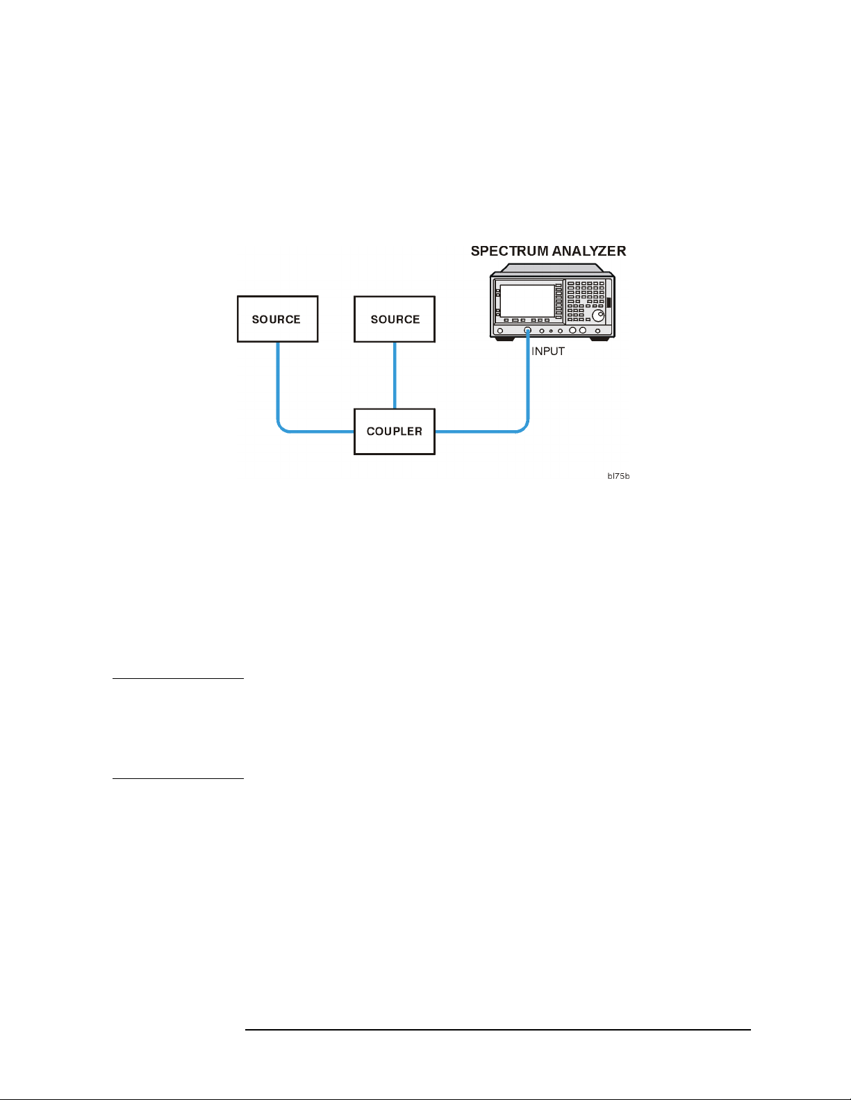
1. Connect two sources to the analyzer input as shown in Figure 1-4.

Figure 1-4 Setup for Obtaining Two Signals

Making Basic Measurements

Resolving Signals of Equal Amplitude

2. Set one source to 300 MHz. Set the frequency of the other source to

300.1 MHz. The amplitude of both signals should be approximately

−20 dBm.

3. On the analyzer, press

Preset, Factory Preset (softkey), if present. Set

the center frequency to 300 MHz, the span to 2 MHz, and the resolution bandwidth to 300 kHz by pressing

SPAN, 2 MHz, then BW/Avg, Resolution BW, 300 kHz. A single signal

FREQUENCY, 300 MHz,

peak is visible.

NOTE If the signal peak cannot be found, increase the span to 20 MHz by

pressing

FREQUENCY, Signal Track (On), then SPAN, 2 MHz to bring the signal to

center screen. Then press

SPAN, 20 MHz. The signal should be visible. Press Search,

Signal Track (Off) to turn the signal track

function off.

4. Since the resolution bandwidth must be less than or equal to the frequency separation of the two signals, a resolution bandwidth of 100 kHz must be used. Change the resolution bandwidth to 100 kHz by pressing

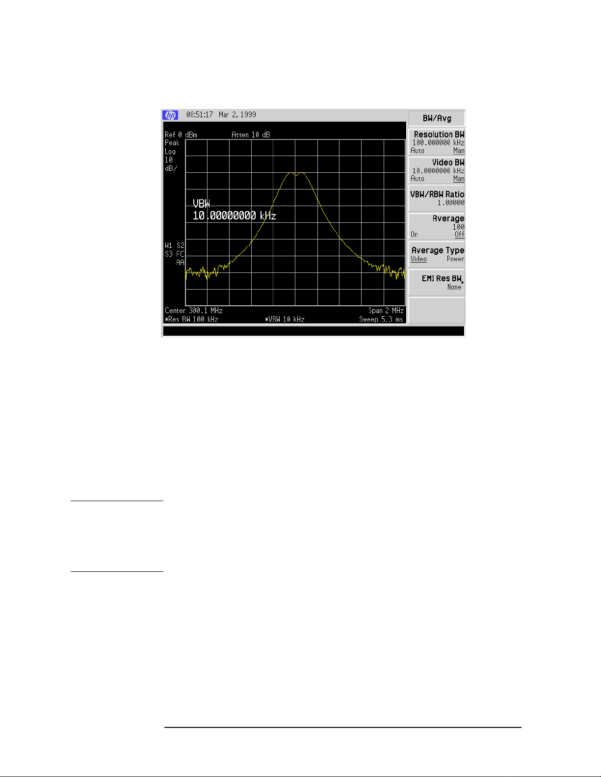
BW/Avg, 100 kHz. Two signals are now visible as shown in

Figure 1-5. Use the knob or step keys to further reduce the

resolution bandwidth and better resolve the signals.

5. Decrease the video bandwidth to 10 kHz, by pressing

Video BW (Man), 10 kHz.

Chapter 1 1-7

Making Basic Measurements

Resolving Signals of Equal Amplitude

Figure 1-5 Resolving Signals of Equal Amplitude

As the resolution bandwidth is decreased, resolution of the individual signals is improved and the sweep time is increased. For fastest measurement times, use the widest possible resolution bandwidth. Under factory preset conditions, the resolution bandwidth is “coupled” (or linked) to the span.

Since the resolution bandwidth has been changed from the coupled value, a # mark appears next to Res BW in the lower-left corner of the screen, indicating that the resolution bandwidth is uncoupled. (Also see the

Auto Couple key description in the user’s guide.)

NOTE To resolve two signals of equal amplitude with a frequency separation

of 200 kHz, the resolution bandwidth must be less than the signal separation, and resolution of 100 kHz must be used. The next larger ﬁlter, 300 kHz, would exceed the 200 kHz separation and would not resolve the signals.

1-8 Chapter1

Making Basic Measurements

Resolving Small Signals Hidden by Large Signals

When dealing with the resolution of signals that are close together and not equal in amplitude, you must consider the shape of the IF ﬁlter of the analyzer, as well as its 3 dB bandwidth. (See “Resolving Signals of

Equal Amplitude” on page 1-6 example for more information.) The

shape of a ﬁlter is deﬁned by the selectivity, which is the ratio of the 60 dB bandwidth to the 3 dB bandwidth. (Generally, the IF ﬁlters in this analyzer have shape factors of 15:1 or less for resolution bandwidths ≥1kHz and 5:1 or less for resolution bandwidths ≤ 300 Hz). If a small signal is too close to a larger signal, the smaller signal can be hidden by the skirt of the larger signal. To view the smaller signal, you must select a resolution bandwidth such that k is less than a. See

Figure 1-6.

Figure 1-6 Resolution Bandwidth Requirements for Resolving Small

Signals

The separation between the two signals (a) must be greater than half the ﬁlter width of the larger signal (k) measured at the amplitude level of the smaller signal.

Chapter 1 1-9

Making Basic Measurements

Resolving Small Signals Hidden by Large Signals

Example:

Resolve two input signals with a frequency separation of 155 kHz and an amplitude separation of 60 dB.

1. To obtain two signals with a 155 kHz separation, connect the equipment as shown in the previous section, “Resolving Signals of

Equal Amplitude” on page 1-6. Set one source to 300 MHz at

−20 dBm.

2. Set the analyzer center frequency to 300 MHz and the span to 2 MHz: press

NOTE If the signal peak cannot be found, increase the span to 20 MHz by

pressing

FREQUENCY, Signal Track (On), then SPAN, 2 MHz to bring the signal to

SPAN, 20 MHz. The signal should be visible. Press Search,

center screen. Then press function off.

3. Set the second source to 300.155 MHz, so that the signal is 155 kHz higher than the ﬁrst signal. Set the amplitude of the signal to

−80 dBm (60 dB below the ﬁrst signal).

FREQUENCY, 300 MHz, then SPAN, 2 MHz.

Signal Track (Off) to turn the signal track

4. Set the 300 MHz signal to the reference level by pressing

Search, Meas Tools, then Mkr → Ref Lvl.

5. Place a marker on the smaller signal by pressing

Delta, Next Pk Right.

Peak

If a 10 kHz ﬁlter with a typical shape factor of 15:1 is used, the ﬁlter will have a bandwidth of 150 kHz at the 60 dB point. The half-bandwidth (75 kHz) is narrower than the frequency separation, so the input signals will be resolved. See Figure 1-7.

1-10 Chapter1

Making Basic Measurements

Resolving Small Signals Hidden by Large Signals

Figure 1-7 Signal Resolution with a 10 kHz Resolution Bandwidth

If a 30 kHz ﬁlter is used, the 60 dB bandwidth could be as wide as 450 kHz. Since the half-bandwidth (225 kHz) is wider than the frequency separation, the signals most likely will not be resolved. See

Figure 1-8. (In this example, we used the 60 dB bandwidth value. To

determine resolution capability for intermediate values of amplitude level differences, assume the ﬁlter skirts between the 3 dB and 60 dB points are approximately straight.)

Figure 1-8 Signal Resolution with a 30 kHz Resolution Bandwidth

Chapter 1 1-11

Making Basic Measurements

Making Better Frequency Measurements

A built-in frequency counter increases the resolution and accuracy of the frequency readout. When using this function, if the ratio of the resolution bandwidth to the span is too small (less than 0.002), the Marker Count: Widen Res BW message appears on the display. It indicates that the resolution bandwidth is too narrow.

Example:

Increase the resolution and accuracy of the frequency readout on the signal of interest.

1. Turn on the internal 50 MHz alignment signal of the analyzer (if you have not already done so).

For the E4401B and E4411B, use the internal 50 MHz alignment signal of the analyzer as the signal being measured. Press

Factory Preset (if present), Input/Output, Amptd Ref (On).

Preset,

Forall other models connect a cable between the front-panel AMPTD REF OUT to the analyzer INPUT, then press Preset, Factory Preset (if displayed), Input/Output, Amptd Ref Out (On).

2. Set the center frequency to 50 MHz by pressing

3. Set the span to 80 MHz by pressing

4. Press

Freq Count. (Note that Marker Count On Off has On

SPAN, 80 MHz.

FREQUENCY, 50 MHz.

underlined turning the frequency counter on.) The frequency and amplitude of the marker and the word Marker will appear in the active function area (this is not the counted result). The counted result appears in the upper-right corner of the display.

5. Move the marker,with the front-panel knob, half-way down the skirt of the signal response. Notice that the readout in the active function changes while the counted result (upper-right corner of display) does not. See Figure 1-9. To get an accurate count, you do not need to place the marker at the exact peak of the signal response.

NOTE Marker count properly functions onlyon CW signals or discrete spectral

components. Marker must be >26 dB above the noise.

6. Increase the counter resolution by pressing

Resolution (Man) and

then entering the desired resolution using the step keys or the numbers keypad. For example, press 1 kHz. The marker counter readout is in the upper-right corner of the screen. The resolution can be set from 1 Hz to 100 kHz.

1-12 Chapter1

7. The marker counter remains on until turned off.Turn off the marker counter by pressing

Freq Count, then Marker Count (Off). Marker, Off

also turns the marker counter off.

Figure 1-9 Using Marker Counter

Making Basic Measurements

Making Better Frequency Measurements

Chapter 1 1-13

Making Basic Measurements

Decreasing the Frequency Span Around the Signal

Using the analyzer signal track function, you can quickly decrease the span while keeping the signal at center frequency. This is a fast way to take a closer look at the area around the signal to identify signals that would otherwise not be resolved.

Example:

Examine a signal in a 200 kHz span.

1. Turn on the internal 50 MHz alignment signal of the analyzer (if you have not already done so).

For the E4401B and E4411B, use the internal 50 MHz alignment signal of the analyzer as the signal being measured. Press

Factory Preset (if present), Input/Output, Amptd Ref (On).

Preset,

Forall other models connect a cable between the front-panel AMPTD REF OUT to the analyzer INPUT, then press Preset, Factory Preset (if present), Input/Output, Amptd Ref Out (On).

2. Set the stop frequency to 1 GHz by pressing

1 GHz.

3. Press

4. Press

Peak Search to place a marker at the peak. FREQUENCY, Signal Track (On) and the signal will move to the

FREQUENCY, Stop Freq,

center of the screen, if it is not already positioned there. (Note that the marker must be on the signal before turning signal track on.) Because the signal track function automatically maintains the signal at the center of the screen, you can reduce the span quickly for a closer look. If the signal drifts off of the screen as you decrease the span, use a wider frequency span.

5. Press

SPAN, 200 kHz. The span decreases in steps as automatic zoom

is completed. See Figure 1-10. You can also use the knob or step keys to decrease the span or use the

Press

NOTE When you are ﬁnished with the example, turn off the signal tracking

Signal Track (Off) again to turn off the signal track function.

Span Zoom function under SPAN.

function.

1-14 Chapter1

Decreasing the Frequency Span Around the Signal

Figure 1-10 After Zooming In on the Signal

Making Basic Measurements

Chapter 1 1-15

Making Basic Measurements

Tracking Drifting Signals

The signal track function is useful for tracking drifting signals that drift relatively slowly.

Signal Track On Off may be used to track these drifting signals. Use Peak Search to place a marker on the signal you wish to track. Pressing FREQUENCY, Signal Track (On) will bring that signal to the center

frequency of the graticule and adjust the center frequency every sweep to bring the selected signal back to the center. ( menu, is a quick way to perform the Search, FREQUENCY, Signal Track

On Off, SPAN key sequence.)

Note that the primary function of the signal track function is to track unstable signals, not to track a signal as the center frequency of the analyzer is changed. If you choose to use the signal track function when changing center frequency, check to ensure that the signal found by the tracking function is the correct signal.

Span Zoom, in the SPAN

Example 1:

Use the signal track function to keep a drifting signal at the center of the display and monitor its change.

This example requires a signal generator. The frequency of the signal generator will be changed while you view the signal on the display of the analyzer.

1. Connect a signal generator to the analyzer input. Press

Factory Preset (if present).

2. Set the signal generator frequency to 300 MHz with an amplitude of

−20 dBm.

3. Set the center frequency of the analyzer to 300 MHz by pressing

FREQUENCY, 300 MHz.

4. Press

5. Set the span to 10 MHz by pressing

6. Press

Marker and move the marker to the peak of your signal.

SPAN, 10 MHz.

SPAN, Span Zoom, 500 kHz.

Notice that the signal has been held in the center of the display.

Preset,

1-16 Chapter1

Making Basic Measurements

Tracking Drifting Signals

7. The signal frequency drift can be read from the screen if both the signal track and marker delta functions are active. Press

Delta. The marker readout indicates the change in frequency and

amplitude as the signal drifts.

8. Tune the frequency of the signal generator. Notice that the center frequency of the analyzer changes in < 10 kHz increments,centering the signal with each increment. See Figure 1-11.

Figure 1-11 Using Signal Tracking to Track a Drifting Signal

Marker,

Chapter 1 1-17

Making Basic Measurements

Tracking Drifting Signals

Example 2:

The analyzer can measure the short and long-term stability of a source. The maximum amplitude level and the frequency drift of an input signal trace can be displayed and held by using the maximum-hold function. You can also use the maximum hold function if you want to determine how much of the frequency spectrum a signal occupies.

1. Connect a signal generator to the analyzer input. Press

Factory Preset (if present).

Preset,

2. Set the signal generator frequency to 300 MHz with an amplitude of

−20 dBm.

3. Set the center frequency of the analyzer to 300 MHz by pressing

FREQUENCY, 300 MHz.

4. Press

5. Set the span to 10 MHz by pressing

6. Press

7. Turn off the signal track function by pressing

Track (Off).

8. To measure the excursion of the signal, press

Hold. As the signal varies, maximum hold maintains the maximum

Marker and move the marker to the peak of your signal.

SPAN, 10 MHz.

SPAN, Span Zoom, 500 kHz.

FREQUENCY, Signal

View/Trace then Max

responses of the input signal. Annotation on the left side of the screen indicates the trace mode.

For example, M1 S2 S3 indicates trace 1 is in maximum-hold mode, trace 2 and trace 3 are in store- blank mode. See “Display Annotation” in Chapter 2 of the User’s Guide.

9. Press when 2 is underlined.) Press

View/Trace, Trace 1 2 3, to select trace 2. (Trace 2 is selected

Clear Write to place trace 2 in clear-write

mode, which displays the current measurement results as it sweeps. Trace 1 remains in maximum hold mode, showing the frequency shift of the signal.

Slowly change the frequency of the signal generator ± 50 kHz. Your analyzer display should look similar to Figure 1-12.

1-18 Chapter1

Making Basic Measurements

Tracking Drifting Signals

Figure 1-12 Viewing a Drifting Signal With Max Hold and Clear Write

Chapter 1 1-19

Making Basic Measurements

Measuring Low Level Signals

The ability of the analyzer to measure low level signals is limited by the noise generated inside the analyzer. A signal may be masked by the noise ﬂoor so that it is not visible. This sensitivity to low level signals is affected by the measurement setup.

The analyzer input attenuator and bandwidth settings affect the sensitivity by changing the signal-to-noise ratio. The attenuator affects the level of a signal passing through the instrument, whereas the bandwidth affects the level of internal noise without affecting the signal. In the ﬁrst two examples in this section, the attenuator and bandwidth settings are adjusted to view low level signals.

If, after adjusting the attenuation and resolution bandwidth, a signal is still near the noise, visibility can be improved by using the video bandwidth and video averaging functions, as demonstrated in the third and fourth examples.

Example 1:

If a signal is very close to the noise ﬂoor, reducing input attenuation brings the signal out of the noise. Reducing the attenuation to 0 dB maximizes signal power in the analyzer.

CAUTION The total power of all input signals at the analyzer input must not

exceed the maximum power level for the analyzer.

1. Connect a signal generator to the analyzer input. Press

Factory Preset (if present).

2. Set the signal generator frequency to 300 MHz with an amplitude of

−80 dBm.

3. Set the center frequency of the analyzer to 300 MHz by pressing

FREQUENCY, 300 MHz.

4. Set the span to 5 MHz by pressing

5. Set the reference level to −40 dBm by pressing

40 −dBm.

6. Place the signal at center frequency by pressing

Tools, Mkr→CF.

SPAN, 5 MHz.

AMPLITUDE, Ref Level,

Peak Search, Meas

Preset,

7. Reduce the span to 1 MHz. Press

SPAN, and then use the step-down

key (↓). See Figure 1-13.

1-20 Chapter1

Figure 1-13 Low-Level Signal

Making Basic Measurements

Measuring Low Level Signals

8. Press

AMPLITUDE, Attenuation (Man). Press the step-up key (↑) twice

to select 20 dB attenuation. Increasing the attenuation moves the noise ﬂoor closer to the signal.

A # mark appears next to the Atten annotation at the top of the display, indicating the attenuation is no longer coupled to other analyzer settings.

9. To see the signal more clearly, enter 0 dB. Zero attenuation makes the signal more visible. See Figure 1-14.

Before connecting other signals to the analyzer input, increase the RF attenuation to protect the analyzer input: press press

Auto Couple.

Attenuation (Auto) or

Chapter 1 1-21

Making Basic Measurements

Measuring Low Level Signals

Figure 1-14 Using 0 dB Attenuation

1-22 Chapter1

Making Basic Measurements

Measuring Low Level Signals

Example 2:

The resolution bandwidth can be decreased to view low level signals.

1. As in the previous example, set the analyzer to view a low level signal. Connect a signal generator to the analyzer input. Press

Preset, Factory Preset (if present).

2. Set the signal generator frequency to 300 MHz with an amplitude of

−80 dBm.

3. Set the center frequency of the analyzer to 300 MHz by pressing

FREQUENCY, 300 MHz.

4. Set the span to 5 MHz by pressing

5. Set the reference level to −40 dBm by pressing

40 −dBm.

6. Press

BW/Avg, then ↓. The low level signal appears more clearly

because the noise level is reduced. See Figure 1-15.

Figure 1-15 Decreasing Resolution Bandwidth

SPAN, 5 MHz.

AMPLITUDE, Ref Level,

A # mark appears next to the Res BW annotation at the lower left corner of the screen, indicating that the resolution bandwidth is uncoupled.

As the resolution bandwidth is reduced, the sweep time is increased to maintain calibrated data.

Chapter 1 1-23

Making Basic Measurements

Measuring Low Level Signals

Example 3:

Narrowing the video ﬁlter can be useful for noise measurements and observation of low level signals close to the noise ﬂoor. The video ﬁlter is a post-detection low-pass ﬁlter that smooths the displayed trace. When signal responses near the noise level of the analyzer are visually masked by the noise, the video ﬁlter can be narrowed to smooth this noise and improve the visibility of the signal. (Reducing video bandwidths requires slower sweep times to keep the analyzer calibrated.)

Using the video bandwidth function, measure the amplitude of a low level signal.

1. As in the previous example, set the analyzer to view a low level signal. Connect a signal generator to the analyzer input. Press

Preset, Factory Preset (if present).

2. Set the signal generator frequency to 300 MHz with an amplitude of

−80 dBm.

3. Set the center frequency of the analyzer to 300 MHz by pressing

FREQUENCY, 300 MHz.

4. Set the span to 5 MHz by pressing

5. Set the reference level to −40 dBm by pressing

40 −dBm.

6. Narrow the video bandwidth by pressing

SPAN, 5 MHz.

AMPLITUDE, Ref Level,

BW/Avg, Video BW , and the

step-down key (↓). This clariﬁes the signal by smoothing the noise, which allows better measurement of the signal amplitude.

A “#” mark appears next to the VBW annotation at the bottom of the screen, indicating that the video bandwidth is not coupled to the resolution bandwidth. See Figure 1-16.

Factory preset conditions couple the video bandwidth to the resolution bandwidth so that the video bandwidth is equal to the resolution bandwidth. If the bandwidths are uncoupled when video bandwidth is the active function, pressing

Video BW (Auto) recouples

the bandwidths.

NOTE The video bandwidth must be set wider than the resolution bandwidth

when measuring impulse noise levels.

1-24 Chapter1

Figure 1-16 Decreasing Video Bandwidth

Making Basic Measurements

Measuring Low Level Signals

Chapter 1 1-25

Making Basic Measurements

Measuring Low Level Signals

Example 4:

If a signal level is very close to the noise ﬂoor, video averaging is another way to make the signal more visible.

NOTE The time required to construct a full trace that is averaged to the

desired degree is approximately the same when using either the video bandwidth or the video averaging technique. The video bandwidth technique completes the averaging as a slow sweep is taken, whereas the video averaging technique takes many sweeps to complete the average. Characteristics of the signal being measured, such as drift and duty cycle, determine which technique is appropriate.

Video averaging is a digital process in which each trace point is averaged with the previous trace-point average. Selecting video averaging changes the detection mode from peak to sample. The result is a sudden drop in the displayed noise level. The sample mode displays the instantaneous value of the signal at the end of the time or frequency interval represented by each display point, rather than the value of the peak during the interval. Sample mode should not be used to measure signal amplitudes accurately because it may not ﬁnd the true peak of the signal.

Video averaging clariﬁes low-level signals in wide bandwidths by averaging the signal and the noise. As the analyzer takes sweeps, you can watch video averaging smooth the trace.

1. As in the previous example, set the analyzer to view a low level signal. Connect a signal generator to the analyzer input. Press

Preset, Factory Preset (if present).

2. Set the signal generator frequency to 300 MHz with an amplitude of

−80 dBm.

3. Set the center frequency of the analyzer to 300 MHz by pressing

FREQUENCY, 300 MHz.

4. Set the span to 5 MHz by pressing

5. Set the reference level to −40 dBm by pressing

40 −dBm.

6. Press

(On) is pressed, the video averaging routine is initiated. As the

BW/Avg, Average Type (Video) then Average (On). When Average

SPAN, 5 MHz.

AMPLITUDE, Ref Level,

averaging routine smooths the trace, low level signals become more visible. Average 100 appears in the active function block. The number represents the number of samples (or sweeps) taken to complete the averaging routine.

1-26 Chapter1

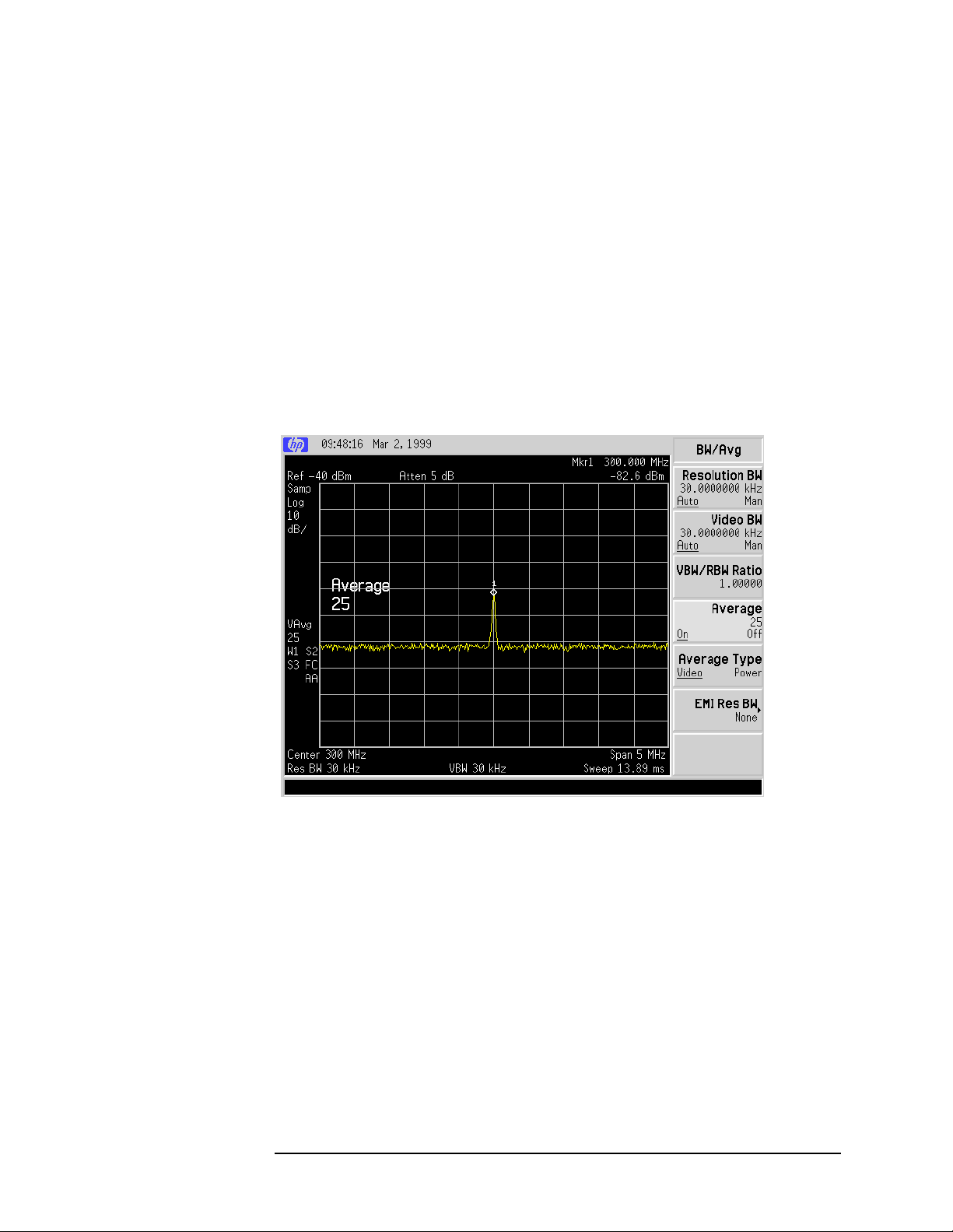
7. To set the number of samples, use the numbers keypad. Forexample, press

Average (On), 25, Enter. Turn video averaging off and on again

by pressing

Average (Off), Average (On). The number of samples

equals the number of sweeps in the averaging routine. During averaging, the current sample number appears at the left

side of the graticule. Changes in active functions settings, such as the center frequency or reference level, will restart the sampling. The sampling will also restart if video averaging is turned off and then on again.

Once the set number of sweeps has been completed, the analyzer continues to provide a running average based on this set number.

Figure 1-17 Using the Video Averaging Function

Making Basic Measurements

Measuring Low Level Signals

Chapter 1 1-27

Making Basic Measurements

Identifying Distortion Products

Distortion from the Analyzer

High level input signals may cause analyzer distortion products that could mask the real distortion measured on the input signal. Using trace 2 and the RF attenuator, you can determine which signals, if any, are internally generated distortion products.

Example:

Using a signal from a signal generator, determine whether the harmonic distortion products are generated by the analyzer.

1. As in the previous example, set the analyzer to view a low level signal. Connect a signal generator to the analyzer input. Press

Preset, Factory Preset (if displayed).

2. Connect a signal generator to the analyzer INPUT. Set the signal generator frequency to 200 MHz and the amplitude to 0 dBm.

3. Set the center frequency of the analyzer to 400 MHz and the span to 500 MHz by pressing FREQUENCY, 400 MHz, SPAN, 500 MHz. The signal shown in Figure 1-18 produces harmonic distortion products in the analyzer input mixer.

Figure 1-18 Harmonic Distortion

1-28 Chapter1

Making Basic Measurements

Identifying Distortion Products

4. Change the center frequency to the value of one of the observed harmonics.

5. Change the span to 50 MHz: press SPAN, 50 MHz.

6. Change the attenuation to 0 dB: press

0 dB.

7. To determine whether the harmonic distortion products are generated by the analyzer, ﬁrst save the screen data in trace 2.

Press

Write. Allow the trace to update (two sweeps) and press View, Peak Search, Marker, Delta. The analyzer display shows the stored data in

View/Trace, Trace 1 2 3 (until trace 2 is underlined), then Clear

trace 2 and the measured data in trace 1.

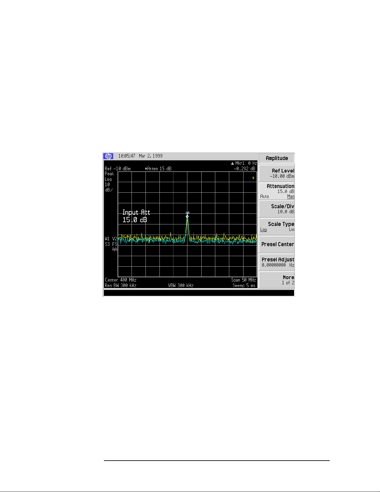
8. Next, increase the RF attenuation by 10 dB: press AMPLITUDE,

Attenuation , and the step-up key (↑) twice. See Figure 1-19.

Notice the ∆Mkr1 amplitude reading. This is the difference in the distortion product amplitude readings between 0 dB and 10 dB input attenuation settings. If the ∆Mkr1 amplitude reading is approximately >1 dB for an input attenuator change, the distortion is being generated, at least in part, by the analyzer. In this case more input attenuation is necessary.

Figure 1-19 RF Attenuation of 10 dB

AMPLITUDE, Attenuation (Man),

Chapter 1 1-29

Making Basic Measurements

Identifying Distortion Products

9. Press Peak Search, Meas Tools, Delta, then change the attenuation to 15 dB by pressing

Amplitude, Attenuation (Man), 15 dB.

If the ∆ Mkr1 amplitude reading is approximately >1 dB as seen in

Figure 1-19, then more input attenuation is required; some of the

measured distortion is internally generated. If there is no change in the signal level, the distortion is not generated internally. For example, the signal that is causing the distortion shown in Figure 1-20 is not high enough in amplitude to cause internal distortion in the analyzer so any distortion that is displayed is present on the input signal.

Figure 1-20 No Internally-Generated Harmonic Distortion

1-30 Chapter1

Making Basic Measurements

Identifying Distortion Products

Third-Order Intermodulation Distortion

Two-tone, third-order intermodulation distortion is a common test in communication systems. When two signals are present in a non-linear system, they can interact and create third-order intermodulation distortion products that are located close to the original signals. These distortion products are generated by system components such as ampliﬁers and mixers.

Example:

Test a device for third-order intermodulation. This example uses two sources, one set to 300 MHz and the other to approximately 301 MHz. (Other source frequencies may be substituted, but try to maintain a frequency separation of approximately 1 MHz.)

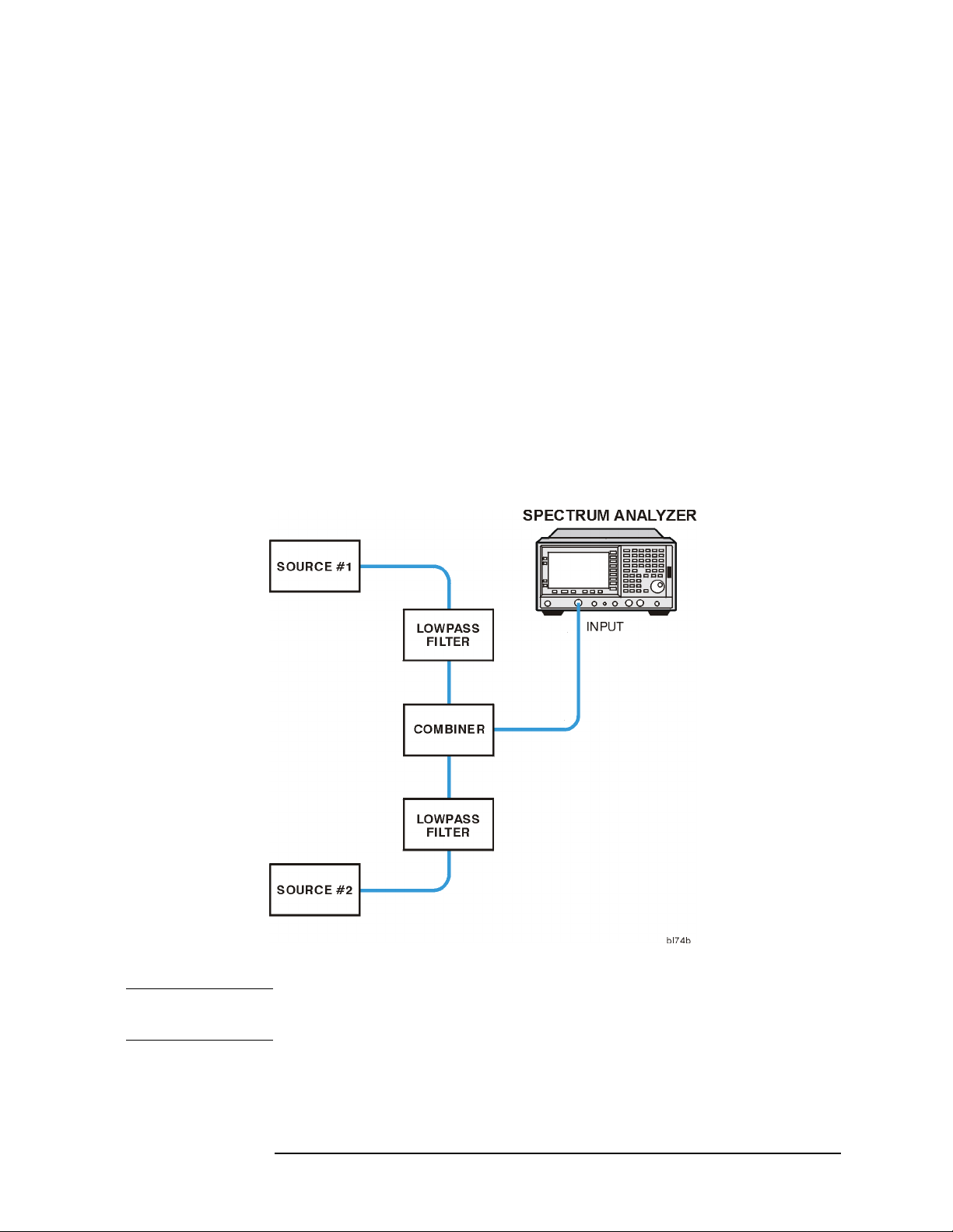
1. Connect the equipment as shown in Figure 1-21. Press

Factory Preset (if present).

Figure 1-21 Third-Order Intermodulation Equipment Setup

Preset,

NOTE The combiner should have a high degree of isolation between the two

input ports so the sources do not intermodulate.

Chapter 1 1-31

Making Basic Measurements

Identifying Distortion Products

2. Set one source to 300 MHz and the other source to 301 MHz, for a frequency separation of 1 MHz. Set the sources equal in amplitude (in this example, they are set to −5 dBm).

3. Tune both signals onto the screen by setting the center frequency

300.5 MHz. Then, using the knob, center the two signals on the display. Reduce the frequency span to 5 MHz. This is wide enough to include the distortion products on the screen. To be sure the distortion products are resolved, reduce the resolution bandwidth until the distortion products are visible.

4. For best dynamic range, set the mixer input level to −30 dBm and move the signal to the reference level: press

Mixer Lvl, 30 −dBm.

AMPLITUDE, More, Max

The analyzer automatically sets the attenuation so that a signal at the reference level will be a maximum of −30 dBm at the input mixer. Press

BW/Avg, Resolution BW, and then use the step-down key

(↓) to reduce the resolution bandwidth until the distortion products are visible.

5. To measure a distortion product, press on a source signal. To activate the second marker, press

Delta. Using the knob, adjust the second marker to the peak of the

Peak Search to place a marker

Marker,

distortion product that is beside the test signal. The difference between the markers is displayed in the active function area.

To measure the other distortion product, press

Peak. This places a marker on the next highest peak, which, in this

Peak Search, Next

case, is the other source signal. To measure the difference between this test signal and the second distortion product, press

Marker, Delta

and use the knob to adjust the second marker to the peak of the second distortion product. See Figure 1-22.

1-32 Chapter1

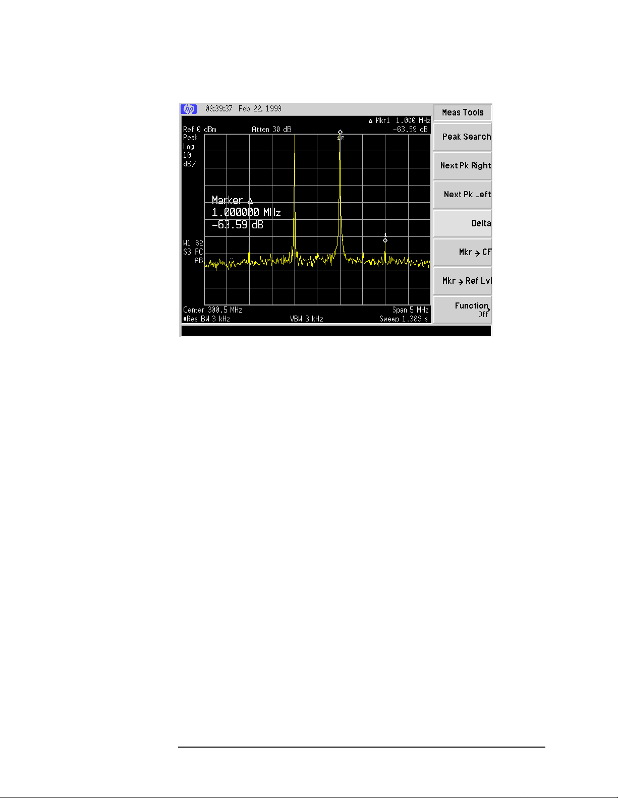
Figure 1-22 Measuring the Distortion Product

Making Basic Measurements

Identifying Distortion Products

See “Measuring Harmonics and Harmonic Distortion” on page 2-19 for more information about measuring distortion products.

Chapter 1 1-33

Making Basic Measurements

Measuring Signal-to-Noise

For this measurement the signal (carrier) is a discrete tone. If the signal is a carrier that is modulated under normal operation, you may use the amplitude reference signal as the signal of interest and the noise of the analyzer for the noise measurement. However, for this example, you will set the input attenuator such that both the signal and the noise are well within the calibrated region of the display. In this example the 50 MHz amplitude reference signal is used as the fundamental source.

Perform the steps below to measure the signal-to-noise.

1. Turn on the 50 MHz amplitude reference signal of the analyzer (if you have not already done so).

For the E4401B and E4411B, use the 50 MHz amplitude reference signal of the analyzer as the signal being measured. Press

Factory Preset (if present), Input/Output, Amptd Ref (On).

Preset,

Forall other models connect a cable between the front-panel AMPTD REF OUT to the analyzer INPUT, then press Preset, Factory Preset (if present), Input/Output, Amptd Ref Out (On).

2. Set the center frequency to 50 MHz and the span to 1 MHz: press

FREQUENCY, 50 MHz, SPAN, 1 MHz.

3. Set the reference level to −10 dBm by pressing

−10 dBm.

4. Set the attenuation to 40 dB by pressing

40 dB.

5. Press

6. Press

Peak Search to place a marker on the peak of the signal. Marker, Delta, 200 kHz to put the delta marker in the noise at

AMPLITUDE, Ref Level,

AMPLITUDE, Attenuation,

the speciﬁed offset, in this case 200 kHz.

7. Press More 1 of 2, Function, Marker Noise to view the results of the signal to noise measurement. See Figure 1-23.

1-34 Chapter1

Figure 1-23 Measuring the Signal-to-Noise

Making Basic Measurements

Measuring Signal-to-Noise

Read the signal-to-noise in dB/Hz, that is with the noise value determined for a 1-Hz noise bandwidth. If you wish the noise value for a different bandwidth, decrease the ratio by . For example, if

10 log× BW()

the analyzer reading is −70 dB/Hz but you have a channel bandwidth of 30 kHz:

S/N 70 dB/Hz– 10 log 30 kHz()25.2 dB/30 kHz–=×+=

Note that the display detection mode is now sample. If the delta marker is within half a division of the response to a discrete signal, the amplitude reference signal in this case, there is a potential for error in the noise measurement. See “Making Noise Measurements” on page 36.

Chapter 1 1-35

Making Basic Measurements

Making Noise Measurements

There are a variety of ways to measure noise power. The ﬁrst decision you must make is whether you want to measure noise power at a speciﬁc frequency or the total power over a speciﬁed frequency range, for example over a channel bandwidth.

Example 1:

Using the marker function, Marker Noise, is a simple method to make a measurement at a single frequency. In this example, attention must be made to the potential errors due to discrete signal (spectral components). This measurement will be made near the 50 MHz amplitude reference signal to illustrate the use of

1. Turn on the 50 MHz amplitude reference signal of the analyzer (if you have not already done so).

For the E4401B and E4411B, use the 50 MHz amplitude reference signal of the analyzer as the signal being measured. Press

Factory Preset (if present), Input/Output, Amptd Ref (On).

Marker Noise.

Preset,

Forall other models connect a cable between the front-panel AMPTD REF OUT to the analyzer INPUT, then press

Preset, Factory Preset

(if present), Input/output, Amptd Ref Out (On).

2. Tune the analyzer to the frequency of interest. In this example we are using the reference signal. Press FREQUENCY, 49.98 MHz.

3. Set the span to 100 kHz by pressing

4. Set the reference level to −20 dBm by pressing

−20 dBm. See Figure1-24. Note that if the signal is much higher than

SPAN, 100 kHz.

AMPLITUDE, Ref Level,

shown, adjust the input attenuator. In this example the input attenuation was set to 60 dB by pressing

Attenuation, 60 dB.

1-36 Chapter1

Figure 1-24 Setting the Reference Level

Making Basic Measurements

Making Noise Measurements

5. Activate the noise marker by pressing

Marker Noise.

Note that the display detection has changed to sample, the marker ﬂoats between the maximum and the minimum of the noise. The marker readout is in dBm(Hz) or dBm per unit bandwidth. See

Figure 1-25. For noise power in a different bandwidth, add

10 log× BW() 10 log 1000()×

. For example, for noise power in a 1 kHz bandwidth, add

or 30 dB to the noise marker value.

Figure 1-25 Activating the Noise Marker

Marker, More 1 of 2, Function,

Chapter 1 1-37

Making Basic Measurements

Making Noise Measurements

6. Video ﬁltering can be introduced to reduce the variations of the sweep-to-sweep marker value. Set the video ﬁlter by pressing

BW/Avg, Video BW (Man), 100 Hz.

Notice that these variations are to be expected due to the nature of the signal. We can reduce the variations by introducing video ﬁltering. Since reducing the video bandwidth ﬁlter impacts sweep time, it is recommended to limit the degree of ﬁltering.

7. The noise marker value is based on the mean of 33 trace points centered at the marker. With a total of 401 points across the entire trace, the 33 points span almost a full division. To see the effect, move the marker to the 50 MHz signal by pressing

Marker, 50 MHz (or

use the knob to place marker at 50 MHz).

8. The marker does not go to the peak of the signal because not all 33 points are at the peak of the signal. Widen the resolution bandwidth by pressing

BW/Avg, Resolution BW (Man),10 kHz (or up arrow) to see

what happens. The marker is now much closer to the peak of the signal.

9. Return the resolution bandwidth to automatic mode by pressing

Resolution BW (Auto).

10. Measure the noise very close to the signal by pressing

49.99625 MHz (or use the knob to place the marker).

Marker,

Note that the marker reads a value that is too high because some of the 33 trace points are on the skirt of the signal response.

11. Set the analyzer for zero span by pressing

SPAN, Zero Span, Marker.

Note that the marker value is now correct.

Example 2:

The Normal marker can also be used to make a single frequency measurement as described in the previous example, again using video ﬁltering or averaging to obtain a reasonably stable measurement. While video averaging automatically selects the sample display detection mode, video ﬁltering does not. With sufﬁcient ﬁltering that results in a smooth trace, there is no difference between the sample and peak modes because the ﬁltering takes place before the signal is digitized.

Be sure to account for the fact that the averaged noise is displayed approximately 2 dB too low for a noise bandwidth equal to the resolution bandwidth. Therefore, you must add 2 dB to the marker reading. For example, if the marker indicates −100 dBm, the actual noise level is −98 dBm.

1-38 Chapter1

Making Basic Measurements

Making Noise Measurements

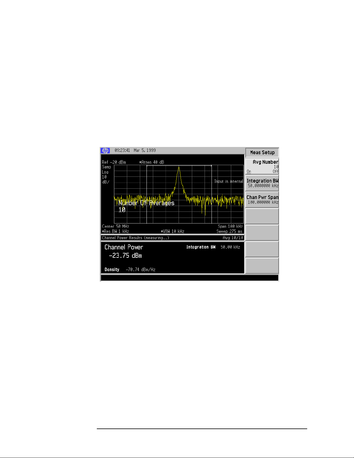
Example 3:

You may want to measure the total power of a noise-like signal that occupies some bandwidth. Forexample, you may want to determine the power in a communications channel. If the signal is noise and is ﬂat across the band of interest, you can use the noise marker as described in example 1 and add . However, if you are not certain of the characteristics of the signal, or if there are discrete spectral components in the band of interest, we can use the Channel Power routine. In this example,you will use the noise of the analyzer, then add a discrete tone to see what happens and assume a channel bandwidth of 50 kHz. If desired, a speciﬁc signal may be substituted.

10 log channel BW()×

1. Reset the analyzer by pressing

Preset, Factory Preset (if present).

2. Tune the analyzer to the frequency of 50 MHz. In this example we are using the amplitude reference signal. Press FREQUENCY, 50 MHz.

3. Set the span to 100 kHz by pressing

4. Set the reference level to −20 dBm by pressing

−20 dBm.

5. Set the input attenuation to 40 dB by pressing

SPAN, 100 kHz.

AMPLITUDE, Ref Level,

Attenuation, 40 dB.

6. Set the analyzer to setup the channel-power measurement by pressing MEASURE, Channel Power, Meas Setup.

7. Set the integration bandwidth to 50 kHz by pressing

50 kHz.

8. Set the channel-power span to 100 kHz by pressing

100 kHz.

NOTE The display detection mode has been set to sample and the video

Integration BW,

Chan Pwr Span,

bandwidth has been set to be ten times wider than the resolution bandwidth. This setting is important to prevent any averaging.Youcan reduce the sweep-to-sweep variation in the power reading by averaging over a number of sweeps.

9. Turn average number on by pressing

Avg Number (On). 10 is an

acceptable number.

Chapter 1 1-39

Making Basic Measurements

Making Noise Measurements

10.Add a discrete tone to see the affects of the reading. Turn on the 50 MHz amplitude reference signal of the analyzer (if you have not already done so).

For the E4401B and E4411B, use the 50 MHz amplitude reference signal of the analyzer as the signal being measured. Press

Input/Output, Amptd Ref (On).

Forall other models connect a cable between the front-panel AMPTD REF OUT to the analyzer INPUT, then press Input/Output, Amptd Ref

Out (On). Your display should be similar to Figure 1-26.

Figure 1-26 Measuring Channel Power

The power reading is essentially that of the tone; that is, the total noise power is far enough below that of the tone that the noise power contributes very little to the total.

The algorithm that computes the total power compensates for the fact that some of the trace points on the response to the continuous wave tone may be at or very close to the peak value of the tone and so yields the correct value whether the signal comprises just noise, a tone, or both.

1-40 Chapter1

Making Basic Measurements

Making Noise Measurements

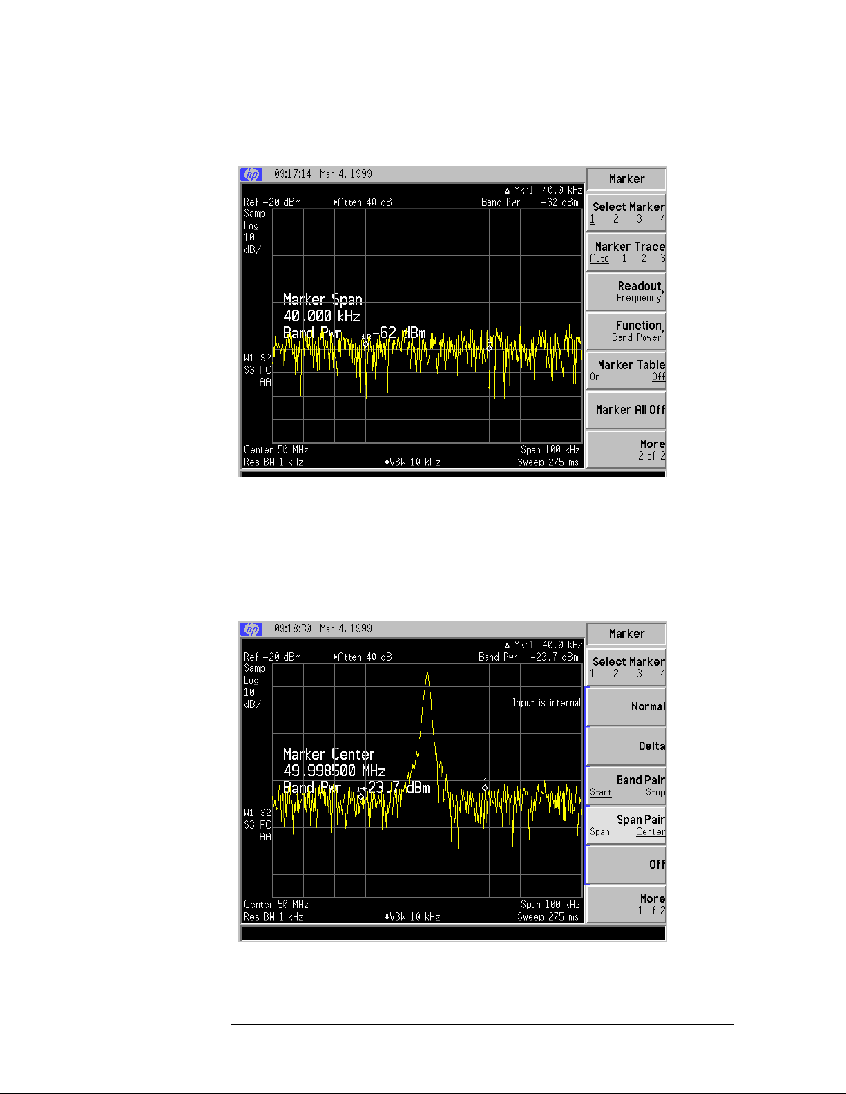
Example 4:

The functions described in example 3 also allow you to measure the total power of noise-like signals, tones, or both. A difference is that you use adjustable markers to set the frequency span over which power is measured. The markers allow you to easily and conveniently select any arbitrary portion of the displayed signal for measurement. However, while the analyzer does select the sample display detection mode, you must set all of the other parameters.

1. Reset the analyzer by pressing

Preset, Factory Preset (if present).

2. Tune the analyzer to the frequency of 50 MHz. In this example we are using the amplitude reference signal. Press FREQUENCY, 50 MHz.

3. Set the span to 100 kHz by pressing

4. Set the reference level to −50 dBm by pressing

−20 dBm.

5. Set the input attenuator to 40 dB by pressing

6. Set the marker span to 40 kHz by pressing

40 kHz.

SPAN, 100 kHz.

AMPLITUDE, Ref Level,

Attenuation, 40 dB.

Marker, Span Pair (Span),

The resolution bandwidth should be about 1 to 3% of the measurement (marker) span, 40 kHz in this example. The 1 kHz resolution bandwidth that the analyzer has chosen is ﬁne. The video bandwidth should be ten times wider.

7. Set the video bandwidth to 10 kHz by pressing

(Man),10 kHz.

8. Measure the power between markers by pressing

Function, Band Power.The analyzer displays the total power between

BW/Avg, Video BW

Marker, More 1 of 2,

the markers. See Figure 1-27.

9. Add a discrete tone to see the affects of the reading. Turn on the 50 MHz amplitude reference signal of the analyzer (if you have not already done so).

For the E4401B and E4411B, use the 50 MHz amplitude reference signal of the analyzer as the signal being measured. Press

Input/Output, Amptd Ref (On).

Forall other models connect a cable between the front-panel AMPTD REF OUT to the analyzer INPUT, then press Input/Output, Amptd Ref

Out (On).

Chapter 1 1-41

Making Basic Measurements

Making Noise Measurements

Figure 1-27 Viewing Power Between Markers

10.Move the measured span by pressing use the knob to exclude the tone and note reading. You could have also used

Band Pair to set the measurement start and stop points

independently. See Figure 1-28.

Figure 1-28 Measuring the Power of the Span

Marker, Span Pair(Center). Then

1-42 Chapter1

Making Basic Measurements

Demodulating AM Signals (Using the Analyzer As a Fixed Tuned Receiver)

The zero span mode can be used to recover amplitude modulation on a carrier signal. The analyzer operates as a ﬁxed-tuned receiver in zero span to provide time domain measurements.

Center frequency in the swept-tuned mode becomes the tuned frequency in zero span. The horizontal axis of the screen becomes calibrated in time only, rather than both frequency and time. Markers display amplitude and time values.

The following functions establish a clear display of the waveform:

• Trigger stabilizes the waveform trace on the display by triggering on the modulation envelope. If the modulation of the signal is stable, video trigger synchronizes the sweep with the demodulated waveform.

• Linear mode should be used in amplitude modulation (AM) measurements to avoid distortion caused by the logarithmic ampliﬁer when demodulating signals.

• Sweep time adjusts the full sweep time from 5 ms to 2000 s. (20 us to 2000 s if Option AYX is installed). The sweep time readout refers to the full 10-division graticule. Divide this value by 10 to determine sweep time per division.

• Resolution and video bandwidth are selected according to the signal bandwidth.

Each of the coupled function values remains at its current value when zero span is activated. Video bandwidth is coupled to resolution bandwidth. Sweep time is not coupled to any other function.

NOTE Refer to “Demodulating and Listening to an AM Signal” on page 2-15

for more information on signal demodulation.

Example:

View the modulation waveform of an AM signal in the time domain.

1. Connect an RF signal source to the analyzer INPUT. For this example, an HP/Agilent ESG-4000A Signal Generator (Model E4422A) was used with the following settings:

RF Frequency 300 MHz, RF Output Power –10 dBm, AM On, AM Rate 1 kHz AM Depth 80%

2. Preset the analyzer by pressing

Chapter 1 1-43

Preset, Factory Preset (if present).

Making Basic Measurements

Demodulating AM Signals (Using the Analyzer As a Fixed Tuned Receiver)

3. Set the center frequency of the analyzer to 300 MHz by pressing

FREQUENCY, 300 MHz.

4. Set the Span to 500 kHz by pressing adjust the analyzer center frequency to center the signal horizontally on the display by pressing rotating the knob.

5. Set the resolution bandwidth to 30 kHz by pressing BW/Avg,

Resolution BW, 30 kHz. This setting is wide enough to include both

1 kHz AM sidebands of the RF carrier well within the 1 dB passband of the analyzer.

6. Change the analyzer sweep to 20 ms by pressing

20 ms. The 1 kHz amplitude modulation is now clearly visible as

amplitude variations of the trace with 1 ms peak-to-peak spacing. See Figure 1-29.

Figure 1-29 Viewing an AM Signal

SPAN, 500 kHz. If necessary,

FREQUENCY, Center Freq, and

Sweep, Sweep Time,

7. Position the signal peak near the reference level by pressing

AMPLITUDE and rotating the knob.

8. Change the amplitude scale type to linear by pressing

Scale Type (Lin).

1-44 Chapter1

AMPLITUDE,

Demodulating AM Signals (Using the Analyzer As a Fixed Tuned Receiver)

9. To select zero span, press either SPAN, 0 Hz, or SPAN, Zero Span. Change the sweep time to 5 ms by pressing

5ms. See Figure 1-30. Since the modulation is a steady tone, you can

use video trigger to trigger the analyzer sweep on the waveform and stabilize the trace, much like an oscilloscope (press adjust the trigger level with the knob).

Use markers and delta markers to measure the time parameters of the waveform. Adjust the sweep time to change the horizontal scale. Adjust the reference level to change the vertical scale.

Figure 1-30 Measuring Modulation In Zero Span

Making Basic Measurements

Sweep, Sweep Time (Man),

Trig, Video, and

Chapter 1 1-45

Making Basic Measurements

Demodulating FM Signals (Without Option BAA)

As with amplitude modulation (see page 1-43) you can utilize zero span to demodulate an FM signal. However, unlike the AM case, you cannot simply tune to the carrier frequency and widen the resolution bandwidth. The reason is that the envelope detector in the analyzer responds only to amplitude variations, and there is no change in amplitude if the frequency changes of the FM signal are limited to the ﬂat part of the resolution bandwidth.

On the other hand, if you tune the analyzer slightly away from the carrier, you can utilize slope detection to demodulate the signal by performing the following steps.

1. Determine the correct resolution bandwidth.

2. Find the center of the linear portion of the ﬁlter skirt (either side).

3. Tune the analyzer to put the center point at mid screen of the display.

4. Select zero span.

The demodulated signal is now displayed; the frequency changes have been translated into amplitude changes. To listen to the signal, turn on AM demodulation and the speaker.

In this example you will demodulate a broadcast FM signal that has a speciﬁed 75 kHz peak deviation.

Example:

Determine the correct resolution bandwidth. With a peak deviation of 75 kHz, your signal has a peak-to-peak excursion of 150 kHz. So we must ﬁnd a resolution bandwidth ﬁlter with a skirt that is reasonably linear over that frequency range.

1. Turn on the 50 MHz amplitude reference signal of the analyzer (if you have not already done so).

For the E4401B and E4411B, use the 50 MHz amplitude reference signal of the analyzer as the signal being measured. Press

Factory Preset (if present), Input/Output, Amptd Ref (On).

Preset,

Forall other models connect a cable between the front-panel AMPTD REF OUT to the analyzer INPUT, then press Preset, Factory Preset (if present), Input/Output, Amptd Ref Out (On).

1-46 Chapter1

Making Basic Measurements

Demodulating FM Signals (Without Option BAA)

2. Tune the analyzer to the frequency of 50 MHz. In this example we are using the amplitude reference signal. Press

FREQUENCY, 50 MHz.

3. Set the span to 1 MHz by pressing

4. Set the reference level to −20 dBm by pressing

−20 dBm.

5. Set the resolution bandwidth to 100 kHz by pressing

Resolution BW, 100 kHz. The skirt is reasonably linear starting about

half a division down from the peak.

6. Select a marker by pressing Marker, then move the marker approximately one division down the right of the peak (high frequency) using the front-panel knob.

7. Place a delta marker 150 kHz from the ﬁrst marker by pressing

Delta, 150 kHz. The skirt looks reasonably linear between markers.

8. Determine the offset from the signal peak to the desired point on the ﬁlter skirt by moving the delta marker to the midpoint. Press 75 kHz to move the delta marker to the midpoint. See Figure 1-31.

Figure 1-31 Determining the Offset

SPAN, 1 MHz.

AMPLITUDE, Ref Level,

BW/Avg,

9. Press

10.Press

Delta to make the active marker the reference marker. Search to move the delta marker to the peak. The delta value

is the desired offset, for example 140 kHz.

Chapter 1 1-47

Making Basic Measurements

Demodulating FM Signals (Without Option BAA)

Demodulate the FM Signal

1. Connect an antenna to the analyzer INPUT.

2. Reset the analyzer by pressing

Preset, Factory Preset (if present).

3. Tune the analyzer to the peak of one of your local FM broadcast signals, for example 97.7 MHz by pressing FREQUENCY, 97.7 MHz.

4. Tune above or below the FM signal by the offset noted above in step 11, in this example 140 kHz. Press FREQUENCY, CF Step 140 kHz, then use the step-up key (↑) or step-down key (↓).

5. Set the resolution bandwidth to 100 kHz, then go to zero span by pressing

6. Turn off the automatic alignment by pressing

Auto Align, Off.

7. Activate single sweep by pressing

BW/Avg, Resolution BW, 100 kHz, SPAN, Zero Span.

System, Alignments,

Single.

8. Listen to the demodulated signal through the speaker by pressing

Det/Demod, Demod, AM, Return, Speaker (On), then adjust the volume

using the front-panel volume knob.

1-48 Chapter1

2 Making Measurements

2-1

Making Measurements

What’s in This Chapter

This chapter provides information for making complex measurements. The procedures covered in this chapter are listed below.

• “Making Stimulus Response Measurements” on page 2-3

• “Making a Reﬂection Calibration Measurement” on page 2-12

• “Demodulating and Listening to an AM Signal” on page 2-15

• “Measuring Harmonics and Harmonic Distortion” on page 2-19

• “Demodulating and Viewing Television Signals (Option B7B)” on

page 2-25

• “Using External Millimeter Mixers (Option AYZ)” on page 2-33

To ﬁnd descriptions of speciﬁc analyzer functions refer to the user’s guide for your instrument.

2-2 Chapter2

Making Measurements

Making Stimulus Response Measurements

What Are Stimulus Response Measurements?

Stimulus response measurements require asource to stimulate a device under test (DUT), a receiver to analyze the frequency response characteristics of the DUT, and, for return loss measurements, a directional coupler or bridge. Characterization of a DUT can be made in terms of its transmission or reﬂection parameters. Examples of transmission measurements include ﬂatness and rejection. Return loss is an example of a reﬂection measurement.

A spectrum analyzer combined with a tracking generator forms a stimulus response measurement system. With the tracking generator as the swept source and the analyzer as the receiver, operation is the same as a single channel scalar network analyzer. The tracking generator output frequency must be made to precisely track the analyzer input frequency for good narrow band operation. A narrow band system has a wide dynamic measurement range. This wide dynamic range will be illustrated in the following example.

Using An Analyzer With A Tracking Generator

There are three basic steps in performing a stimulus response measurement, whether it is a transmission or a reﬂection measurement. The steps are to set all the analyzer settings, normalize, and measure.

The procedure below describes how to use a built in tracking generator system to measure the rejection of a bandpass ﬁlter, a type of transmission measurement. Illustrated in this example are functions in the tracking generator menu such as adjusting the tracking generator output power. Normalization functions located in the trace menu are also used. Making a reﬂection measurement is similar and is covered in

“Making a Reﬂection Calibration Measurement” on page 2-12.

Chapter 2 2-3

Making Measurements

Making Stimulus Response Measurements

Stepping Through a Transmission Measurement

1. To measure the rejection of a bandpass ﬁlter, connect the equipment as shown in Figure 2-2. This example uses a 177 MHz bandpass ﬁlter.

Figure 2-1 Transmission Measurement Test Setup

2. Access the tracking generator functionality using the source key on the analyzer. To activate the tracking generator power level, press

Source, Amplitude (On). See Figure 2-2.

CAUTION Excessive signal input may damage the DUT. Do not exceed the

maximum power that the device under test can tolerate.

NOTE To reduce ripples caused by source return loss, use 10 dB (E4401B or

E4411B) or 8 dB (all other models) or greater tracking generator output attenuation. Tracking generator output attenuation is normally a function of the source power selected. However, the output attenuation may be controlled in the

Source menu. Refer to speciﬁcations and

characteristics in your user’s and calibration guide for more information on the relationship between source power and source attenuation.

2-4 Chapter2

Making Stimulus Response Measurements

Figure 2-2 Tracking Generator Output Power Activated

Making Measurements

3. Put the sweep time of the analyzer into stimulus response auto coupled mode by pressing

Sweep, then Swp Coupling (SR) (for

stimulus response mode). Auto coupled sweep times are usually much faster for stimulus response measurements than they are for spectrum analyzer (SA) measurements. Adjust the reference level if necessary to place the signal on screen.

NOTE In the stimulus response mode, the Q of the DUT can determine the

fastest rate at which the analyzer can be swept. (Q is the quality factor, which is reactance versus resistance.) To determine whether the analyzer is sweeping too fast, slow the sweep and note whether there is a frequency or amplitude shift of the trace. Continue to slow the sweep until there is no longer a frequency or amplitude shift.

Since we are only interested in the rejection of the bandpass ﬁlter ±125 MHz from the center of the bandpass, tune the analyzer center frequency and span to center the bandpass response and display the rejection ±150 MHz from the center of the bandpass.

Chapter 2 2-5

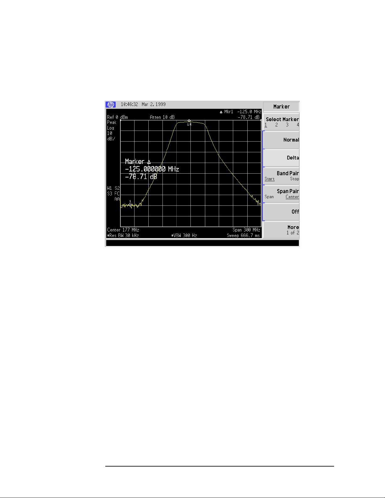
Making Measurements

Making Stimulus Response Measurements

4. Decrease the resolution bandwidth to increase sensitivity, and narrow the video bandwidth to smooth the noise. In Figure 2-3, the resolution bandwidth has been decreased to 30 kHz.

Figure 2-3 Decrease the Resolution Bandwidth to Improve Sensitivity

5. You might notice a decrease in the displayed amplitude as the resolution bandwidth is decreased, (if the analyzer is an E4402B, E4403B, E4404B, E4405B, E4407B, or E4408B). This indicates the need for performing a tracking peak. Press

Source, Tracking Peak.

The amplitude should return to that which was displayed prior to the decrease in resolution bandwidth.

6. To make a transmission measurement accurately, the frequency response of the test system must be known. Normalization is then used to eliminate this error from the measurement. To measure the frequency response of the test system, connect the cable (but not the DUT) from the tracking generator output to the analyzer input. Press

Normalize (On). The frequency response of the test system is now

View/Trace, More 1 of 2, Normalize, Store Ref (if present),

stored in normalize trace and a normalization is performed. This means that the active displayed trace is now the ratio of the input data to the data stored in the normalized trace (Trace 3 with ﬁrmware revision A.04.00 and later).

When normalization is on, trace math is being performed on the active trace. The trace math performed is (trace 1 − normalized trace + the normalized reference position), with the result placed into trace 1. Remember that trace 1 contains the measurement trace, normalized trace contains the stored calibration trace of the system

2-6 Chapter2

Making Measurements

Making Stimulus Response Measurements

frequency response, and normalized reference position is indicated by arrowheads at the edges of the graticule.

7. Reconnect the DUT to the analyzer. Note that the units of the reference level have changed to dB, indicating that this is now a relative measurement. Press

Norm Ref Posn to change the

normalized reference position. Arrowheads at the left and right edges of the graticule mark the normalized reference position, or the position where 0 dB insertion loss (transmission measurements) or 0 dB return loss (reﬂection measurements) will normally reside. Using the knob results in a change in the position of the normalized trace, within the range of the graticule.

8. To measure the rejection of the ﬁlter 125 MHz below the center of the bandpass, press

Peak Search, Marker, Delta, −125 MHz, and enter

the frequency. The marker readout displays the rejection of the ﬁlter at 125 MHz. See Figure 2-4.

NOTE Because the default number of sweep points per trace is 401, the

indicated marker frequency may differ slightly from the frequency that you entered. Due to the horizontal resolution of the trace, the marker frequency value will be rounded to within 0.25% of the span of the value entered. If the analyzer is an ESA-E series with ﬁrmware revision A.04.00 or later, the number of sweep points may be set to any value between 101 and 8192.

Figure 2-4 Measure the Rejection Range

Chapter 2 2-7

Making Measurements

Making Stimulus Response Measurements

Tracking Generator Unleveled Condition

When using the tracking generator, the message TG unleveled may appear. The TG unleveled message indicates that the tracking generator source power ( maintained at the selected level during some portion of the sweep. If the unleveled condition exists at the beginning of the sweep, the message will be displayed immediately. If the unleveled condition occurs after the sweep begins, the message will be displayed after the sweep is completed. A momentary unleveled condition may not be detected when the sweep time is short. The message will be cleared after a sweep is completed with no unleveled conditions.

The unleveled condition may be caused by any of the following:

• Start frequency is too low or the stop frequency is too high. The unleveled condition is likely to occur if the true frequency range exceeds the tracking generator frequency speciﬁcation (especially the low frequency speciﬁcation).

• Source attenuation may be set incorrectly (select for optimum setting).

• The source power may be set too high or too low, use reset it.

• The source power sweep may be set too high, resulting in an unleveled condition at the end of the sweep. Use decrease the amplitude.

• Reverse RF power from the device under test detected by the tracking generator ALC (automatic level control) system.

Source, Amplitude On Off) could not be

Attenuation (Auto)

Amplitude to

Power Sweep to

2-8 Chapter2

Making Measurements

Making Stimulus Response Measurements

Measuring Device Bandwidth

It is often necessary to measure device bandwidth, such as when testing a bandpass ﬁlter. There is a key in the perform this function. The device signal being measured must be displayed before activating the measurement. The span must include the full response.

Peak Search menu that will

Activate the measurement by pressing places arrow markers at the −3 dB points on either side of the response and reads the bandwidth. For other bandwidth responses enter the number of dB down desired, from −1 dB to −80 dB.

No other signal can appear on the display within N dB of the highest signal. The measured signal cannot have more than one peak that is greater than or equal to N dB. A signal must have a peak greater than the currently deﬁned peak excursion to be identiﬁed. The default value for the peak excursion is 6 dB.

Measurements are made continuously, updating at the end of each sweep. This allows you to make adjustments and see changes as they happen. The single sweep mode can also be used, providing time to study or record the data.

The N dB bandwidth measurement error is typically ±1% of the span.

Figure 2-5 N dB Bandwidth Measurement

N dB Points (On). The analyzer

Chapter 2 2-9

Making Measurements

Making Stimulus Response Measurements

Example:

Measure the 3 dB bandwidth of a 177 MHz bandpass ﬁlter.

1. To measure the rejection of a bandpass ﬁlter, connect the equipment as shown in Figure 2-6. This example uses a 177 MHz bandpass ﬁlter.

Figure 2-6 Transmission Measurement Test Setup

2. Access the tracking generator functionality using the source key on the analyzer. To activate the tracking generator power level, press

Source, Amplitude (On). See Figure 2-2.

CAUTION Excessive signal input may damage the DUT. Do not exceed the

maximum power that the device under test can tolerate.

NOTE To reduce ripples caused by source return loss, use 10 dB (E4401B or

Source menu. Refer to speciﬁcations and

characteristics in your user’s and calibration guide for more information on the relationship between source power and source attenuation.

2-10 Chapter2

Making Stimulus Response Measurements

Figure 2-7 Tracking Generator Output Power Activated

Making Measurements

3. Put the sweep time of the analyzer into stimulus response auto coupled mode by pressing

Sweep, then Swp Coupling SR SA until SR

(stimulus response mode) is underlined. Auto coupled sweep times are usually much faster for stimulus response measurements than they are for spectrum analyzer (SA) measurements. Adjust the reference level if necessary to place the signal on screen.

NOTE In the stimulus response mode, the Q of the DUT can determine the

4. Press

Peak Search, More 1 of 2, then N dB Points (On) to activate the

N dB bandwidth function.

5. Read the measurement results displayed on the screen.

6. The knob or the data entry keys can be used to change the N dB value from −3 dB to −60 dB to measure the 60 dB bandwidth of the ﬁlter.

7. Press

N dB Points (Off) to turn the measurement off.

Chapter 2 2-11

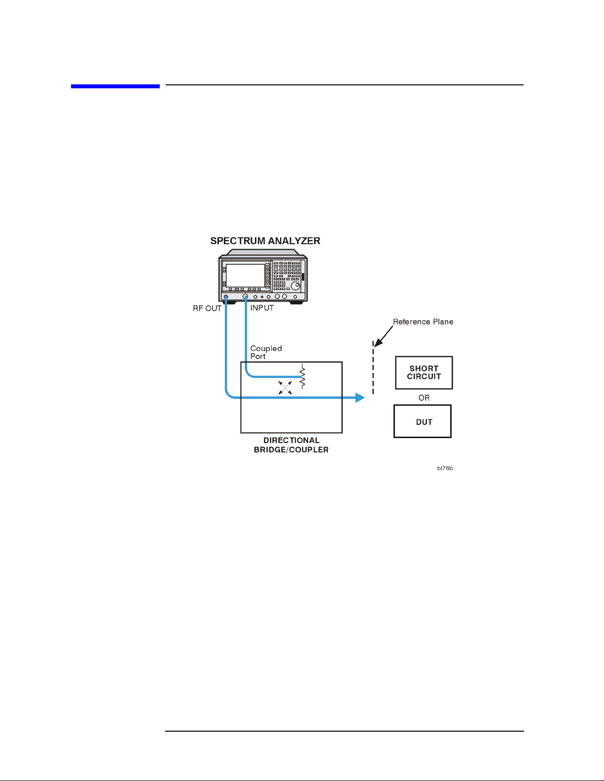
Making Measurements

Making a Reﬂection Calibration Measurement

The calibration standard for reﬂection measurements is usually a short circuit connected at the reference plane (the point at which the test device will be connected.) See Figure 2-8. A short circuit has a reﬂection coefﬁcient of 1 (0 dB return loss). It reﬂects all incident power and provides a convenient 0 dB reference.

Figure 2-8 Reﬂection Measurement Short Calibration Test Setup

2-12 Chapter2

Making Measurements

Making a Reﬂection Calibration Measurement

Example:

Measure the return loss of a ﬁlter. The following procedure makes a reﬂection measurement using a coupler or directional bridge.

Reﬂection Calibration

NOTE The analyzer center frequency and span for this measurement can

easily be set up using the transmission measurement setup in “Making

Stimulus Response Measurements” on page 2-3. Tune the analyzer so

that the passband of the ﬁlter comprises a majority of the display, then proceed with the steps outlined below.

1. Connect the DUT to the directional bridge or coupler as shown in

Figure 2-8. Terminate the unconnected port of the DUT.

NOTE If possible, use a coupler or bridge with the correct test port connector

for both calibrating and measuring. Any adapter between the test port and DUT degrades coupler/bridge directivity and system source match. Ideally, you should use the same adapter for the calibration and the measurement. Be sure to terminate the second port of a two port device.

2. Connect the tracking generator output of the analyzer to the directional bridge or coupler.

3. Connect the analyzer input to the coupled port of a directional bridge or coupler.

4. Set center frequency, span, and other analyzer settings. Turn on the tracking generator and set the amplitude level by pressing

Amplitude (On).

Source,

5. Replace the DUT with a short circuit.

6. Normalize the trace by pressing

Store Ref (if present). Then press Normalize (On), to activate the trace

View/Trace, More 1 of 2, Normalize,

1 minus normalized trace function and display the results in trace 1. The normalized trace or ﬂat line represents 0 dB return loss. Normalization occurs each sweep. Replace the short circuit with the DUT.

Chapter 2 2-13

Making Measurements

Making a Reﬂection Calibration Measurement

Measuring the Return Loss

1. After calibrating the system with the above procedure, reconnect the ﬁlter in place of the short circuit without changing any analyzer settings.

2. Use the marker to read return loss. Press marker with the knob to read the return loss at that frequency. Or you can use the pressing

Peak Search, Min Search, the analyzer will place a marker at

Min Search function to measure return loss by

the point where the return loss is maximized. See Figure 2-9.

Figure 2-9 Measuring the Return Loss of the Filter

Marker and position the

2-14 Chapter2

Making Measurements

Demodulating and Listening to an AM Signal

The functions listed in the menu under Det/Demod allow you to demodulate and hear signal information displayed on the analyzer. Simply place a marker on a signal of interest, activate AM demodulation, turn the speaker on, and then listen.

Example 1:

1. Connect an antenna to the analyzer input.

2. Select a frequency range on the analyzer, such as the range for AM radio broadcasts. For example, the frequency range for AM broadcasts in the United States is 550 kHz to 1650 kHz. Press

Preset, Factory Preset (if present), FREQUENCY, Start Freq, 550 kHz, Stop Freq, 1650 kHz.

3. Place a marker on the signal of interest by pressing place a marker on the highest amplitude signal, or by pressing

Marker, Normal and moving the marker to a signal of interest.

4. Press

Det/Demod, Demod, AM. Use the front-panel volume knob to

control the speaker volume.

Figure 2-10 Demodulation of an AM Signal

Peak Search to

Chapter 2 2-15

Making Measurements

Demodulating and Listening to an AM Signal

5. The signal is demodulated at the marker position only for the duration of the demod time. Use the step keys, knob, or numbers keypad to change the demod time. For example, press the step up key (↑) to increase the demod time to 2 seconds.

6. The marker search functions can be used to move the marker to other signals of interest. Press

Pk Right, or Next Pk Left.

NOTE Prior to each occurrence of the AM Demod Time period, the analyzer

Peak Search to access Next Peak, Next

automatically adjusts the marker level to the reference level, tunes the analyzer center frequency to the marker frequency (zero span) and sets the resolution bandwidth and video bandwidth to 30 kHz. The original analyzer settings are restored prior to each sweep.

2-16 Chapter2

Making Measurements

Demodulating and Listening to an AM Signal

Example 2:

1. Place the marker on a signal of interest as in steps 1 through 3 of the previous example.

2. If the signal of interest is the highest amplitude on screen signal, set the frequency of the signal to center frequency by pressing

FREQUENCY then Signal Track (On). If it is not the highest amplitude

signal on screen, move the signal to center screen by pressing

Peak Search and Mkr→CF.

3. If signal track function is on, press

SPAN and 1 MHz to reduce the

span to 1 MHz. If signal track is not used, use the step down key (↓) to reduce the span and use

Mkr→CF to keep the signal of interest at

center screen.

4. Set the span to zero by pressing SPAN, Zero Span. Zero Span turns off the signal track function.

5. Change the resolution bandwidth to 100 kHz by pressing BW/Avg,

Resolution BW (Man), then enter 100 kHz.

6. Set the signal in the top two divisions of the screen by changing the reference level. Press AMPLITUDE, and then the step down key (↓) until the signal is in the top two divisions. Set the amplitude scale to linear by pressing

7. Press

Det/Demod, Detector, Sample to set the detector mode of the

Scale Type (Lin).

analyzer to Sample.

8. Press Det/Demod, Demod, AM. Use the front panel volume knob to control the speaker volume. (

Speaker On Off is set to Off by the preset

function.) You can turn your analyzer into a % AM indicator by setting the

video bandwidth to 30 Hz, changing the reference level to position the trace at midscreen, and resetting the video bandwidth to a high value. The center horizontal line of the graticule now represents 0% AM; the top and bottom lines, 100% AM.

NOTE The signal to the speaker will be interrupted during retrace because the

analyzer is performing automatic alignment routines. You can turn off the alignment by pressing

System, Alignments, Auto Align, Off. Refer to

the speciﬁcations for information about operating the analyzer with the alignments turned off.

9. To eliminate the clicks between sweeps, turn the auto alignment function off by pressing

Chapter 2 2-17

System, Alignments, Auto Align, Off.

Making Measurements

Demodulating and Listening to an AM Signal

Figure 2-11 Continuous Demodulation of an AM Signal

2-18 Chapter2

Making Measurements

Measuring Harmonics and Harmonic Distortion

The analyzer provides a measurement key that automates harmonic measurements and provides a calculation of the total harmonic distortion for stable modulated or unmodulated signals.

Before the harmonic distortion measurement is turned on, a signal should be present at the analyzer input and visible on the display. The reference level of the analyzer should be set to the input signal level. The span should be set appropriately to view the signal or the signal and its harmonics on the display.

NOTE The measurement assumes that the highest amplitude signal displayed

is the desired fundamental frequency. When the harmonic distortion measurement is activated, the analyzer

searches for the fundamental and determines the frequencies of the harmonics. The analyzer then spans down to zero span, then measures the amplitude of each harmonic. The analyzer calculates the total harmonic distortion by dividing the root-sum-squares of the harmonic voltages by the fundamental signal voltage and then provides the result as a percentage.

max

%THD 100

 

∑



h 2=

---------------------------- -

×=

Where:

%THD = Total Harmonic Distortion as a percentage h = harmonic number H

= Maximum Harmonic Value listed

max

= voltage of harmonic h

= voltage of fundamental signal

Chapter 2 2-19

Making Measurements

Measuring Harmonics and Harmonic Distortion

Example of a THD calculation:

If the number of harmonics selected is 5 (Hmax = 5) and the measured values are as follows:

E E

5 dBm 3.162 mW 397.6 mV== =

42 dBc– 37 dBm– 199.5 nW 3.159 mV== = =

26 dBc– 21 dBm– 7.943 µW 19.93 mV== = =

49 dBc– 44 dBm– 39.81 nW 1.411 mV== = = 36 dBc– 31 dBm– 794.3 nW 6.302 mV== = =

then,

THD 100

3.159 mV219.93 mV21.411 mV26.301 mV

------------------------------------------------------------------------------------------------------------------------------------

× 5.33%==

+++

397.6 mV

Example:

In this example, the 10 MHz Reference Output is used as the fundamental source. The harmonics and total harmonic distortion are measured.

1. Reset the analyzer by pressing

2. Connect the 10 MHz Reference Output from the rear of the analyzer to the analyzer INPUT with a BNC Cable.

Preset, Factory Preset (if present).

3. Press

4. Set the span by pressing

5. Set the reference level to +5 dBm by pressing

5 dBm.

6. Set the resolution bandwidth to 10 kHz by pressing

Resolution BW (Man), 10 kHz.

7. Set the attenuation to 40 dB by pressing

(Man), 40 dB.

Frequency, 10 MHz.

SPAN, 1 MHz.

AMPLITUDE, Ref Level,

BW/Avg,

AMPLITUDE, Attenuation

The resolution bandwidth and attenuation should be selected to maximize the dynamic range while maintaining a reasonable sweep time. Narrower resolution bandwidths provide greater dynamic range but lengthen the sweep time. In this example, the harmonics are all within 50 dB of the fundamental; therefore a dynamic range of 50 dBc is required. The dynamic range graph can be used to help determine the optimal settings. In this case, a 10 kHz resolution bandwidth provides more than ample dynamic range to resolve the harmonics.

2-20 Chapter2

Making Measurements

Measuring Harmonics and Harmonic Distortion

NOTE The resolution bandwidth selected will be increased by two steps (to

100 kHz) during the measurement; therefore a resolution bandwidth which is one step narrower than required should be selected.

When measuring the Nth harmonic, the analyzer will choose the narrowest resolution bandwidth that is greater than or equal to N times the resolution bandwidth used to measure the fundamental. Widening the resolution bandwidth allows the measurement to capture all modulation on the harmonics. An asterisk (*) will appear next to the amplitudes of measured harmonics for which the desired resolution bandwidth could not be set. The measurement will still be accurate as long as the signal has little or no modulation.

Set the attenuator to achieve the optimal power at the mixer, which occurs at the intercept (*) (refer to Figure 3-12, below) of the second order harmonic line and the Displayed Average Noise Level (DANL) line for the resolution bandwidth selected. This occurs at a mixer level of approximately −35 dBm. The input level from the 10 MHz Reference Output is +5 dBm in this example. Using the mixer level and the input level in the equation below provides us with an optimal attenuation setting of 40 dB.

Mixer Level Input Level dBm()Attenuation Setting dB()–=

Figure 2-12 E4403B Dynamic Range Graph

-40

-50

RBW=10kHz

-60

-70

-80

Dynamic Range dBc

-90

-100

-70 -60 -50 -40 -30 -20 -10 0

RBW=1kHz

DANL Second Order Distortion Third Order Distortion

Mixer Level (dBm)

*Optimal Power

at the mixer

bn713a

Chapter 2 2-21

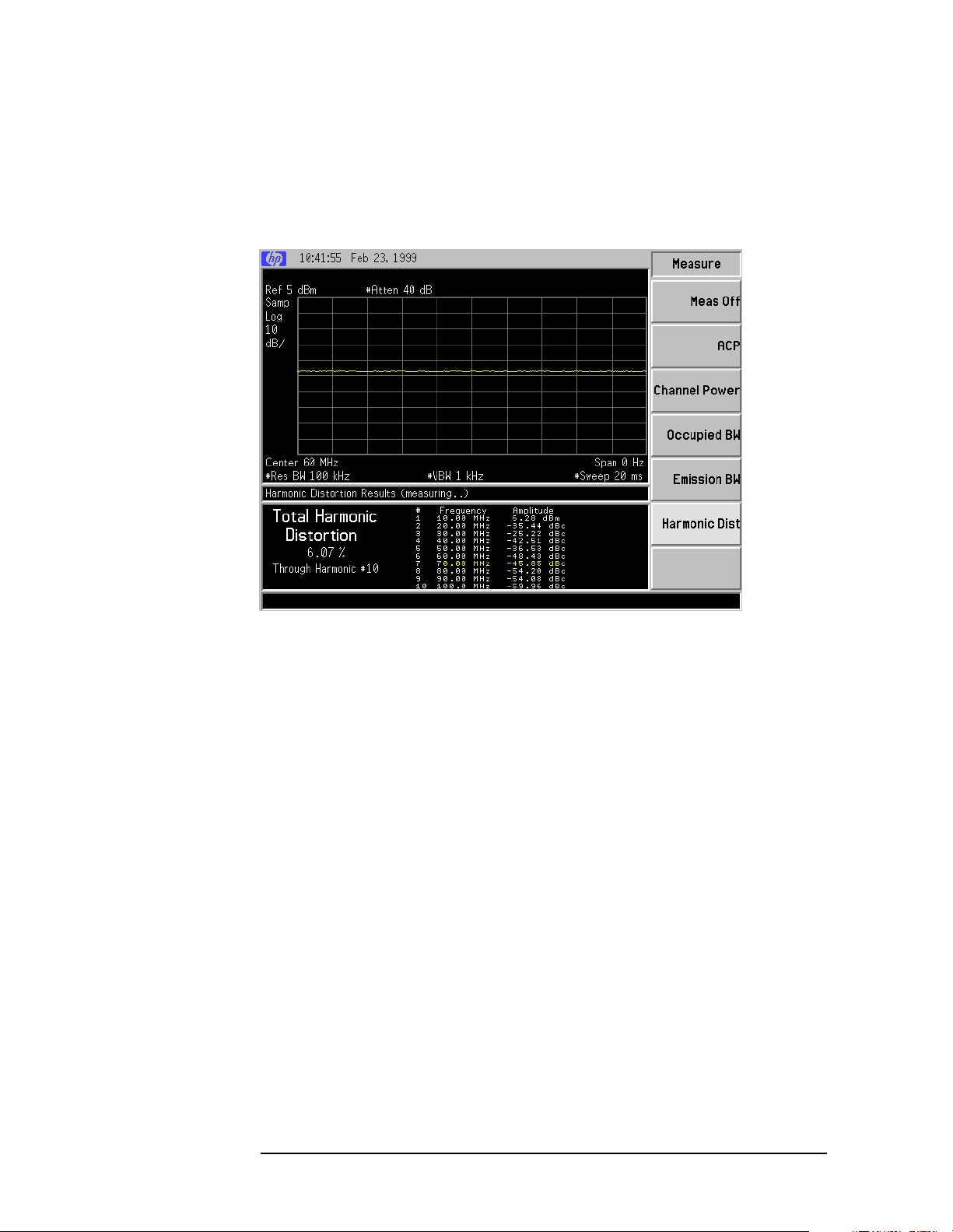
Making Measurements

Measuring Harmonics and Harmonic Distortion

8. Activate the harmonic distortion measurement by pressing

MEASURE, Harmonic Dist. The Harmonic Distortion measurement

screen will be displayed. See Figure 2-13.

Figure 2-13 Measuring the Harmonic Distortion

9. The amplitudes of the harmonics will be listed relative to the fundamental frequency. The total harmonic distortion (%THD) is also displayed.

Measurement Setup

The harmonic distortion measurement tool allows you to customize certain measurement settings. Press

Meas Setup to view the

Measurement Setup screen. See Figure 2-14.

2-22 Chapter2

Figure 2-14 Measurement Setup

Making Measurements

Measuring Harmonics and Harmonic Distortion

Avg Number allows averaging to be enabled for the harmonics.

Select the number of averages to be taken by pressing

Avg Number, 3, Enter. If 3 is selected for the average

number, the function will average the last three harmonic distortion readings. The default setting is off (no averaging). See “ST/Harmonic” below for additional information on averaging.

Harmonics allows the number of harmonics to be deﬁned. Press

Harmonics, 5, Enter, Restart, to display the fundamental

along with the second through ﬁfth harmonics. The number of harmonics selected is used to calculate the total harmonic distortion value and each harmonic value is displayed. The default value is 10.

ST/Harmonic allows the sweep time per harmonic to be modiﬁed.

Since the analyzer is placed in zero span during the measurement, the sweep time only affects the sampling period. The longer the sweep time, the more averaging is provided. ST/Harmonic provides the same functionality as Avg Number, but uses a more efﬁcient method. Press

ST/Harmonic, 400 ms, Enter to increase

the averaging. The range for this value is from 10 ms to the upper sweep time limit of the instrument.

Counter Zoom allows the analyzer to automatically zoom in on the

span while searchingfor the fundamental signal so that it can more accurately determine its frequency value. The default position is ON.

Chapter 2 2-23

Making Measurements

Measuring Harmonics and Harmonic Distortion

Measurement Control

The harmonic distortion measurement tool provides several control features. Press Meas Control to view the Measurement Control screen. See Figure 2-15.

Figure 2-15 Measurement Control

Restart allows you to restart the measurement, press

Meas Control, Restart. This has the same functionality

as the front-panel

Cont vs Single allows either continuous measurements that repeat

Restart key.

until the measurement mode is exited or a single measurement in which the analyzer stops taking data after the completion of a measurement. The default setting is continuous mode. Press

(Single) to change to single measurement mode. In

single measurement mode, press measurement. Press

Meas Control, Measure (Cont) to

Meas Control,Measure

Restart for a new

change back to continuous measurement mode.

Pause/Resume provides the ability to pause and resume the

measurement. Press measurement. Press

Meas Control, Pause to pause the Meas Control, Resume to resume

the measurement.

End of Measurement

The measurement is complete, to exit the measurement, press

Meas Off.

Measure,

2-24 Chapter2

Making Measurements

Demodulating and Viewing Television Signals (Option B7B)

Option B7B (TV Trigger and Picture on Screen) allows you to trigger the sweep of the analyzer on a speciﬁc television line of a demodulated TV waveform. Option B7B also allows you to view the television picture represented by the TV waveform on the color LCD display of the analyzer.

The following examples describe how to set the analyzer for viewing the demodulated TV waveform, viewing the TV picture, and measuring the depth of modulation of the RF carrier.

Example 1:

To set up the TV video waveform for triggering and picture viewing on the analyzer, perform the following:

1. Connect a source which contains suitable TV carrier signals (for example, terrestrial broadcast or CATV signals).

2. Press alignment process while viewing TV waveforms and TV pictures. This is necessary to prevent the background alignment process from interrupting the signal paths of the analyzer during the sweep retrace period so as to maintain a constant, uninterrupted video waveform.

NOTE After viewing the TV waveform or picture, re-enable the background

alignment process by pressing background alignment has been disabled for more than 60 minutes or the ambient temperature has changed more than 3 °C, press

Alignments, Align Now, All to ensure measurement accuracy. See the

Speciﬁcations and Characteristics Chapter for your analyzer model in the Agilent TechnologiesESA Spectrum Analyzers Speciﬁcations Guide, for information about calibration requirements.

3. Set the center frequency of the analyzer to match the TV video carrier frequency by pressing value and units.

4. Set the span to 20 MHz by pressing SPAN, 20 MHz.

System, Alignments, Auto Align, Off to disable the background

System, Alignments, Auto Align, All.Ifthe

System,

FREQUENCY, then entering the desired

5. Press

6. Adjust the reference level of the analyzer to the peak video carrier level by pressing AMPLITUDE and using the knob or step keys.

Chapter 2 2-25

Auto Couple.

Making Measurements

Demodulating and Viewing Television Signals (Option B7B)

NOTE If the signal is weak and accompanied by excessive noise, you may

choose to enable the internal preamp, if installed, to improve the signal-to-noise ratio. Press AMPLITUDE, More 1 of 2, Int Preamp (On).

7. View the spectrum. There should be a strong, “noise-like” video carrier at the center frequency, a weaker, “noise-like” chrominance sub-carrier located 3.58 MHz (NTSC standard) or 4.3 to 4.4 MHz (PAL or SECAM standards) above the video carrier, and a tightly-grouped sound carrier located 4.5 to 6.5 MHz above the video carrier. If you are viewing broadcast or cable TV signals, the lower adjacent channel sound carrier may be very close to the video carrier at the center frequency.

8. Press

BW/Avg, Resolution BW, 3 MHz to change the resolution

bandwidth of the analyzer to 3 MHz. If the test signal does not have adjacent channels present, change the resolution bandwidth to 5 MHz. However, if strong adjacent channel signals are present (primarily the sound carrier of the lower adjacent channel), set the resolution bandwidth and video bandwidth to 1 MHz.

9. Press

AMPLITUDE, Scale Type (Lin) to set the amplitude scale type of

the analyzer to Linear.

10.Press Det/Demod, Detector, Sample to set the detector mode of the analyzer to Sample.

11.Set the span to 0 Hz by pressing SPAN, Zero Span.

12.Press

AMPLITUDE and using the knob or arrow keys, adjust the

reference level so that the signal peaks are within half of a division of the top of the display.

13.Press menu: Press viewing a SECAM broadcast). Press appropriate standard for the video signal. Press

14.Press

Trig, TV Trig Setup and set the following in the TV Trig Setup

Field, Entire Frame. Press Sync (Pos) (Sync (Neg) if

Standard and then select the

TV Source, SA.

Trig, TV to enable the TV trigger. The default line number for

triggering is 17, but this can be changed to any value from 1 to 525 or from 1 to 625, depending on the selected video standard.

15.If you have Option AYX (Fast Digitized Time Domain Sweeps) or Option B7D (DSP and Fast ADC), press

Sweep, Sweep Time, 500 µs.

This allows you to view several TV lines.

A time domain display of the demodulated TV waveform will now be visible. The signals used for Figure 2-16 and Figure 2-17 were produced by a Philips PM 5518-TX Colour TV Pattern Generator.

2-26 Chapter2

Making Measurements

Demodulating and Viewing Television Signals (Option B7B)

Figure 2-16 Demodulated RF Waveform (NTSC; PAL is Similar)

Figure 2-17 Demodulated RF Waveform (SECAM)

Trig, TV is the active function, the line number used to trigger the

analyzer sweep can be changed to examine the different parts of the video waveform. The line numbering scheme varies with TV standard, but TV test patterns will often be inserted in or near line 17.

Chapter 2 2-27

Making Measurements

Demodulating and Viewing Television Signals (Option B7B)

Viewing the TV Picture

To view the TV picture, perform the following:

1. Press

Sweep, Sweep Time, 100 s to set the sweep time to 100 seconds.

The long sweep time is necessary to minimize disruption of the analog signal path during instrument retrace, which optimizes picture quality.

2. Press

Trig, TV Trig Setup, TV Monitor.

Figure 2-18 TV Picture Display

When the picture is active, you can adjust the value of the function that was active prior to enabling the picture. For example, if center frequency was the active function and the frequency step size was set to the TV channel frequency spacing, you can increment or decrement through the TV channels by pressing the step keys (⇓⇑) of the analyzer. If resolution bandwidth was the active function, you can increase or decrease the amount of ﬁltering to deal with strong adjacent channel signals.

NOTE When using the knob to vary the value of the active function, be aware

that the instrument settings will not be updated until you stop turning the knob. Make small movements of the knob with frequent pauses.

2-28 Chapter2

Making Measurements

Demodulating and Viewing Television Signals (Option B7B)

Example 2:

Measure Depth of Modulation

The depth of modulation provides a measure of the percentage of amplitude modulation (AM) on the visual carrier. With Option B7B, the analyzer can be used to measure the horizontal synchronization pulse level and vertical interval test signal (VITS) white level on an individual TV line from which a calculation of percent AM can be made. Note that this measurement method will not be valid for some types of scrambled video signals.

To perform a measurement of depth of modulation on an individual TV line, perform the following steps:

NOTE Before continuing, be sure you have performed the steps in Example 1

at the beginning of this section, “Demodulating and Viewing Television

Signals (Option B7B)” on page 2-25 to display a TV waveform on the

analyzer display with linear scaling.

1. Press

Trig, TV, and enter a line number which has a TV test signal

containing the reference white level within the waveform (100 IRE) such as the FCC, NTC-7 or ITU Composite Test Signal (typically found at or near line 17 within ﬁeld 1 or ﬁeld 2).

2. Set the sweep time to 80 µs (Option AYX or B7D required) by pressing

Sweep, Sweep Time, 80 µs. This allows viewing of a

complete TV line.

3. Set the resolution bandwidth and the video bandwidth to 1 MHz by pressing

4. Turn on video averaging by pressing entering a value of

BW/Avg, Resolution BW, 1 MHz and Video BW, 1 MHz.

BW/Avg, Average (On), and

10. This minimizes the waveform variations

caused by the presence of additional RF signals near the picture carrier, as well as waveform noise or jitter.

5. Enable the marker by pressing

Marker, Normal. Using the knob,

locate the marker within the sync tip (NTSC or PAL waveforms) or the white level (SECAM waveforms) at the top of the waveform. Alternatively, you may press

Peak Search to locate the marker on the

peak excursion.

6. Enable delta marker mode by pressing Marker, Delta. Using the knob, locate the delta marker within the white level (NTSC or PAL waveforms) or the sync tip (SECAM waveforms) at the bottom of the waveform. Alternatively, you may press

Peak Search, Min Search to

locate the delta marker on the minimum excursion of the waveform. The delta marker readout will be in percent and may have a value near 12.5%.

Chapter 2 2-29

Making Measurements

Demodulating and Viewing Television Signals (Option B7B)

Figure 2-19 Measuring Marker Delta (%) for Depth of Modulation (NTSC)

The depth of modulation (in percent) can now be determined by subtracting the marker readout (in percent) from 100. A typical value would be 87.5%.

TV Trig Setup Menu Functions

• TV Source When TV Source is set to SA, the analyzer serves to demodulate the

TV signal, thus using the analyzer as a ﬁxed tuned receiver. This allows stable, zero span sweeps of the baseband video waveform (although somewhat bandlimited by the RBW and VBW ﬁlters).

When signal may be used to produce the TV line trigger. In this case, one may use an external TV tuner to obtain the baseband waveform of the given RF carrier for triggering the analyzer sweep, allowing the analyzer to be used in a swept mode for measurements of the RF spectrum, allowing the sweep to be synchronized to the video modulation panel of the analyzer

• TV Standard Selection of a TV standard establishes the number of TV lines and

the kind of color encoding method that is used. The number of TV lines establishes the defaults for the TV line counting circuits of the analyzer and the color encoding method is used to properly set up

TV Source is set to EXT VIDEO IN, an external baseband video

. The EXT VIDEO IN connector is located on the rear

2-30 Chapter2

Table 2-1

Making Measurements

Demodulating and Viewing Television Signals (Option B7B)

the TV picture display circuits. Option B7B supports both 525 line and 625 line systems and can provide a color TV picture for NTSC and PAL color encoding methods. A black and white picture is provided for the SECAM method.

The ability to display a color picture is limited by the bandwidth settings of the analyzer (resolution bandwidth and video bandwidth). However, baseband video signals input to the EXT VIDEO IN connector on the rear panel of the analyzer are minimally ﬁltered, allowing a full color display of NTSC or PAL TV signals.

TV Standard Numberof

Lines per Frame

NTSC-M 525 60 Hz NTSC 3.58 MHz NTSC-Japan

(no pedestal) PAL-M 525 60 Hz PAL 4.43 MHz PAL-B,D,G,H,I 625 50 Hz PAL 4.43 MHz PAL-N 625 50 Hz PAL 4.43 MHz PAL-N

Combination SECAM 625 50 Hz SECAM 4.406 MHz,

•

Field

525 60 Hz NTSC 3.58 MHz

625 50 Hz PAL 3.58 MHz

Approximate Field Rate

Color Encoding Method

Color Subcarrier Frequency

4.250 MHz

A television image or frame is composed of 525 (or 625 lines) delivered in two successive ﬁelds of 262.5 (or 312.5 lines) interlaced together on a CRT when displayed.

When

Field is set to Entire Frame, the line count starts at line one in

ﬁeld one (often referred to as the “odd ﬁeld”) and ends at 525 (or 625) in ﬁeld two (often referred to as the “even ﬁeld”).

When

Field is set to Field One or Field Two, the line count begins at “1”

with the ﬁrst full line in the selected ﬁeld and ends at count 263 (or

313) for Field One, and 262 (or 312) for Field Two.

•

Sync

Analog broadcast or cable television signals are usually amplitude modulated on an RF carrier. For NTSC and PAL broadcasts, typically the RF carrier amplitude is maximized at the sync tips of the baseband video waveform and minimized at the “white” level. This results in a demodulated waveform on the analyzer where the sync pulses are on top, or positive (

Chapter 2 2-31

Sync (Pos)).

Making Measurements

Demodulating and Viewing Television Signals (Option B7B)

With SECAM broadcasts, typically the RF carrier amplitude is minimized at the sync tips of the video waveform and maximized at the “white” level. This results in a waveform on the analyzer where the sync pulses are at the bottom, or negative (

Sync (Neg)).

A normal baseband video waveform for all TV standards will have the sync tips on the bottom. When TV Source is set to Ext Video In,

Sync should be set to Neg. TV Monitor

• When TV Monitor is pressed, the picture represented by the video

waveform selected with

TV Source is presented on the LCD display of

the analyzer. The picture can only be viewed, not printed or saved. Pressing a key that normally brings up a menu restores the original graphical display with the selected menu enabled.

Fast Time Domain Sweeps

Trigger delay can be used to move the sweep trigger point arbitrarily across a given TV line or lines to allow closer examination of waveform patterns (Press

Trig, Trig Delay, and enter a delay time).

In fast sweeps (20 µs to less than 5 ms), there may be up to one trace point of variation in the start time of the waveform digitization process with respect to the actual TV trigger pulse. This randomness leads to the appearance of visual jitter on the LCD display of the analyzer. In this situation, video averaging may be used (N = 5, for example) to improve the “visual stability” of the displayed waveform. This type of jitter does not occur when sweep times are set greater than or equal to 5 ms where digitization begins less than 100 ns after the trigger pulse in that mode (much less than 1 trace point of jitter).

2-32 Chapter2

Making Measurements

Using External Millimeter Mixers (Option AYZ)

External millimeter mixers can be used to extend the frequency coverage of the E4407B spectrum analyzer. Agilent Technologies manufactures external mixers that do not require biasing and cover frequency ranges from 18 GHz to 110 GHz. Other manufacturers sell mixers that extend the range to 325 GHz, but may require biasing. The Agilent Technologies E4407B spectrum analyzer will support both types of mixers.

The Agilent Technologies E4407B spectrum analyzer contains an extensive menu of functions that help with millimeter measurements. The following examples explain how to connect external mixers to the spectrum analyzer, how to choose the band of interest, how to store and activate conversion-loss factors,and how to use the signal-identiﬁcation functions.

Figure 2-20

Example 1: Making measurements with unpreselected millimeter-wave mixers

1. Connect the signal source and harmonic mixer to the analyzer as shown in Figure 2-20.

Chapter 2 2-33

Making Measurements

Using External Millimeter Mixers (Option AYZ)

CAUTION The analyzer local oscillator output power is approximately +16 dBm.

Be sure that your external harmonic mixer can accommodate the power level before connecting it to the analyzer.

NOTE HP/Agilent 5061-5458 SMA type cables should be used to connect the

mixer IF and LO ports to the analyzer. Do not over-tighten the cables. The maximum torque should not exceed 112 N-cm (10 in-lb.)

2. On the analyzer, press external mixing by pressing

(Ext). The analyzer frequency band will be set to 26.5 – 40 GHz (A).To

choose a different band, press

Preset, Factory Preset, if present. Select

Input/Output, Input Mixer, Input Mixer

Ext Mix Band and then press the

desired band frequency range/letter key. For this example, we will use band A, which ranges from 26.5 GHz to 40 GHz.

3. To correct for the conversion-loss of the harmonic mixer in use, the analyzer amplitude correction feature is used. Access this feature by pressing,

AMPLITUDE Y Scale, More1of2, Corrections, Modify, Select.

Select a correction set for use with external mixing. The recommended set to use is used. Press

Edit to enter the appropriate conversion loss data for the

Other although any available set could be

mixer in use. On the HP/Agilent 11970 harmonic mixers, these values are listed on the mixer. A single average value could be entered for the entire band by using only a single correction value. More correction points entered across the band in use will improve frequency response accuracy. Up to 200 points may be deﬁned for each set. Once the desired correction points are entered, press

Return, Correction (On) to activate correction set Other. This will also

turn corrections on resulting in a calibrated display. It is recommended that the correction set entered be saved on the internal memory or the ﬂoppy drive for future reference.

4. The IF output of a harmonic mixer will contain a signal at the intermediate frequency of the analyzer whenever the harmonic frequency of the LO and the frequency of the RF differ by the intermediate frequency. As a result, within a single harmonic band, a single input signal can produce multiple responses on the analyzer display, only one of which is valid (see Figure 2-21). These responses come in pairs, where members of the valid response pair are separated by 642.8 MHz and either the right-most (for negative harmonics) or left-most (for positive harmonics) member of the pair is the correct response.

2-34 Chapter2

Figure 2-21

Making Measurements

Using External Millimeter Mixers (Option AYZ)

5. Identiﬁcation of valid responses is achieved by simply turning on the signal-identiﬁcation feature. ( identiﬁcation mode.) Press

Signal Ident (On) and note that now only the valid response (35 GHz)

remains. Refer to Figure 2-22. Press

Preset selects the Image Supress signal

Input/Output, Input Mixer,

Peak Search to place a marker

on the remaining response. The signal-identiﬁcation routine can introduce slight amplitude errors which is indicated by the message Signal Ident On, Amptd Uncal. After identifying a signal of interest, press

Signal Ident (Off) before making ﬁnal amplitude

measurements.

Chapter 2 2-35

Figure 2-22

Making Measurements

Using External Millimeter Mixers (Option AYZ)

6. The HP/Agilent 11970 Series harmonic mixers do not require bias. Mixers requiring bias can also be used with the E4407B. Generally, the conversion loss calibration data for mixers requiring bias, will be most accurate when the correct bias conditions are present. Set the bias as follows:

a. To measure a signal, access external mixing and set the band as

described previously.

b. To activate bias press

Mixer Bias (On). A +I or –I will appear in the display annotation

Input/Output, Input Mixer, Mixer Conﬁg,

indicating bias is on.

c. Enter the desired bias current in mA with the data control keys.

WARNING The open-circuit bias voltage can be as great as ±3.5V through a

source resistance of 500 ohms. Such voltage levels may appear when recalling an instrument state in which a bias setting has been stored.

NOTE The bias value that appears on the analyzer display is expressed in

terms of short-circuit current (that is, the current that would ﬂow if the

IF INPUT were shorted to ground). The actual current ﬂowing into the

mixer will be less.

2-36 Chapter2

Figure 2-23

Making Measurements

Using External Millimeter Mixers (Option AYZ)

Example 2: Making Measurements with HP/Agilent 11974 Series Preselected Millimeter-Wave Mixers

1. Connect the signal source and preselected mixer to the analyzer as shown in Figure 2-23.

Frequency Tracking Calibration

This procedure is used to align the frequency of the preselector ﬁlter of the HP/Agilent 11974 to the tuned frequency of the analyzer. This procedure should be followed any time that the HP/Agilent 11974 is connected to a different analyzer. The calibration should be periodically checked.

1. Set the HP/Agilent 11974 rear-panel switches “HP/Agilent 70907B” and “LEDS” to the ON position, and the other two switches to the OFF position, in order for the HP/Agilent 11974 to properly scale to the tune signal of the analyzer.

2. Conﬁgure the analyzer for a preselected external mixer by pressing the following keys:

Preset, Factory Preset (if present), Input/Output, Input Mixer (Ext), Mixer Conﬁg, Mixer Type (Presel)

3. Set the desired band of operation. Press Ext Mix Band, A, Q, U, or V. (Note that only A,Q,U, and V bands are available.)

Chapter 2 2-37

Making Measurements

Using External Millimeter Mixers (Option AYZ)

4. Set the Presel Adjust to 0 MHz by pressing AMPLITUDE, Presel

Adjust, 0 MHz.

5. Set the analyzer to zero span by pressing

6. Set the analyzer center frequency by pressing

Freq, and enter the corresponding value for the appropriate mixer.

SPAN, Zero Span.

FREQUENCY, Center

(Refer to Table 2-2) On the rear panel of the HP/Agilent 11974, adjust the corresponding potentiometer until one or both of the green LEDs are lit.

Table 2-2

Mixer HP/Agilent P/N

11974A 26.5 GHz “26.5 GHz Adjust” 11974Q 33.0 GHz “33.0 GHz Adjust” 11974U 40.0 GHz “40.0 GHz Adjust” 11974V 50.0 GHz “50.0 GHz Adjust”

Analyzer Center Frequency

Potentiometer

7. Change the analyzer center frequency to the value indicated in

Table 2-3 and again adjust the corresponding potentiometer on the

rear panel of the HP 11974 until one or both of the green LEDs are lit.

Table 2-3

Mixer HP/Agilent P/N

11974A 40.0 GHz “40.0 GHz Adjust” 11974Q 50.0 GHz “50.0 GHz Adjust” 11974U 60.0 GHz “60.0 GHz Adjust” 11974V 75.0 GHz “75.0 GHz Adjust”

Analyzer Center Frequency

Potentiometer

8. Repeat steps 6 and 7 until the green LEDs are lit at both frequencies without additional adjustments.

2-38 Chapter2

Making Measurements

Using External Millimeter Mixers (Option AYZ)

Band Selection

1. If necessary, conﬁgure the analyzer for preselected external mixing by pressing the following keys:

Input/Output, Input Mixer (Ext), Mixer Conﬁg, Mixer Type (Presel)

2. If necessary, adjust the tracking of the HP/Agilent 11974 to the analyzer being used for preselected external mixing, by using the Frequency Tracking Calibration procedure above.

3. Press the following keys to select the desired mixing band: (In this example, we will use an HP/Agilent 11974Q (33.0 to 50.0 GHz) to view a 40 GHz, -15 dBm signal.)

Input/Output, Input Mixer, Ext Mix Band, 33-50 GHz (Q)

Amplitude Calibration

1. Enter the conversion-loss versus frequency data from either the calibration label on the bottom of the HP/Agilent 11974, or the supplied calibration sheet by using the procedure in step 3 of Example 1. The full Q-band is displayed in Figure 2-24.

Figure 2-24

Chapter 2 2-39

Making Measurements

Using External Millimeter Mixers (Option AYZ)

2. To complete the amplitude calibration process, the preselector must be adjusted at each frequency of interest. Before making ﬁnal amplitude measurements with the analyzer, perform the following:

a. Place a marker on the signal of interest.

Figure 2-25

b. Press c. Press

SPAN, Span Zoom, 10 MHz to zoom in on the signal. AMPLITUDE, Presel Center.

The ﬁnal amplitude measurement can now be read out with the marker. See Figure 2-25.

2-40 Chapter2

Agilent E4401B Measurement Guide

Specifications and Main Features

Frequently Asked Questions

User Manual

Contents

1 Making Basic Measurements

What is in This Chapter

Comparing Signals

Example 1:

Example 2:

Resolving Signals of Equal Amplitude

Example:

Resolving Small Signals Hidden by Large Signals

Example:

Making Better Frequency Measurements

Example:

Decreasing the Frequency Span Around the Signal

Example:

Tracking Drifting Signals

Example 1:

Example 2:

Measuring Low Level Signals

Example 1:

Example 2:

Example 3:

Example 4:

Identifying Distortion Products

Distortion from the Analyzer

Third-Order Intermodulation Distortion

Measuring Signal-to-Noise

Making Noise Measurements

Example 1:

Example 2:

Example 3:

Example 4:

Demodulating AM Signals (Using the Analyzer As a Fixed Tuned Receiver)

Example:

Demodulating FM Signals (Without Option BAA)

Example:

2 Making Measurements

What’s in This Chapter

Making Stimulus Response Measurements

What Are Stimulus Response Measurements?

Using An Analyzer With A Tracking Generator

Stepping Through a Transmission Measurement

Tracking Generator Unleveled Condition

Measuring Device Bandwidth

Example:

Measuring the Return Loss

Demodulating and Listening to an AM Signal

Example 1:

Example 2:

Measuring Harmonics and Harmonic Distortion

Example:

Demodulating and Viewing Television Signals (Option B7B)

Example 1:

Example 2:

TV Trig Setup Menu Functions

Using External Millimeter Mixers (Option AYZ)

Example 1: Making measurements with unpreselected millimeter-wave mixers

Example 2: Making Measurements with HP/Agilent 11974 Series Preselected Millimeter-Wave Mixers