Agilent 8703B User Manual

Agilent 8703B Lightwave
Component Analyzer

User’s Guide

© Copyright
Agilent Technologies 2001
All Rights Reserved. Repro­duction, adaptation, or transla­tion without prior w r itt en
permission is prohibit ed ,
except as allowed under copy­right laws.

Agilent Part No. 08703- 90 20 1
Printed in USA
July 2001

Agilent Technologies
Lightwave Division
3910 Brickway BoulevardSanta
Rosa, CA 95403, USA

Notice.

The information contained in
this document is subject to
change without notice. Compa­nies, names, and data used in
examples herein are fictitious
unless otherwise noted. Agi­lent Technologies makes no
warranty of any kind with
regard to this material, includ­ing but not limited to, the
implied warranties of mer­chantability and fitness for a
particular purpose. Agilent
Technologies shall not be liable
for errors contained herein or
for incidental or consequential
damages in connection with
the furnishing, performance, or
use of this material.

Restricted Rights Legend.

Use, duplication, or disclosure
by the U.S. Government is sub­ject to restrictions as set forth
in subparagrap h (c) (1 ) (i i) of
the Rights in Technical Data
and Computer Software clause
at DFARS 252.227-7013 for
DOD agencies, and subpara­graphs (c) (1) and (c) (2) of
the Commercial Computer
Software Restricted Rights
clause at FAR 52.227-19 for
other agencies.

Warranty.

This Agilent Technologies
instrument product is war­ranted against defects in mate­rial and workmanship for a
period of one yea r fro m date of
shipment. During the war­ranty period, Agilent Technolo­gies will, at its option, either
repair or replace products
which prove to be defective.
For warranty service or repair,
this product must be returned
to a service facility designated
by Agilent Technologies. Buyer
shall prepay shipping charges
to Agilent Technologies and
Agilent Technologies shall pay
shipping charges to return the
product to Buyer. However,
Buyer shall pay all shipping
charges, duties, and taxes for
products returned to Agilent
Technologies from another
country.

Agilent Technologies warrants
that its software and firmware
designated by Agilent Technol­ogies for use with an instru­ment will execute its
programming instructions
when properly installed on that
instrument. Agilent Technolo­gies does not warrant that the
operation of the instrument, or
software, or firmware will be
uninterrupted or error-free.

Limitation of Warranty.

The foregoing warranty shall
not apply to defects resulting
from improper or inadequate
maintenance by Buyer,
Buyer-supplied software or
interfacing, unauthorized mod­ification or misuse, operation
outside of the environmental
specifications for the product,
or improper site preparation or
maintenance.

No other warranty is
expressed or implied. Agilent
Technologies specifically dis­claims the implied warranties
of merchantability and fitness
for a particular purpose.

Exclusive Remedies.

The remedies provided herein
are buyer's sole and exclusive
remedies. Agilent Technologies
shall not be liable for any
direct, indirect, special, inci­dental, or consequential dam­ages, whether based on
contract, tort, or any other
legal theory.

Safety Symbols.

CAUTION
The caution sign denotes a

hazard. It calls attention to a
procedure which, if not cor­rectly performed or adhered
to, could result in damage to or
destruction of the product. Do
not proceed beyond a caution
sign until the indicated condi­tions are fully understood and
met.

WARNING
The warning sign denotes a

hazard. It calls attention to a
procedure which, if not cor­rectly performed or adhered
to, could result in injury or loss
of life. Do not proceed beyond
a warning sign until the indi­cated conditions are fully
understood and met.

The instruction man­ual symbol. The prod­uct is marked with this
warning symbol when
it is necessary for the
user to refer to the
instructions in the
manual.

The laser radiation
symbol. This warning
symbol is marked on
products which have a
laser output.

The AC symbol is used
to indicate the required
nature of the line mod­ule input power.

| The ON symbols are

used to mark the posi­tions of the instrument
power line switch.

❍ The OFF symbols

are used to mark the
positions of the instru­ment power line
switch.

The CE mark is a regis­tered trademark of the
European Community.

The CSA mark is a reg­istered trademar k of
the Canadian Stan­dards Association.

The C-Tick mark is a
registered trademark of
the Australian Spec­trum Management
Agency.

This text denotes the

ISM1-A

instrument is an Indus­trial Scientific and
Medical Group 1 Class
A product.

Typographical C on ve nt io ns.

The following conventions are
used in this book:

Key type for keys or text lo cated
on the keyboard or ins tr ume nt.

Softkey type for key names that
are displayed on the instru­ment’s screen.

Display type for words or

characters displayed on the
computer’s screen or instru­ment’s display.

User type for words or charac-

ters that you type or enter.
Emphasis type for words or

characters that emphasize
some point or that are used as
place holders for text that you
type.

2

Contents

1. Connector Care & ESD Information

Cleaning Connections for Accurate Measurements 1-2
Caring for Electrical Connections 1-11
Electrostatic Discharge Information 1-12

2. Making Measurements

Making Measurements 2-2
Making a Basic Measurement 2-3
Using Display Functions 2-4
Using Markers 2-17
Using the List Mode to Test a Device 2-37
Using Limit Lines to Test a Device 2-42
Using Ripple Limits to Test a Device 2-50
Using Bandwidth Limits to Test a Bandpass Filter 2-60
Using Test Sequencing 2-66
Using Test Sequencing to Test a Device 2-77
Magnitude and Phase Comparisons of Lightwave Receivers 2-83
Mathematically Combining Device Responses 2-91
Using a Coefficient Model for Device Response and Design Model Comparison 2-95
Using an External Laser 2-98

3. Optimizing Measurement Results

Optimizing Measurement Results 3-2
Taking Care of Connectors 3-3
Increasing Measurement Accuracy 3-4
Increasing Dynamic Range 3-7
Reducing Noise 3-8
Reducing Receiver Crosstalk 3-9

4. Calibrating for Increased Measurement Accuracy

Calibrating for Increased Measurement Accuracy 4-2
Calibration Considerations 4-3
Procedures for Error Correcting Your Measurements 4-9
O/O Response Calibration 4-11
O/O Response and Isolation Calibration 4-13
E/O Response Calibration 4-16
E/O Reflection Sensitivity Calibration 4-17
E/O Response and Isolation Calibration 4-18
E/O Response and Match Calibration 4-20
O/E Response Calibration 4-23
O/E Response and Isolation Calibration 4-24
O/E Response and Match Calibration 4-26
Modifying Lightwave Calibration Kits 4-29
Modifying an Electrical Calibration Kit 4-30
Ver i fy Per formance 4 - 39

Contents-1

Contents

5. Verifying Measurement Accuracy

Verifying Measurement Accuracy 5-2
Agilent Technologies Service Offices 5-8

6. Saving and Recalling Measurements and Data

Saving and Recalling Measurements and Data 6-2
Saving and Recalling Instrument States 6-3
Saving an Instrument State 6-5
Saving Measurement Results 6-6
Re-Saving an Instrument State 6-18
Deleting a File 6-19
Renaming a File 6-20
Recalling a File 6-21
Formatting a Disk 6-22
Solving Problems with Saving or Recalling Files 6-23

7. Printing Measurement Results

Printing Measurements Results 7-2
Printing or Plotting Your Measurement Results 7-3
Configuring a Print Function 7-4
Defining a Print Function 7-6
Printing One Measurement Per Page 7-8
Printing Multiple Measurements Per Page 7-9
Configuring a Plot Function 7-10
Defining a Plot Function 7-15
Plotting One Measurement Per Page Using a Pen Plotter 7-19
Plotting Multiple Measurements Per Page Using a Pen Plotter 7-20
To View Plot Files on a PC 7-22
Outputting Plot Files from a PC to a Plotter 7-23
Outputting Plot Files from a PC to an HPGL Compatible Printer 7-24
Outputting Single Page Plots Using a Printer 7-26
Outputting Multiple Plots to a Single Page Using a Printer 7-27
Plotting Multiple Measurements Per Page from Disk 7-28
Titling the Displayed Measurement 7-32
Configuring the Analyzer to Produce a Time Stamp 7-33
Aborting a Print or Plot Process 7-34
Printing or Plotting the List Values or Operating Parameters 7-35
Solving Problems with Printing or Plotting 7-36

Contents-2

1

Cleaning Connections for Accurate Measurements 1-2

Choosing the Right Connector 1-2
Inspecting Connectors 1-4
Cleaning Connectors 1-8

Caring for Electrical Connections 1-11
Electrostatic Discharge Information 1-12
Reducing ESD Damage 1-13

Connector Care & ESD Information

Connector Care & ESD Information
Cleaning Connections for Accurate Measurements

Cleaning Connections for Accurate Measurements

Today, advances in measurement capabilities make connectors and connection techniques more
important than ever. Damage to the connectors on calibration and verification devices, test ports,
cables, and other devices can degrade measurement accuracy and damage instruments. Replacing a
damaged connector can cost thousands of dollars, not to mention lost time! This expense can be
avoided by observing the simple precautions presented in this document. This document also contains
a brief list of tips for caring for electrical connectors.

Choosing the Right Connector

A critical but often overlooked factor in making a good lightwave measurement is the selection of the
fiber-optic connector. The differences in connector types are mainly in the mechanical assembly that
holds the ferrule in position against another identical ferrule. Connectors also vary in the the polish,
curve, and concentricity of the core within the cladding. Mating one style of cable to another requires
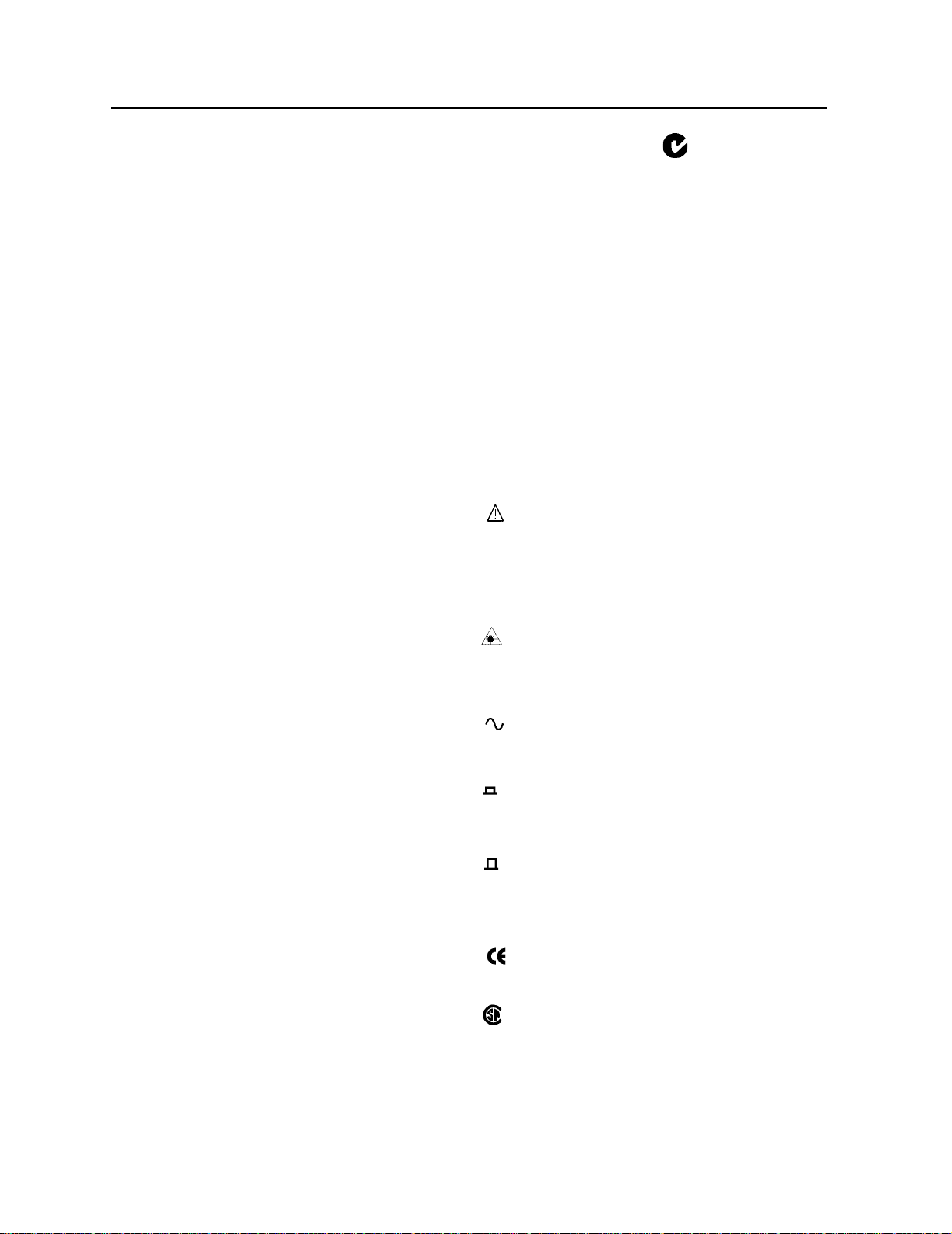
an adapter. Agilent Technologies offers adapters for most instruments to allow testing with many dif­ferent cables. The Figure 1-1 on page 1-3 shows the basic components of a typical connectors.

The system tolerance for reflection and insertion loss must be known when selecting a connector from
the wide variety of currently available connectors. Some items to consider when selecting a connector
are:

• How much insertion loss can be allowed?

• Will the connector need to make multiple connections? Some connectors are better than
others, and some are very poor for making repeated connections.

• What is the reflection tolerance? Can the system take reflection degradation?

• Is an instrument-grade connector with a precision core alignment required?

• Is repeatability tolerance for reflection and loss important? Do your specifications take
repeatability uncertainty into account?

• Will a connector degrade the return loss too much, or will a fusion splice be required? For
example, many DFB lasers cannot operate with reflections from connectors. Often as
much as 90 dB isolation is needed.

1-2

Connector Care & ESD Information

Cleaning Connections for Accurate Measurements

Figure 1-1. Basic components of a connector.

Over the last few years, the FC/PC style connector has emerged as the most popular connector for
fiber-optic applications. While not the highest performing connector, it represents a good compromise
between performance, reliability, and cost. If properly maintained and cleaned, this connector can
withstand many repeated connections.

However, many instrument specifications require tighter tolerances than most connectors, including
the FC/PC style, can deliver. These instruments cannot tolerate connectors with the large non-concen­tricities of the fiber common with ceramic style ferrules. When tighter alignment is required,
Agilent instruments typically use a connector such as the Diamond HMS-10, which has concentric tol­erances within a few tenths of a micron. Agilent then uses a special universal adapter, which allows
other cable types to mate with this precision connector. See Figure 1-2.

Figure 1-2. Universal adapters to Diamond HMS-10

The HMS-10 encases the fiber within a soft nickel silver (Cu/Ni/Zn) center which is surrounded by a
tough tungsten carbide casing, as shown in Figure 1-3 on page 1-4.

1-3

Connector Care & ESD Information
Cleaning Connections for Accurate Measurements

Figure 1-3. Cross-section of the Diamond HMS-10 connector.

The nickel silver allows an active centering process that permits the glass fiber to be moved to the
desired position. This process first stakes the soft nickel silver to fix the fiber in a near-center loca-

tion, then uses a post-active staking to shift the fiber into the desired position within 0.2 µm. This pro-

cess, plus the keyed axis, allows very precise core-to-core alignments. This connector is found on most
Agilent lightwave instruments.

The soft core, while allowing precise centering, is also the chief liability of the connector. The soft
material is easily damaged. Care must be taken to minimize excessive scratching and wear. While
minor wear is not a problem if the glass face is not affected, scratches or grit can cause the glass fiber
to move out of alignment. Also, if unkeyed connectors are used, the nickel silver can be pushed onto
the glass surface. Scratches, fiber movement, or glass contamination will cause loss of signal and
increased reflections, resulting in poor return loss.

Inspecting Connectors

Because fiber-optic connectors are susceptible to damage that is not immediately obvious to the naked
eye, bad measurements can be made without the user even being aware of a connector problem.
Although microscopic examination and return loss measurements are the best way to ensure good
connections, they are not always practical. An awareness of potential problems, along with good
cleaning practices, can ensure that optimum connector performance is maintained. With
glass-to-glass interfaces, it is clear that any degradation of a ferrule or the end of the fiber, any stray
particles, or finger oil can have a significant effect on connector performance.

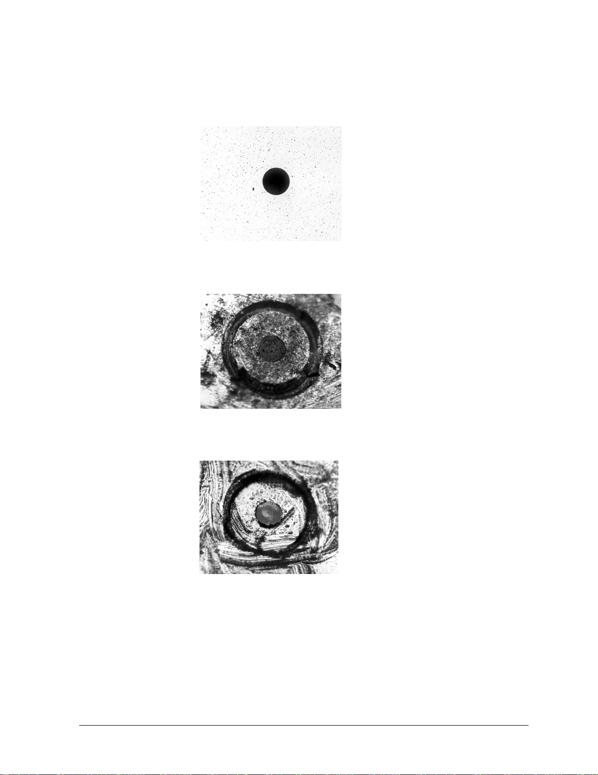
Figure 1-4 shows the end of a clean fiber-optic cable. The dark circle in the center of the micrograph is

the fiber’s 125 µm core and cladding which carries the light. The surrounding area is the soft

nickel-silver ferrule. Figure 1-5 shows a dirty fiber end from neglect or perhaps improper cleaning.
Material is smeared and ground into the end of the fiber causing light scattering and poor reflection.
Not only is the precision polish lost, but this action can grind off the glass face and destroy the connec­tor.

1-4

Connector Care & ESD Information

Cleaning Connections for Accurate Measurements

Figure 1-6 shows physical damage to the glass fiber end caused by either repeated connections made

without removing loose particles or using improper cleaning tools. When severe, the damage on one
connector end can be transferred to another good connector that comes in contact with it.

Figure 1-4. Clean, problem-free fiber end and ferrule.

Figure 1-5. Dirty fiber end and ferrule from poor cleaning.

Figure 1-6. Damage from improper cleaning.

The cure for these problems is disciplined connector care as described in the following list and in

“Cleaning Connectors” on page 1-8.

Use the following guidelines to achieve the best possible performance when making measurements on
a fiber-optic system:

•Never use metal or sharp objects to clean a connector and never scrap e th e conn ect or.

•Avoid matching gel and oils.

1-5

Connector Care & ESD Information
Cleaning Connections for Accurate Measurements

While these often work well on first insertion, they are great dirt magnets. The oil or gel grabs and
holds grit that is then ground into the end of the fiber. Also, some early gels were designed for use
with the FC, non-contacting connectors, using small glass spheres. When used with contacting connec­tors, these glass balls can scratch and pit the fiber. If an index matching gel or oil must be used, apply
it to a freshly cleaned connector, make the measurement, and then immediately clean it off. Never use
a gel for longer-term connections and never use it to improve a damaged connector. The gel can mask
the extent of damage and continued use of a damaged fiber can transfer damage to the instrument.

• When inserting a fiber-optic cable into a connector, gently insert it in as straight a line as
possible. Tipping and inserting at an angle can scrape material off the inside of the
connector or even break the inside sleeve of connectors made with ceramic material.

• When inserting a fiber-optic connector into a connector, make sure that the fiber end does
not touch the outside of the mating connector or adapter.

• Avoid over tightening connections.

Unlike common electrical connections, tighter is not better. The purpose of the connector is to bring
two fiber ends together. Once they touch, tightening only causes a greater force to be applied to the
delicate fibers. With connectors that have a convex fiber end, the end can be pushed off-axis resulting
in misalignment and excessive return loss. Many measurements are actually improved by backing off
the connector pressure. Also, if a piece of grit does happen to get by the cleaning procedure, the
tighter connection is more likely to damage the glass. Tighten the connectors just until the two fibers
touch.

• Keep connectors covered when not in use.

• Use fusion splices on the more permanent critical nodes. Choose the best connector
possible. Replace connecting cables regularly. Frequently measure the return loss of the
connector to check for degradation, and clean every connector, every time.

All connectors should be treated like the high-quality lens of a good camera. The weak link in instru­ment and system reliability is often the inappropriate use and care of the connector. Because current
connectors are so easy to use, there tends to be reduced vigilance in connector care and cleaning. It
takes only one missed cleaning for a piece of grit to permanently damage the glass and ruin the con­nector.

Measuring insertion loss and return l oss

Consistent measurements with your lightwave equipment are a good indication that you have good
connections. Since return loss and insertion loss are key factors in determining optical connector per­formance they can be used to determine connector degradation. A smooth, polished fiber end should
produce a good return-loss measurement. The quality of the polish establishes the difference between
the “PC” (physical contact) and the “Super PC” connectors. Most connectors today are physical con­tact which make glass-to-glass connections, therefore it is critical that the area around the glass core
be clean and free of scratches. Although the major area of a connector, excluding the glass, may show
scratches and wear, if the glass has maintained its polished smoothness, the connector can still pro­vide a good low level return loss connection.

If you test your cables and accessories for insertion loss and return loss upon receipt, and retain the
measured data for comparison, you will be able to tell in the future if any degradation has occurred.
Typical values are less than 0.5 dB of loss, and sometimes as little as 0.1 dB of loss with high perfor­mance connectors. Return loss is a measure of reflection: the less reflection the better (the larger the
return loss, the smaller the reflection). The best physically contacting connectors have return losses
better than 50 dB, although 30 to 40 dB is more common.

1-6

Connector Care & ESD Information

Cleaning Connections for Accurate Measurements

To Test Insertion Loss

Use an appropriate lightwave source and a compatible lightwave receiver to test insertion loss. Exam­ples of test equipment configurations include the following equipment:

• HP/Agilent 71450A or 71451A Optical Spectrum Analyzers with Option 002 built-in white
light source.

• HP/Agilent 8702 or 8703 Lightwave Component Analyzer system.

• HP/Agilent 83420 Chromatic Dispersion Test Set with an HP/Agilent 8510 analyzer.

• HP/Agilent 8153 Lightwave Multimeter with a source and power sensor module.

To Test Return Loss

Use an appropriate lightwave source, lightwave receiver, and lightwave coupler to test return loss.
Examples of test equipment configurations include the following equipment:

• HP/Agilent 8703 Lightwave Component Analyzer.

• HP/Agilent 8702 Lightwave Component Analyzer with the appropriate source, receiver,
and lightwave coupler.

• HP/Agilent 8504 Precision Reflectometer.

• HP/Agilent 8153 Lightwave Multimeter with a source and power sensor module in
conjunction with a lightwave coupler.

• HP/Agilent 81554SM Dual Source and HP/Agilent 81534A Return Loss Module.

Visual inspection of fiber ends

Visual inspection of fiber ends can be helpful. Contamination or imperfections on the cable end face
can be detected as well as cracks or chips in the fiber itself. Use a microscope (100X to 200X magnifi­cation) to inspect the entire end face for contamination, raised metal, or dents in the metal as well as
any other imperfections. Inspect the fiber for cracks and chips. Visible imperfections not touching the
fiber core may not affect performance (unless the imperfections keep the fibers from contacting).

WARNING Always remove both ends of fiber-optic cables from any instrument, system,

or device before visually inspecting the fiber ends. Disable all optical
sources before disconnecting fiber-optic cables. Failure to do so may result
in permanent injury to your eyes.

1-7

Connector Care & ESD Information
Cleaning Connections for Accurate Measurements

Cleaning Connectors

The procedures in this section provide the proper steps for cleaning fiber-optic cables and Agilent uni­versal adapters. The initial cleaning, using the alcohol as a solvent, gently removes any grit and oil. If a
caked-on layer of material is still present, (this can happen if the beryllium-copper sides of the ferrule
retainer get scraped and deposited on the end of the fiber during insertion of the cable), a second
cleaning should be performed. It is not uncommon for a cable or connector to require more than one
cleaning.

CAUTION Agilent Technologies strongly recommends that index matching compounds not

be applied to their instruments and accessories. Some compounds, such as gels,
may be difficult to remove and can contain damaging particulates. If you think
the use of such compounds is necessary, refer to the compound manufacturer
for information on application and cleaning procedures.

Table 1-1. Cleaning Accessories

Item Agilent Part Number

Pure isopropyl alcohol —
Cotton swabs 8520-0023
Small foam swabs 9300-1223
Compressed dust remover (non-residue) 8500-5262

Table 1-2. Dust Caps Provided with Lightwave Instruments

Item Agilent Part Number

Laser shutter cap 08145-64521
FC/PC dust cap 08154-44102
Biconic dust cap 08154-44105
DIN dust cap 5040-9364
HMS10/Agilent dust cap 5040-9361
ST dust cap 5040-9366

1-8

Connector Care & ESD Information

Cleaning Connections for Accurate Measurements

To clean a non-lensed connector

CAUTION Do not use any type of foam swab to clean optical fiber ends. Foam swabs can

leave filmy deposits on fiber ends that can degrade performance.

1. Apply pure isopropyl alcohol to a clean lint-free cotton swab or lens paper.

Cotton swabs can be used as long as no cotton fibers remain on the fiber end after
cleaning.

2. Clean the ferrules and other parts of the connector while avoiding the end of the fiber.

3. Apply isopropyl alcohol to a new clean lint-free cotton swab or lens paper.

4. Clean the fiber end with the swab or lens paper.

5. Do not scrub during this initial cleaning because grit can be caught in the swab and
become a gouging element.

6. Immediately dry the fiber end with a clean, dry, lint-free cotton swab or lens paper.

7. Blow across the connector end face from a distance of 6 to 8 inches using filtered, dry,
compressed air. Aim the compressed air at a shallow angle to the fiber end face.

8. Nitrogen gas or compressed dust remover can also be used.

CAUTION Do not shake, tip, or invert compressed air canisters, because this releases

particles in the can into the air. Refer to instructions provided on the
compressed air canister.

9. As soon as the connector is dry, connect or cover it for later use.

If the performance, after the initial cleaning, seems poor tr y cleaning the connector again. Often a sec­ond cleaning will restore proper performance. The second cleaning should be more arduous with a
scrubbing action.

1-9

Connector Care & ESD Information
Cleaning Connections for Accurate Measurements

To clean an adapter

The fiber-optic input and output connectors on many Agilent instruments employ a universal adapter
such as those shown in the following picture. These adapters allow you to connect the instrument to
different types of fiber-optic cables.

Figure 1-7. Universal adapters

1. Apply isopropyl alcohol to a clean foam swab.

Cotton swabs can be used as long as no cotton fibers remain after cleaning. The foam
swabs listed in this section’s introduction are small enough to fit into adapters.

Although foam swabs can leave filmy deposits, these deposits are very thin, and the risk
of other contamination buildup on the inside of adapters greatly outweighs the risk of
contamination by foam swabs.

2. Clean the adapter with the foam swab.

3. Dry the inside of the adapter with a clean, dry, foam swab.

4. Blow through the adapter using filtered, dry, compressed air.

Nitrogen gas or compressed dust remover can also be used. Do not shake, tip, or invert compressed air can­isters, because this releases particles in the can into the air. Refer to instructions provided on the com­pressed air canister.

1-10

Connector Care & ESD Information

Caring for Electrical Connections

Caring for Electrical Connections

The following list includes the basic principles of microwave connector care. For more information on
microwave connectors and connector care, consult the Hewlett-Packard Microwave Connector Care
Manual, HP part number 08510-90064.

Handling and Storage

• Keep connectors clean

• Extend sleeve or connect or nut

• Use plastic endcaps during stor ag e

• Do not touch mating plane surfaces

• Do not set connectors contact-end down

Visual Inspection

• Inspect all connectors carefully before every connection

• Look for metal particles, scratches, and dents

• Do not use damaged connectors

Cleaning

• Try cleaning with compre ssed air first

• Clean the connector threads

• Do not use abrasives

• Do not get liquid onto the plastic support beads

Making Connections

• Align connectors carefully

• Make prelimi nary conne ct ion light ly

• To tighten, turn connector nut only

• Do not ap ply bending forc e to connection

• Do not overtighten preliminary conn ec tion

• Do not tw ist or screw in conn ec tors

• Do not tig hte n past the “break” point of the tor que wrench

1-11

Connector Care & ESD Information
Electrostatic Discharge Information

Electrostatic Discharge Information

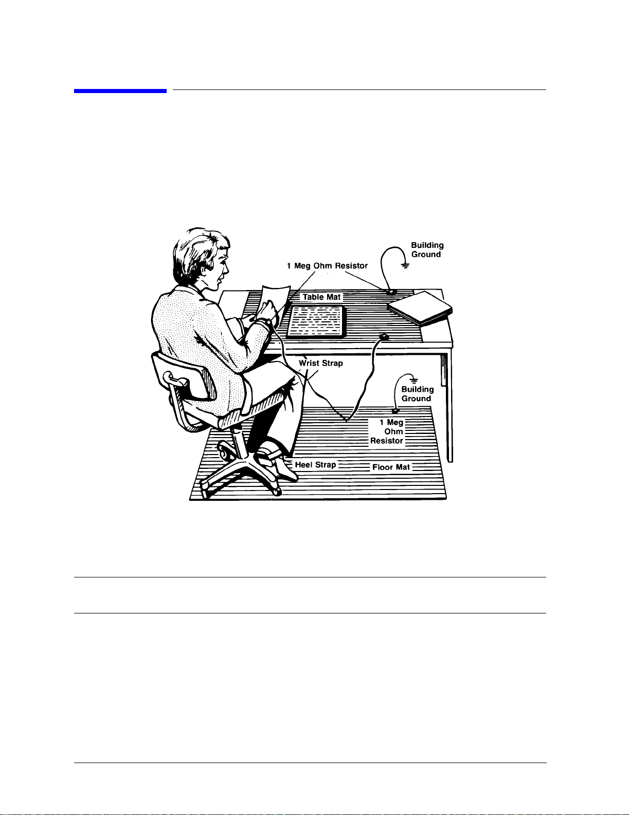
Electrostatic discharge (ESD) can damage or destroy electronic components. All work on electronic
assemblies should be performed at a static-safe work station. The following figure shows an example
of a static-safe work station using two types of ESD protection:

•Conductive table-mat and wrist-strap combination.

•Conductive floor-mat and heel-strap combination.

Both types, when used together, provide a significant level of ESD protection. Of the two, only the
table-mat and wrist-strap combination provides adequate ESD protection when used alone.

To ensure user safety, the static-safe accessories must provide at least 1 MΩ of isolation from ground.

Refer to Table 1-3 on page 1-13 for information on ordering static-safe accessories.

WARNING These techniques for a static-safe work station should not be used when

working on circuitry with a voltage potential greater than 500 volts.

1-12

Connector Care & ESD Information
Electrostatic Discharge Information

Reducing ESD Damage

The following suggestions may help reduce ESD damage that occurs during testing and servicing oper­ations.

• Personnel should be grounded with a resistor-isolated wrist strap before removing any
assembly from the unit.

• Be sure all instruments are properly earth-grounded to prevent a buildup of static charge.

Table 1-3. Static-Safe Accessories

Agilent Part
Number

9300-0797

9300-0980 Wrist-strap cord 1.5 m (5 ft)
9300-1383 Wrist-strap, color black, stainless steel, withoutcord, has four adjustable

9300-1169 ESD heel-strap (reusable 6 to 12 months).

Description

Set includes: 3M static control mat 0.6 m
ft) ground wire. (The wrist-strap andwrist-strap cord are not included. They
must be ordered separately.)

links and a 7 mm post-type connection.

× 1.2 m (2 ft× 4 ft) and 4.6 cm (15

1-13

Connector Care & ESD Information
Electrostatic Discharge Information

1-14

2

“Making Measurements” on page 2-2
“Making a Basic Measurement” on page 2-3
“Using Display Functions” on page 2-4
“Using Markers” on page 2-17
“Using the List Mode to Test a Device” on page 2-37
“Using Limit Lines to Test a Device” on page 2-42
“Using Ripple Limits to Test a Device” on page 2-50
“Using Bandwidth Limits to Test a Bandpass Filter” on page 2-60
“Using Test Sequencing” on page 2-66
“Using Test Sequencing to Test a Device” on page 2-77
“Magnitude and Phase Comparisons of Lightwave Receivers” on page 2-83
“Mathematically Combining Device Responses” on page 2-91
“Using a Coefficient Model for Device Response and Design Model Comparison” on page 2-95
“Using an External Laser” on page 2-98

Making Measurements

Making Measurements
Making Measurements

Making Measurements

This chapter contains an outline of the process for measuring a device and example
procedures for making various measurements. This chapter also describes how to use
display, marker, and sequencing functions.

CAUTION Use of controls, or adjustment, or performance of procedures other than those

specified herein may result in hazardous radiation exposure.

2-2

Making a Basic Measurement

There are four basic steps when you are making a measurement.

Table 2-1. Basic Measurement Sequence

Making Measuremen ts

Making a Basic Measurement

Step 1. Set Up Measurement

Step 2. Perform a Calibration

Step 3. Measure the Device Response

• Connect device under test, including
all adapters and cables.

• Select measurement type: E/O, O/O,
O/E.

• Select settings: start and stop
frequencies, power, number of
points, IF bandwidth, averaging,
sweep type, trigger.

• Select calibration type: response,
response and isolation, response and
match.

• Measure calibration standards.

• Save calibration data.

• Reconnect device under test.

Step 4. Output Measurement Results

⇐

• Analyze measurement data: markers,
limit testing.

• Perform any math operations.

• Save measurement setup and data.

• Print measurement results.

2-3

Making Measurements
Using Display Functions

Using Display Functions

This section provides information for using the display functions. These functions are helpful
for displaying measurement data so that it will be easy to read. This section covers the
following topics:

• Adding titles to your measurements

• Viewing both primary channels at the same time

• Viewing and customizing four-channel measurements

• Using the memory traces

• Using the memory math functions

• Blanking the analyzer’s display

• Changing the colors of the display

2-4

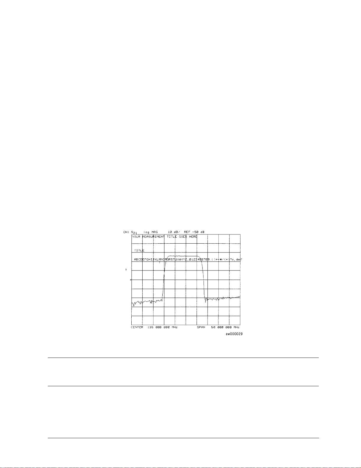
Titling the Active Channel Display

1. Press Display, MORE, TITLE to access the title menu.

Making Measuremen ts

Using Display Functions

2. Press

ERASE TITLE and enter the title you want for your measurement display.

• If you have a DIN keyboard attached to the analyzer, type the title you want from the
keyboard. Then press

ENTER to enter the title into the analyzer. You can enter a title

that has a maximum of 50 characters. (For more information on using a keyboard with
the analyzer, refer to the “Options and Accessories” chapter in the reference guide.)

• If you do not have a DIN keyboard attached to the analyzer, enter the title from the
analyzer front panel.

a. Turn the front panel knob to move the arrow pointer to the first character of the

title.

b. Press

SELECT LETTER.

c. Repeat the previous two steps to enter the rest of the characters in your title. You

can enter a title that has a maximum of 50 characters.

d. Press

DONE, to complete the title entry.

Figure 2-1. Example of a Display Title

CAUTION The NEWLINE, and FORMFEED, keys are not intended for creating display titles.

Those keys are for creating commands to send to peripherals during a sequence
program.

2-5

Making Measurements
Using Display Functions

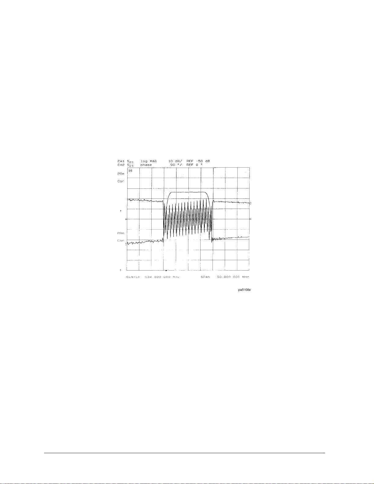
Viewing Both Primary Measurement Channels

In some cases, you may want to view more than one measured parameter at a time.
Simultaneous gain and phase measurements, for example, are useful in evaluating stability
in negative feedback amplifiers. You can easily make such measurements using the dual
channel display.

1. To see channels 1 and 2 in the same grid, press:

Display, DUAL | QUAD SETUP

set DUAL CHAN on OFF to ON, and SPLIT DISP to 1X

Figure 2-2. Example of Viewing Channel 1 and 2 Simultaneously

2. To view the measurements on separate graticules, press: Set

SPLIT DISP to 2X. The

analyzer shows channel 1 on the upper half of the display and channel 2 on the lower half
of the display. The analyzer defaults to measuring O/O on channel 1 and channel 2.

2-6

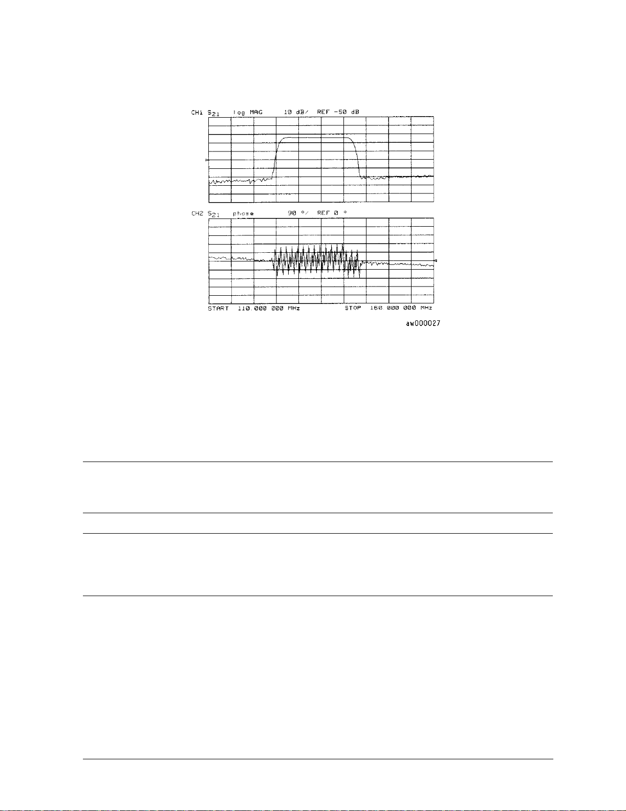
Figure 2-3. Example Dual Channel with Split Display On

Making Measuremen ts

Using Display Functions

3. To return to a single-graticule display, press:

SPLIT DISPLAY 1X.

Dual Channel Mode with Decoupled Stimulus

The stimulus functions of the two channels can be controlled independently using

CH ON off

for each channel using

Fctn

in the sweep setup menu. In addition, the markers can be controlled independently

MARKERS: UNCOUPLED in the marker mode menu, under the Marker

key.

COUPLED

NOTE For dual channel, if channels are uncoupled and you have full 2-port

calibrations on both channels, you will not be able to select a non-ratioed
measurement. For example, you can measure S21 or B/R, but not input B.

NOTE Auxiliary channels 3 and 4 are permanently coupled by stimulus to primary

channels 1 and 2, respectively. Decoupling the primary channels’ stimulus from
each other does not affect the stimulus coupling between the auxiliar y channels
and their primary channels.

Dual Channel Mode with Decoupled Channel Power

By decoupling the channel power or port power and using the dual channel mode, you can
simultaneously view two measurements (or two sets of measurements, if both auxiliary
channels are enabled) having different power levels.

However, there are two configurations that will not sweep continuously.

1. For analyzers with source attenuators, with channel 1 having one attenuation value and
channel 2 set to a different attenuation value, then continuous sweep is disabled to avoid

2-7

Making Measurements
Using Display Functions

wear on the attenuator. A similar situation where this occurs is when a 2-port cal is active
and the port 1 attenuation value is not equal to the port 2 attenuation value. Since one
attenuator is used for both measurements, this would cause the attenuator to
continuously switch power ranges, so continuous sweep is not allowed.

2. Channel 1 is driving one test port and channel 2 is driving the other test port. This would
cause the test port transfer switch to continually cycle. The instrument will not allow the
transfer switch or attenuator to continuously switch ranges in order to update these
measurements without the direct intervention of the operator.

If one of these conditions exist, the test set hold mode will engage, and the status notation
tsH will appear on the left side of the screen. The hold mode leaves the measurement
function in only one of the two measurements. To update both measurement setups, press

Sweep Setup, MEASURE RESTART.

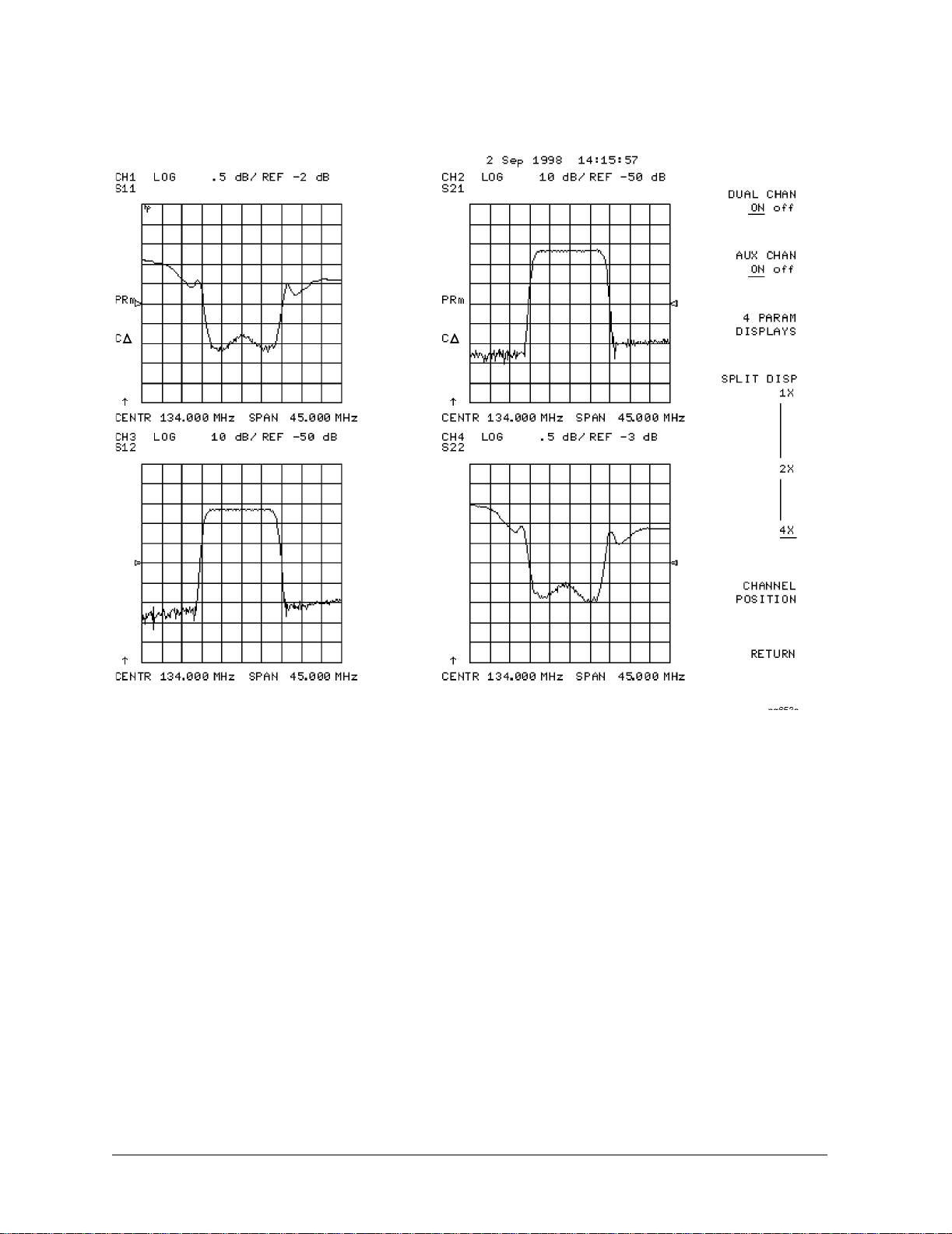
Viewing Four Measurement Channels

Four measurement channels can be viewed simultaneously by enabling auxiliary channels 3
and 4. Although independent of other channels in most variables, channels 3 and 4 are
permanently coupled to channels 1 and 2 respectively by stimulus. That is, if channel 1 is set
for a center frequency of 200 MHz and a span of 50 MHz, channel 3 will have the same
stimulus values.

NOTE Channels 1 and 2 are referred to as primary channels and channels 3 and 4 are

referred to as auxiliary channels.

Channel 3 or 4 are activated when the Chan 3 or Chan 4 keys are pressed. Alternatively, you
can enable the auxiliary channels by setting
active, pressing

AUX CHAN, to ON enables channel 3 and its trace appears on the display.

AUX CHAN to ON. For example, if channel 1 is

Channel 4 is similarly enabled and viewed when channel 2 is active.

1. Press

Format to select the type of display of the data. This example uses the log mag

format.

2. If channel 1 is not active, make it active by pressing

Chan 1.

3. Press Display, DUAL | QUAD SETUP, set DUAL CHAN, to ON, set AUX CHAN, to ON, and set

SPLIT DISP, to 4X.

The display will appear as shown in Figure 2-4 on page 2-9. Channel 1 is in the upper-left
quadrant of the display, channel 2 is in the upper-right quadrant, and channel 3 is in the
lower half of the display.

2-8

Figure 2-4. Three-Channel Display

Making Measuremen ts

Using Display Functions

4. Press Chan 4 (or press

Chan 2, set AUX CHAN, to ON).

This enables channel 4 and the screen now displays four separate grids as shown in

Figure 2-5 on page 2-10. Channel 4 is in the lower-right quadrant of the screen.

2-9

Making Measurements
Using Display Functions

Figure 2-5. Four-Channel Display

5. Press

Chan 4.

Observe that the amber LED adjacent to the Chan 4 key is lit and the CH4 indicator on the
display has a box around it. This indicates that channel 4 is now active and can be
configured.

6. Press

Marker, MARKER 1, MARKER 2.

Markers 1 and 2 appear on all four channel traces. Rotating the front panel control knob
moves marker 2 on all four channel traces. Note that the active function, in this case the
marker frequency, is the same color and in the same grid as the active channel (channel

4).

7. Press

Chan 3.

Observe that the amber LED adjacent to the Chan 3 key is lit. This indicates that channel 3
is now active and can be configured.

8. Rotate the front panel control knob and notice that marker 2 still moves on all four
channel traces.

2-10

Making Measuremen ts

Using Display Functions

9. To independently control the channel markers:

Marker Fctn, MORE, MARKER MODE MENU, set MARKERS: to UNCOUPLED.

Press

Rotate the front panel control knob. Marker 2 moves only on the channel 3 trace.

Once made active, a channel can be configured independently of the other channels in most
variables except stimulus. For example, once channel 3 is active, you can change its format to
a Smith chart by pressing

Format, SMITH CHART.

Customizing the Four-Channel Display

When one or both auxiliary channels are enabled, DUAL CHAN on OFF, and SPLIT DISP 1X 2X

4X,

interact to produce different display configurations according to Table 2-2.

Table 2-2. Customizing the Display

Split Display Dual Channel Aux Channels

On

1X Don't Care Don't Care 1

1X/2X/4X Off None

2X/4X Off 3 or 4 2

2X On Don't Care

4X On 3 or 4 3

4X On Both on 4

Number of
Graticules

Channel Position Softkey

CHANNEL POSITION, gives you options for arranging the display of the channels. Press
Display, DUAL|QUAD SETUP, to use CHANNEL POSITION.

CHANNEL POSITION,
CHANNEL POSITION, gives you two choices for a two-graticule display:

works with SPLIT DISP 1X 2X 4X. When SPLIT DISP 2X, is selected,

• Channels 1 and 2 overlaid in the top graticule, and channels 3 and 4 are overlaid in the
bottom graticule.

• Channels 1 and 3 are overlaid in the top graticule, and channels 2 and 4 are overlaid in
the bottom graticule.

When

SPLIT DISP 4X, is selected, CHANNEL POSITION, gives you two choices for a

four-graticule display:

• Channels 1 and 2 are in separate graticules in the upper half of the display, channels 3
and 4 are in separate graticules in the lower half of the display.

• Channels 1 and 3 are in the upper half of the display, channels 2 and 4 are in the lower
half of the display.

2-11

Making Measurements
Using Display Functions

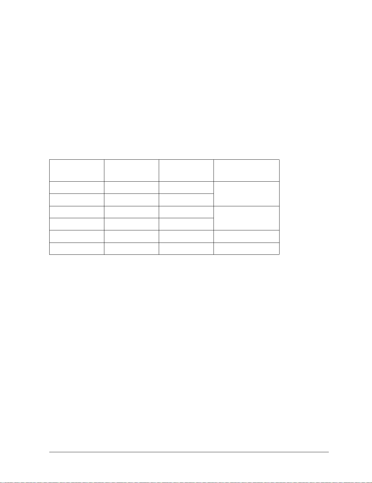
4 Param Displays Softkey

4 PARAM DISPLAYS, menu does two things:

The

• provides a quick way to set up a four-parameter display

• gives information for using softkeys in the

Figure 2-6 shows the first

softkeys

SETUP A, through SETUP F . SETUP A is a four-parameter display where each channel

4 PARAM DISPLAYS, screen. Six setup options are described with

Display, menu

is displayed on its own grid. Pressing SETUP A immediately produces a four-grid,
four-parameter display.

SETUP B, is also a four-parameter display, except that channel 1 and

channel 2 are overlaid on the upper grid and channel 3 and channel 4 are overlaid on the
lower grid. The other setup softkeys operate similarly. Notice that setups D and F produce
displays which include Smith charts.

Pressing

TUTORIAL, opens a screen which lists the order of keystrokes you would have to

enter in order to create some of the setups without using one of the setup softkeys. The
keystroke entries are listed (from top to bottom) beneath each setup and are color-coded to
show the relationship between the keys and the channels. For example, beneath the four-grid
display, [CHAN 1] and [MEAS] S11 are shown in yellow. Notice that in the four-grid graphic,
Ch1 is also yellow, indicating that the keys in yellow apply to channel 1.

Pressing

MORE HELP, opens a screen which lists the hardkeys and softkeys associated with

the auxiliary channels and setting up multiple-channel, multiple-grid displays. Next to each
key is a description of its function.

Figure 2-6. 4 Param Displays Menu

2-12

Making Measuremen ts

Using Display Functions

Using Memory Traces and Memory Math Functions

The analyzer has four available memory traces, one per channel. Memory trace 1 and
memory trace 2 can be used with either channel 1 or channel 2. Memory trace 3 is only
associated with channel 3, and memory trace 4 is only associated with channel 4.

Memory traces can be saved with instrument states: one memory trace can be saved per
channel for each saved instrument state. There are up to 31 save/recall registers available, so
the total number of memory traces that can be present is 128 including the four active for the
current instrument state. The memory data is stored as full precision, complex data. Memor y
traces must be displayed in order to be saved with instrument states.

Additional data can be stored onto 3.5-inch floppy disks using the front panel disk drive.

NOTE You may not be able to store 31 instrument states if they include a large amount

of calibration data. The calibration data contributes considerably to the size of
the instrument state file and therefore the available memory may be full prior
to filling all 31 registers. “Memory Allocation” on page 8-13 in the Reference.

The following trace math operations are implemented:

Table 2-3.

DATA/MEM MEM1/MEM2
DATA-MEM MEM1-MEM2

DATA∗MEM
DATA+MEM MEM2/MEM1

MEM/DATA MEM2-MEM1

MEM-DATA

MEM1∗MEM2

Memory traces are saved and recalled and trace math is performed immediately after
error-correction. This means that any data processing done after error-correction, including
parameter conversion, scaling, and so forth, can be performed on the memory trace. You can
also use trace math as a simple means of error-correction, although that is not its main
purpose.

All data processing operations that occur after trace math, except smoothing is identical for
the data trace and the memory trace. If smoothing is on when a memory trace is saved, this
state is maintained regardless of the data trace smoothing. If a memory trace is saved with
smoothing on, this feature can be turned on or off in the memory-only display mode.

The actual memory for storing a memory trace is allocated only as needed. The memory trace
is cleared on instrument preset, power on, or instrument state recall.

If sweep mode or sweep range is different between the data and memory traces, trace math
is allowed, and no warning message is displayed. If the number of points in the two traces is

2-13

Making Measurements
Using Display Functions

different, the memory trace is not displayed nor rescaled. However, if the number of points
for the data trace is changed back to the number of points in the memory, the memory trace
can then be displayed.

If trace math or display memory is requested and no memory trace exists, the message
CAUTION: NO VALID MEMORY TRACE is displayed.

To Save a Data Trace to the Display Memory

Press

Display, DAT A→MEMORY, to store the current active measurement data in the memory

of the active channel. The data trace is now also the memory trace. You can use a memory
trace for subsequent math manipulations.

To View the Measurement Data and Memory Trace

The analyzer default setting shows you the current measurement data for the active channel.

1. To view a data trace that you have already stored to the active channel memory, press:

Display, MEMORY

This is the only memory display mode where you can change the smoothing of the
memory trace.

2. To view both the memory trace and the current measurement data trace, press:

Display, DATA and MEMORY

To Perform a Math Function

1. You must have already stored a data trace to the active channel memory, as described in

“To Save a Data Trace to the Display Memory” on page 2-14.

2. Press

Display, MATH:DAT A/MEM to divide the data by the memory.

3. To perform other math functions on the measurement data and memory, use the menu
under the

MATH:DAT A/MEM key.

Blanking the Display

Pressing Display, MORE, ADJUST DISPLAY, BLANK DISPLAY switches off the analyzer display
while leaving the instrument in its current measurement state. This feature may be helpful in
prolonging the life of the LCD in applications where the analyzer is left unattended (such as
in an automated test system). Turning the front panel knob or pressing any front panel key
will restore normal display operation.

Pressing Display, FREQUENCY BLANK will blank the displayed frequency notation for
security purposes. The frequency labels cannot be restored except by instrument preset or
turning the power off and then on.

2-14

Adjusting the Colors of the Display

Setting Display Intensity

Making Measuremen ts

Using Display Functions

To adjust the intensity of the display, press
rotate the front panel knob, use the (

up,) (down,) keys, or use the numerical keypad to set the

Display, MORE, ADJUST DISPLAY, INTENSITY, and

intensity value between 50 and 100 percent. Lowering the intensity may prolong the life of
the LCD.

Setting Default Colors

To set all the display elements to the factory-defined default colors, press DISPLAY, MORE
ADJUST DISPLAY,

DEFAULT COLORS.

NOTE Preset, does not reset or change colors to the default color values. However,

cycling power to the instrument will reset the colors to the default color values.

The Modify Colors Menu

MODIFY COLORS softkey within the adjust display menu provides access to the modify

The
colors menu.

The modify colors menu allows you to adjust the colors on your analyzer's display. The
default colors in this instrument were chosen to maximize your ability to discern the
difference between the channel colors, and to comfortably and effectively view the colors.
Each channel’s memory trace color was chosen because the color is similar to the channels
data trace color. This allows easy association between the data trace and the memory trace
for each channel.

You may choose to change the default colors to suit environmental needs, individual
preferences, or to accommodate color deficient vision. You can use any of the available colors
for any of the display elements listed:

CH1 DATA/LIMIT LN CH3 DATA/LIMIT LN
CH1 MEM CH3 MEM
CH2 DATA/LIMIT LN CH4 DATA/LIMIT LN
CH2 MEM CH4 MEM
GRATICULE REF LINE
TEXT WARNING
RIPPLE LIM LINES

To change the color of a display element, press the softkey for that element (such as

). Then press TINT and turn the analyzer front panel knob; use the step keys or the

DATA

CH1

numeric keypad, until the desired color appears.

2-15

Making Measurements
Using Display Functions

NOTE Maximum viewing with the LCD display is achieved when primary colors or a

combination of them are selected at full brightness (100%). Table 2-4 lists the
recommended colors and their corresponding tint numbers.

Table 2-4. Display Colors with Maximum Viewing Angle

Display Color Tint Brightness Color

Red 0 100 100

Yellow 17 100 100

Green 33 100 100

Cyan 50 100 100

Blue 67 100 100

Magenta 83 100 100

White N/A 100 0

Color is comprised of three parameters:

• Tint: The continuum of hues on the color wheel, ranging from red, through green and
blue, and back to red.

• Brightness: A measure of the brightness of the color.

• Color: The degree of whiteness of the color. A scale from white to pure color.

The most frequently occurring color deficiency is the inability to distinguish red, yellow, and
green from one another. Confusion between these colors can usually be eliminated by
increasing the brightness between the colors. To accomplish this, press the

BRIGHTNESS

softkey and turn the analyzer front panel knob. If additional adjustment is needed, vary the
degree of whiteness of the color. To accomplish this, press the

COLOR, softkey and turn the

analyzer front panel knob.

NOTE Color changes and adjustments remain in effect until changed again in these

menus or the analyzer is powered off and then on again. Cycling the power
changes all color adjustments to default values. Once the colors are saved,
pressing the Preset key does not affect the color selections.

Saving Modified Colors

To save a modified color set, press

Display , MORE, ADJUST DISPLAY, SAVE COLORS. Modified

colors are not part of a saved instrument state and are lost unless saved using these softkeys.
Once modified colors are saved, they will be the colors applied until you press

Preset.

Recalling Modified Colors

To recall the previously saved color set, press

2-16

RECALL COLORS.

Making Measuremen ts

Using Markers

Using Markers

The Marker, key displays a movable active marker on the screen and provides access to a
series of menus to control up to five display markers for each channel. By using markers, you
can obtain numerical readings of measured values. Markers also provide capabilities for
reducing measurement time by changing stimulus parameters, searching the trace for
specific values, or statistically analyzing part or all of the trace.

Markers have a stimulus value (the x-axis value in a Cartesian format) and a response value
(the y-axis value in a Cartesian format). In polar format, the second part of a complex data
pair is also provided as an auxiliary response value. In Smith chart format, the real and
imaginary rectangle are both displayed, and the effective capacitance or inductance of the
imaginary part is also displayed. When a marker is activated and no other function is active,
its stimulus value is displayed in the active entry area and can be controlled with the knob,
the step keys, or the numeric keypad. The active marker can be moved to any point on the
trace, and its response and stimulus values are displayed at the top right corner of the
graticule for each displayed channel, in units appropriate to the display format. The
displayed marker response values are valid even when the measured data is above or below
the range displayed on the graticule.

• If you activate both data and memory traces, the marker values apply to the data trace.

• If you activate only the memory trace, the marker values apply to the memory trace.

• If you activate a memory math function, the marker values apply to the trace resulting
from the memory math function.

Marker values are normally continuous: that is, they are interpolated between measured
points. They can also be set to read only discrete measured points. Markers normally have
the same stimulus values for all channels, or they can be uncoupled so that each channel has
independent markers, regardless of whether stimulus values are coupled or dual channel
display is on.

To Use Continuous and Discrete Markers

The analyzer can either place markers on discrete measured points, or move the markers
continuously along a trace by interpolating the data value between measured points.

• Press

Marker Fctn, MORE, MARKER MODE MENU, and select one of the following choices:

—Choose

point on the trace, by interpolating between measured points. This default mode allows
you to conveniently obtain round numbers for the stimulus value.

—Choose

measured trace points determined by the stimulus settings. This may be the best mode
to use with automated testing, using a computer or test sequencing because the
analyzer does not interpolate between measured points.

MARKERS: CONTINUOUS, if you want the analyzer to place markers at any

MARKERS: DISCRETE, if you want the analyzer to place markers only on

2-17

Making Measurements
Using Markers

NOTE Using MARKERS: DISCRETE, will also affect marker search and positioning

functions when the value entered in a search or positioning function does not
exist as a measurement point. The marker will be positioned to the closest
adjacent point that satisfies the search or positioning value.

To Activate Display Markers

• To switch on marker 1 and make it the active marker, press:

Marker, MARKER 1

The active marker is identified on the analyzer display with the following symbol: ∇

The active marker stimulus value is displayed in the active entry area. You can modify the
stimulus value of the active marker, using the front panel knob or numerical keypad. All of
the marker response and stimulus values are displayed in the upper right corner of the
display.

Figure 2-7. Active Marker Control Example

To switch on the corresponding marker and make it the active marker, press:

MARKER 2 or MARKER 3 or MARKER 4, or MARKER 5

All of the markers, other than the active marker, become inactive and are represented on the

analyzer display as ∆. The active and inactive markers are shown in Figure 2-8.

2-18

Figure 2-8. Active and Inactive Markers Example

Making Measuremen ts

Using Markers

• To switch off all of the markers, press

ALL OFF.

To Move Marker Information Off the Grids

If marker information obscures the display traces, you can turn off the softkey menu and
move the marker information off the display traces and into the softkey menu area. Pressing

the backspace key ⇐

alternately hides and restores the current softkey menu. The softkey menu is also restored
when you press any softkey or a hardkey which leads to a menu. The following procedure
shows how you can view the marker information in the softkey area.

1. Set up a four-graticule display as described in "Viewing Four Measurement Channels" on

page 1-18.

2. Activate four markers by pressing

NOTE Observe that the markers appear on all of the grids. To activate markers on

individual grids, press Marker Fctn, MORE, MARKER MODE MENU, and set

MARKERS:, to UNCOUPLED. Then, activate the channel in which you wish to

have markers, press Marker then select the markers for that channel.

3. Turn off the softkey menu and move the marker information off the grids by pressing ⇐.

The display will be similar to Figure 2-9.

, performs this function. This is a toggle function. Pressing ⇐,

Marker, 1, 2, 3, 4.

2-19

Making Measurements
Using Markers

Figure 2-9. Marker Information Moved into the Softkey Menu Area

pg654e

4. Restore the softkey menu and move the marker information back onto the graticules:

Press ⇐

.

The display will be similar to Figure 2-10.

2-20

Figure 2-10. Marker Information on the Graticules

Making Measuremen ts

Using Markers

pg655e

You can also restore the softkey menu by pressing a hardkey which opens a menu (such as

Meas) or pressing a softkey.

To Use Delta (∆) Markers

This is a relative mode, where the marker values show the position of the active marker
relative to the delta reference marker. You can switch on the delta mode by defining one of
the five markers as the delta reference.

1. Press

2. To move marker 1 to any point that you want to reference:

3. Press

Marker, ∆ MODE MENU, ∆ REF=1, to make marker 1 a reference marker.

•Turn the front panel knob.

OR

• Enter the frequency value (relative to the reference marker) on the numeric keypad.

Marker, MARKER 2, and move marker 2 to any position that you want to measure in

reference to marker 1.

2-21

Making Measurements
Using Markers

Figure 2-11. Marker 1 as the Reference Marker Example

4. To change the reference marker to marker 2, press:

∆ MODE MENU, ∆ REF=2

To Activate a Fixed Marker

When a reference marker is fixed, it does not rely on a current trace to maintain its fixed
position. This is convenient when comparing two different measurement conditions. To
activate a fixed marker on the analyzer, press

Marker zero puts a fixed reference at the current position of the active marker.

To change to a Delta Marker to a fixed reference marker, press

∆REF=∆FIXED MKR.

Using the MKR ZERO Key to Activate a Fixed Reference Marker

Marker zero enters the position of the active marker as the ∆ reference position.

Alternatively, you can specify the fixed point with
canceled by switching delta mode off.

1. To place marker 1 at a point that you would like to reference, press:

Marker, and turn the front panel knob, or enter a value from the front panel keypad.

2. To measure values along the measurement data trace, relative to the reference point that
you set in the previous step, press:

MKR ZERO, and turn the front panel knob, or enter a value from the front panel keypad.

Marker, MKR ZERO.

Marker, ∆ MODE MENU,

FIXED MKR POSITION. Marker zero is

3. To move the reference position, press:

∆MODE MENU, FIXED MKR POSITION, FIXED MKR STIMULUS, and turn the front panel

knob, or enter a value from the front panel keypad.

2-22

Figure 2-12. Example of a Fixed Reference Marker Using MKR ZERO

Making Measuremen ts

Using Markers

Using the

∆REF=∆FIXED MKR, Key to Activate a Fixed Reference Marker

1. To set the frequency value of a fixed marker that appears on the analyzer display, press:

Marker, ∆MODE MENU, ∆REF=∆FIXED MKR, ∆MODE MENU, FIXED MKR POSITION, FIXED
MKR STIMULUS,

and turn the front panel knob, or enter a value from the front panel

keypad.

The marker is shown on the display as a small delta (∆), smaller than the inactive marker

triangles.

2. To set the response value (dB) of a fixed marker, press:

FIXED MKR VALUE, and turn the front panel knob, or enter a value from the front panel

keypad.

In a Cartesian format, the setting is the y-axis value. In polar or Smith chart format, with
a magnitude/phase marker, a real/imaginary marker, an R+jX marker, or a G+jB marker,
the setting applies to the first part of the complex data pair. (Fixed marker response
values are always uncoupled in the two channels.)

3. To set the auxiliary response value of a fixed marker when you are viewing a polar or
Smith format, press:

FIXED MKR AUX VALUE, and turn the front panel knob, or enter a value from the front

panel keypad.

This value is the second part of complex data pair, and applies to a magnitude/phase
marker, a real/imaginary marker, an R+jX marker, or a G+jB marker. (Fixed marker
auxiliary response values are always uncoupled in the two channels.)

2-23

Making Measurements
Using Markers

Figure 2-13. Example of a Fixed Reference Marker Using (∆)REF=(∆)FIXED MKR

To Couple and Uncouple Display Markers

At a preset state, the markers have the same stimulus values on each channel, but they can
be uncoupled so that each channel has independent markers.

Press

• Choose

Marker Fctn, MORE, MARKER MODE MENU, and select from the following keys:

MARKERS: COUPLED, if you want the analyzer to couple the marker stimulus

values for the display channels.

• Choose

MARKERS: UNCOUPLED, if you want the analyzer to uncouple the marker

stimulus values for the display channels. This allows you to control the marker stimulus
values independently for each channel.

Figure 2-14. Example of Coupled and Uncoupled Markers

2-24

Making Measuremen ts

Using Markers

To Use Polar Format Markers

The analyzer can display the marker value as magnitude and phase, or as a real/imaginary
pair: LIN MKR, gives linear magnitude and phase, LOG MKR, gives log magnitude and phase,

Re/Im, gives the real value first, then the imaginary value.

You can use these markers only when you are viewing a polar display format. (The format is
available from the

NOTE For greater accuracy when using markers in the polar format, it is

1. To access the polar markers, press:

Format, POLAR, Marker Fctn, MORE, MARKER MODE MENU, POLAR MKR MENU

2. Select the type of polar marker you want from the following choices:

Format, key.)

recommended to activate the discrete marker mode. Press

MKR MODE MENU, MARKERS:DISCRETE.

Marker Fctn, MORE,

•Choose

LIN MKR, if you want to view the magnitude and the phase of the active marker.

The magnitude values appear in units and the phase values appear in degrees.

•Choose

LOG MKR, if you want to view the logarithmic magnitude and the phase of the

active marker. The magnitude values appear in dB and the phase values appear in
degrees.

•Choose

Re/Im MKR, if you want to view the real and imaginary pair, where the complex

data is separated into its real part and imaginary part. The analyzer shows the real

part as the first marker value (M cos Θ), and the second value is the imaginary part (M
sin Θ, where M = magnitude).

Figure 2-15. Example of a Log Marker in Polar Format

2-25

Making Measurements
Using Markers

To Use Smith Chart Markers

To avoid displaying marker data interpolated between measured points when using markers
in the Smith chart format, activate the discrete marker mode. Press

MODE MENU,

interpolate between points.)

MARKERS:DISCRETE. (Discrete markers will display only measured data and do not

To use Smith chart format:

Marker Fctn, MORE, MKR

1. Press

Format, SMITH CHART.

2. Press Marker Fctn, MORE, MARKER MODE MENU, SMITH MKR MENU, and turn the front

panel knob, or enter a value from the front panel keypad to read the resistive and reactive
components of the complex impedance at any point along the trace. This is the default
Smith chart marker.

The marker annotation tells that the complex impedance is capacitive in the bottom half
of the Smith chart display and is inductive in the top half of the display.

•Choose

LIN MKR, if you want the analyzer to show the linear magnitude and the phase

of the reflection coefficient at the marker.

•Choose

LOG MKR, if you want the analyzer to show the logarithmic magnitude and the

phase of the ref lection coefficient at the active marker. This is useful as a fast method
of obtaining a reading of the log magnitude value without changing to log magnitude
format.

•Choose

Re/Im MKR, if you want the analyzer to show the values of the reflection

coefficient at the marker as a real and imaginary pair.

•Choose

R+jX MKR, to show the real and imaginary parts of the device impedance (the

series resistance and reactance, in ohms) at the marker. Also shown is the equivalent
series inductance or capacitance.

•Choose

G+jB MKR, to show the complex admittance values of the active marker in

rectangular form. The active marker values are displayed in terms of conductance (in
Siemens), susceptance, and equivalent parallel circuit capacitance or inductance.
Siemens are the international unit of admittance and are equivalent to mhos (the
inverse of ohms).

2-26

Figure 2-16. Example of Impedance Smith Chart Markers

To Set Measurement Parameters Using Markers

Making Measuremen ts

Using Markers

The analyzer allows you to set measurement parameters with the markers, without going
through the usual key sequence. You can change certain stimulus and response parameters
to make them equal to the current active marker value.

Setting the Start Frequency

1. Press

Marker Fctn, and turn the front panel knob, or enter a value from the front panel

keypad to position the marker at the value that you want for the start frequency.

2. Press

MARKER→START, to change the start frequency value to the value of the active

marker.

Figure 2-17. Example of Setting the Start Frequency Using a Marker

2-27

Making Measurements
Using Markers

Setting the Stop Frequency

1. Press

Marker Fctn, and turn the front panel knob, or enter a value from the front panel

keypad to position the marker at the value that you want for the stop frequency.

2. Press

MARKER→STOP, to change the stop frequency value to the value of the active

marker.

Figure 2-18. Example of Setting the Stop Frequency Using a Marker

Setting the Center Frequency

1. Press

Marker Fctn, and turn the front panel knob, or enter a value from the front panel

keypad to position the marker at the value that you want for the center frequency.

2. Press

MARKER→CENTER, to change the center frequency value to the value of the active

marker.

Figure 2-19. Example of Setting the Center Frequency Using a Marker

2-28

Making Measuremen ts

Using Markers

Setting the Frequency Span

You can set the span equal to the spacing between two markers. If you set the center
frequency before you set the frequency span, you will have a better view of the area of
interest.

1. Press

Marker, ∆MODE MENU, ∆REF=1, MARKER 2.

2. Turn the front panel knob, or enter a value from the front panel keypad to position the
markers where you want the frequency span.

Iterate between marker 1 and marker 2 by pressing

MARKER 1, and MARKER 2,

respectively, and turning the front panel knob or entering values from the front panel
keypad to position the markers around the center frequency. When finished positioning
the markers, make sure that marker 2 is selected as the active marker.

NOTE Step 2 can also be performed using MKR ZERO, and MARKER 1. However, when

using this method, it will not be possible to iterate between marker zero and
marker 1.

3. Press Marker Fctn, MARKER→SPAN, to change the frequency span to the range between

marker 1 and marker 2.

Figure 2-20. Example of Setting the Frequency Span Using Marker

Setting the Display Reference Value

1. Press

Marker Fctn, and turn the front panel knob, or enter a value from the front panel

keypad to position the marker at the value that you want for the analyzer display
reference value.

2. Press

MARKER→REFERENCE, to change the reference value to the value of the active

marker.

2-29

Making Measurements
Using Markers

Figure 2-21. Example of Setting the Reference Value Using a Marker

Setting the Electrical Delay

This feature adds phase delay to a variation in phase versus frequency, therefore it is only
applicable for ratioed inputs.

1. Press

Format, PHASE.

2. Press Marker Fctn, and turn the front panel knob, or enter a value from the front panel

keypad to position the marker at a point of interest.

3. Press

MARKER→DELAY, to automatically add or subtract enough line length to the

receiver input to compensate for the phase slope at the active marker position. This
effectively flattens the phase trace around the active marker. You can use this to measure
the electrical length or deviation from linear phase.

Additional electrical delay adjustments are required on devices without constant group
delay over the measured frequency span.

2-30

Figure 2-22. Example of Setting the Electrical Delay Using a Marker

Setting the CW Frequency

Making Measuremen ts

Using Markers

1. To place a marker at the desired CW frequency, press:

Marker, and either turn the front panel knob or enter the value, followed by a unit

terminator.

2. Press

Seq, SPECIAL FUNCTIONS, MKR→CW.

You can use this function to set the marker to a gain peak in an amplifier. After pressing

MKR→CW FREQ, activate a CW frequency power sweep to look at the gain compression

with increasing input power.

2-31

Making Measurements
Using Markers

To Search for a Specific Amplitude

These functions place the marker at an amplitude-related point on the trace. If you switch on
tracking, the analyzer searches every new trace for the target point.

Searching for the Maximum Amplitude

1. Press

2. Press

Marker Search, to access the marker search menu.
SEARCH: MAX, to move the active marker to the maximum point on the

measurement trace.

Figure 2-23. Example of Searching for the Maximum Amplitude Using a Marker

Searching for the Minimum Amplitude

1. Press

2. Press

Marker Search, to access the marker search menu.
SEARCH: MIN, to move the active marker to the minimum point on the measurement

trace.

2-32

Making Measuremen ts

Figure 2-24. Example of Searching for the Minimum Amplitude Using a Marker

Searching for a Target Amplitude

Using Markers

1. Press

2. Press

Marker Search, to access the marker search menu.
SEARCH: TARGET, to move the active marker to the target point on the

measurement trace.

3. If you want to change the target amplitude value (default is −3 dB), press

TARGET, and

enter the new value from the front panel keypad. You may also press Marker Search,

TARGET VALUE, to enter the new value.

4. If you want to search for multiple responses at the target amplitude value, press

and SEARCH RIGHT.

LEFT,

Figure 2-25. Example of Searching for a Target Amplitude Using a Marker

SEARCH

2-33

Making Measurements
Using Markers

Searching for the 3 dB Bandwidth of a Lowpass Device

The analyzer can search for the 3 dB bandwidth, locating the rolloff on the high side of a
device’s passband.

1. Press

Marker, Marker 1.

2. Move marker 1 to any point that you want to reference:

•Turn the front panel knob.

OR

• Enter the frequency value on the numeric keypad.

5. Press Marker Search, 3 DB BANDWIDTH.

Searching for the Bandwidth and Related Information of a Bandpass Device

The analyzer can automatically calculate and display the bandwidth (BW:), center frequency
(CENT:), Q, and loss of the device under test at the center frequency. (Q stands for “quality
factor,” defined as the ratio of a circuit's resonant frequency to its bandwidth.) These values
are shown in the marker data readout.

1. Press

Marker Search, and SEARCH: MAX, to place the marker near the center of the filter

passband.

2. Press Marker,

3. Press

Marker Fctn, MORE, BANDWIDTH VALUE and enter the amplitude value (default

MKR ZERO, if you want the bandwidth relative to the maximum.

is −3 dB) that defines the passband or reject band.

4. If you want to change the amplitude value (default is −3 dB) that defines the passband or

reject band, press

WIDTH VALUE, and enter the new value from the front panel keypad.

5. Press BANDWIDTH for the analyzer to calculate the center stimulus value, bandwidth,
and the Q of a bandpass or band reject shape on the measurement trace.

Figure 2-26. Example of Searching for the Bandwidth of a Bandpass Device

2-34

Making Measuremen ts

Using Markers

Tracking the Amplitude that You Are Searching

1. Set up an amplitude search by following one of the previous procedures in “To Search for

a Specific Amplitude” on page 2-32.

2. Press

Marker Search, TRACKING ON, to track the specified amplitude search with every

new trace and put the active marker on that point.

When tracking is not activated, the analyzer finds the specified amplitude on the current
sweep and the marker remains at same stimulus value, regardless of changes in the trace
response value with subsequent sweeps.

To Calculate the Statistics of the Measurement Data

This function calculates the mean, st andard deviation, and peak-to-peak values of the section
of the displayed trace between the active marker and the delta reference. If there is no delta
reference, the analyzer calculates the statistics for the entire trace.

1. Move marker 1 to any point that you want to reference:

•Turn the front panel knob.

OR

• Enter the frequency value on the numeric keypad.

2. Press

3. Press

4. Press

Marker, ∆ MODE MENU, ∆ REF=1, to make marker 1 a reference marker.
MARKER 2, and move marker 2 to any position that you want to measure in

reference to marker 1.

Marker Fctn, MORE, MKR MODE MENU, MKR STATS ON, to calculate and view the

mean, standard deviation, and peak-to-peak values of the section of the measurement
data between the active marker and the delta reference marker.

An application for this feature is to find the peak-to-peak value of passband ripple
without searching separately for the maximum and minimum values.

If you are viewing a measurement in the polar or Smith Chart format, the analyzer
calculates the statistics using the first value of the complex pair (magnitude, real part,
resistance, or conductance).

2-35

Making Measurements
Using Markers

Figure 2-27. Example Statistics of Measurement Data

Figure 0-1

2-36

Making Measuremen ts

Using the List Mode to Test a Device

Using the List Mode to Test a Device

When using a list frequency sweep, the analyzer has the ability to sweep arbitrary frequency
segments, each containing a list of frequency points. One major advantage of using list
frequency sweep is that it allows you to measure the minimum number of data points, and
only at the frequencies of interest. This serves to minimize the overall test time. Two
different list frequency sweep modes can be selected:

Stepped List
Mode In this mode, the source steps to each defined frequency point, stopping

while data is taken. This mode eliminates IF delay and allows frequency
segments to overlap. However, the sweep time is substantially slower than
for a continuous sweep with the same number of points.

Swept List
Mode Use this mode for electrical-to-electrical device measurements only. This

mode takes data while sweeping through the defined frequency segments,
increasing throughput by up to 6 times over a stepped sweep. In addition,
this mode allows the test port power and IF bandwidth to be set
independently for each segment that is defined. The frequency segments in
this mode cannot overlap.

The ability to completely customize the frequency sweep while using swept list mode is
useful when setting up a measurement for a device with high dynamic range, like a filter. The
following measurement of a filter illustrates the advantages of using the swept list mode.

• For in-depth information on swept list mode, refer to "Swept List Frequency Sweep (Hz)"

on page 7-22.

Connect the Device Under Test

1. Connect the equipment for a transmission measurement.

2. Set the following measurement parameters:

Meas, ELECTRICAL PARAMETERS, Trans:FWD S21 (B/R)
Center,
Span,

900, M/µ

500, M/µ

2-37

Making Measurements
Using the List Mode to Test a Device

Observe the Characteristics of the Filter

Figure 2-28. Characteristics of a Filter

• Generally, the passband of a filter exhibits low loss. A relatively low incident power may
be needed to avoid overdriving the next stage of the DUT (if that stage contains an
amplifier) or the analyzer receiver.

• Conversely, the stopband of a filter generally exhibits high isolation. To measure this
characteristic, the dynamic range of the system will have to be maximized. This can be
done by increasing the incident power and narrowing the IF bandwidth.

Choose the Measurement Parameters

1. Decide the frequency ranges of the segments that will cover the stopbands and passband
of the filter. For this example, the following ranges will be used:

• Lower stopband: 650 to 880 MHz

• Passband: 880 to 920 MHz

• Upper stopband: 920 to 1150 MHz

2. To set up the swept list measurement, press:

Sweep Setup, SWEEP TYPE MENU, EDIT LIST

2-38

Set Up the Lower Stopband Parameters

3. To set up the segment for the lower stopband, press

ADD

Making Measuremen ts

Using the List Mode to Test a Device

START,
STOP, 880, M/µ
NUMBER of POINTS, 51, x1

650, M/µ

4. To maximize the dynamic range in the stopband (increasing the incident power and
narrowing the IF bandwidth), press

MORE
LIST POWER ON off,
LIST IF BW ON off,
RETURN,

DONE

until ON is selected SEGMENT POWER, 10, x1

until ON is selected SEGMENT IF BW, 1000, x1

Set Up the Passband Parameters

5. To set up the segment for the passband, press

ADD
CENTER,
SPAN, 40, M/µ
STEP SIZE, .2, M/µ

900, M/µ

6. To specify a lower power level and a wider IF bandwidth for the passband, press

MORE
SEGMENT POWER,
SEGMENT IF BW,
RETURN,

DONE

-10, x1

3700, x1

Set Up the Upper Stopband Parameters

7. To set up the segment for the upper stopband, press

ADD
START,
STOP, 1150, M/µ
NUMBER of POINTS, 51, x1

920, M/µ

2-39

Making Measurements
Using the List Mode to Test a Device

8. To maximize the dynamic range in the stopband (increasing the incident power and
narrowing the IF bandwidth), press:

MORE
SEGMENT POWER,
SEGMENT IF BW,
RETURN,

DONE

10, x1

300, x1

9. Press DONE, LIST FREQ [SWEPT].

Calibrate and Measure

1. Remove the DUT and perform a full two-port calibration. Refer to Chapter 4, “Calibrating

for Increased Measurement Accuracy”

2. With the thru connected, set the scale to autoscale to observe the benefits of using swept
list mode.

• The segments used to measure the stopbands have less noise, thus maximizing

dynamic range within the stopband frequencies.

• The segment used to measure the passband has been set up for faster sweep speed

with more measurement points.

Figure 2-29. Calibrated Swept List Thru Measurement

3. Reconnect the filter and adjust the scale to compare results with the first filter
measurement that used a linear sweep.

In Figure 2-29, notice that the noise level has decreased over 10 dB, confirming that the
noise reduction techniques in the stopbands were successful. Also, notice that the
stopband noise in the third segment is slightly lower than in the first segment. This is due
to the narrower IF bandwidth of the third segment (300 Hz).

2-40

Making Measuremen ts

Using the List Mode to Test a Device

Figure 2-30. Filter Measurements Using Linear Sweep and Swept List Mode

Using Linear Sweep

(Power: 0 dBm/IF BW: 3700 Hz)

Using Swept List Mode

2-41

Making Measurements
Using Limit Lines to Test a Device

Using Limit Lines to Test a Device

Limit testing is a measurement technique that compares measurement data to constraints
that you define. Depending on the results of this comparison, the analyzer will indicate if
your device either passes or fails the test.

Limit testing is implemented by creating individual flat, sloping, and single-point limit lines
on the analyzer display. When combined, these lines can represent the performance
parameters for your device under test. The limit lines created on each measurement channel
are independent of each other.

This example measurement shows you how to test a bandpass filter using the following
procedures:

• creating flat limit lines

• creating sloping limit lines

• creating single point limit lines

• editing limit segments

• running a limit test

Setting Up the Measurement Parameters

1. Set up the test equipment for a transmission measurement.

2. Press

Preset, and choose the measurement settings. For this example the measurement

settings are as follows:

Meas, ELECTRICAL PARAMETERS, Trans:FWD S21 (B/R)

•

• Center, 134, M/µ

Span, 50, M/µ

•

Scale Ref, AUTO SCALE

•

You may also want to select settings for the number of data points, power, averaging, and
IF bandwidth.

4. Substitute a thru for the device and perform a response calibration by pressing:

Cal, CALIBRATE MENU, RESPONSE, THRU, DONE: RESPONSE

5. Reconnect your test device.

Creating Flat Limit Lines

In this example procedure, the following flat limit line values are set:

Frequency Range Power Range

127 MHz to 140 MHz −27 dB to −21 dB
100 MHz to 123 MHz −200 dB to −65 dB
146 MHz to 160 MHz −200 dB to −65 dB

2-42

Making Measuremen ts

Using Limit Lines to Test a Device

NOTE The minimum value for measured data is −200 dB.

1. To access the limits menu and activate the limit lines, press:

System, LIMIT MENU, LIMIT LINE, LIMIT LINE ON, EDIT LIMIT LINE, CLEAR LIST, YES

2. To create a new limit line, press:

ADD

The analyzer generates a new segment that appears on the center of the display.

3. To specify the limit's stimulus value, test limits (upper and lower), and the limit type,
press:

STIMULUS VALUE, 127, M/µ
UPPER LIMIT, -21, x1
LOWER LIMI T, -27, x1, DONE

NOTE You could also set the upper and lower limits by using the MIDDLE VALUE, and

DELTA LIMITS keys. To use these keys for the entry, press:
MIDDLE VALUE, -24, x1, DELTA LIMITS, 3, x1

This would correspond to a test specification of −24 ±3 dB.

4. To define the limit as a flat line, press:

LIMIT TYPE, FLAT LINE, RETURN

5. To terminate the f lat line segment by establishing a single point limit, press:

ADD, STIMULUS VALUE, 140, M/µ, DONE
LIMIT TYPE, SINGLE POINT, RETURN

Figure 2-31 shows the flat limit lines that you have just created with the following

parameters:

• stimulus from 127 MHz to 140 MHz

• upper limit of −21 dB

• lower limit of −27 dB

2-43

Making Measurements
Using Limit Lines to Test a Device

Figure 2-31. Example Flat Limit Line

• To create a limit line that tests the low side of the filter, press:

ADD
STIMULUS VALUE,

UPPER LIMIT, −65, x1
LOWE R LIMIT,
DONE

LIMIT TYPE,
ADD
STIMULUS VALUE,
DONE
LIMIT TYPE,

FLAT LINE, RETURN

SINGLE POINT, RETURN

100, M/µ

-200, x1

123, M/µ

• To create a limit line that tests the high side of the bandpass filter, press:

ADD
STIMULUS VALUE,

UPPER LIMIT, −65, x1
LOWE R LIMIT,
DONE

146, M/µ

−200, x1

2-44

LIMIT TYPE,
ADD
STIMULUS VALUE,
DONE
LIMIT TYPE,

FLAT LINE, RETURN

SINGLE POINT, RETURN

160, M/µ

Figure 2-32. Example Flat Limit Lines

Creating a Sloping Limit Line

Making Measuremen ts

Using Limit Lines to Test a Device

This example procedure shows you how to make limits that test the shape factor of a SAW
filter. The following limits are set:

Frequency Range Power Range

123 MHz to 125 MHz −65 dB to −26 dB
144 MHz to 146 MHz −26 dB to −65 dB

1. To access the limits menu and activate the limit lines, press:

System, LIMIT MENU, LIMIT LINE, LIMIT LINE ON, EDIT LIMIT LINE, CLEAR LIST, YES

2. To establish the start frequency and limits for a sloping limit line that tests the low side of
the filter, press:

ADD, STIMULUS VALUE, 123, M/µ
UPPER LIMIT, −65, x1, LOWER LIMIT, −200, x1
DONE, LIMIT TYPE, SLOPING LINE, RETURN

3. To terminate the lines and create a sloping limit line, press:

ADD, STIMULUS VALUE, 125, M/µ
UPPER LIMIT, −26, x1, LOWER LIMIT, −200, x1
DONE, LIMIT TYPE, SINGLE POINT, RETURN

2-45

Making Measurements
Using Limit Lines to Test a Device

4. To establish the start frequency and limits for a sloping limit line that tests the high side
of the filter, press:

ADD, STIMULUS VALUE, 144, M/µ
UPPER LIMIT, −26, x1, LOWER LIMIT, -200, x1
DONE, LIMIT TYPE, SLOPING LINE, RETURN

5. To terminate the lines and create a sloping limit line, press:

ADD, STIMULUS VALUE, 146, M/µ
UPPER LIMIT, −65, x1, LOWER LIMIT, -200, x1
DONE, LIMIT TYPE, SINGLE POINT, RETURN

You could use this type of limit to test the shape factor of a filter.

Figure 2-33. Sloping Limit Lines

Creating Single Point Limits

In this example procedure, the following limits are set:

•from −23 dB to −28.5 dB at 141 MHz

•from −23 dB to −28.5 dB at 126.5 MHz

1. To access the limits menu and activate the limit lines, press:

System, LIMIT MENU, LIMIT LINE, LIMIT LINE ON, EDIT LIMIT LINE, CLEAR LIST , YES

2-46

Making Measuremen ts

Using Limit Lines to Test a Device

2. To designate a single point limit line, as shown in Figure 2-34, you must define two
pointers:

• downward pointing, indicating the upper test limit

• upward pointing, indicating the lower test limit

Press:

ADD, STIMULUS VALUE, 141, M/µ
UPPER LIMIT, −23, x1, LOWER LIMIT, −28.5, x1, DONE
LIMIT TYPE, SINGLE POINT, RETURN
ADD, STIMULUS VALUE, 126.5, M/µ
UPPER LIMIT, −23, x1
LOWE R LIMIT, −28.5, x1, DONE
LIMIT TYPE, SINGLE POINT, RETURN

Figure 2-34. Example Single Points Limit Line

Editing Limit Segments

This example shows you how to edit the upper limit of a limit line.

1. To access the limits menu and activate the limit lines, press:

System, LIMIT MENU, LIMIT LINE, LIMIT LINE ON, EDIT LIMIT LINE

2. To move the pointer symbol (>) on the analyzer display to the segment you wish to modify,
press:

SEGMENT, up, or down, repeatedly OR SEGMENT, and enter the segment number followed

by x1.

3. To change the upper limit (for example, −20) of a limit line, press:

EDIT, UPPER LIMIT, −20, x1, DONE

2-47

Making Measurements
Using Limit Lines to Test a Device

Deleting Limit Segments

1. To access the limits menu and activate the limit lines, press:

System, LIMIT MENU, LIMIT LINE, LIMIT LINE ON, EDIT LIMIT LINE

2. To move the pointer symbol (>) on the analyzer display to the segment you wish to delete,
press:

SEGMENT, up, or down, repeatedly OR SEGMENT, and enter the segment number followed

by x1.

3. To delete the segment that you have selected with the pointer symbol, press:

DELETE

Running a Limit Test

1. To access the limits menu and activate the limit lines, press:

System, LIMIT MENU, LIMIT LINE, LIMIT LINE ON, EDIT LIMIT LINE

Reviewing the Limit Line Segments

The limit table data that you have previously entered is shown on the analyzer display.

• To verify that each segment in your limits table is correct, review the entries by pressing:

SEGMENT, up, and down

• To modify an incorrect entry, refer to the “Editing Limit Segments” on page 2-47
procedure, located earlier in this section.

Activating the Limit Test

To activate the limit test and the beep fail indicator, press:

System, LIMIT MENU, LIMIT LINE, LIMIT TEST ON, BEEP FAIL ON

NOTE Selecting the beep fail indicator BEEP FAIL ON, is optional and will add

approximately 50 ms of sweep cycle time. Because the limit test will still work if
the limits lines are off, selecting LIMIT LINE ON, is also optional.

The limit test results appear on the right side on the analyzer display. The analyzer
indicates whether the filter passes or fails the defined limit test:

•The message FAIL will appear on the right side of the display if the limit test fails.

• The analyzer beeps if the limit test fails and if

BEEP FAIL ON, has been selected.

• The analyzer changes the color of the trace to flashing red where the measurement

trace is out of limits.

• A TTL signal on the rear panel BNC connector "LIMIT TEST" provides a pass/fail (5 V/0

V) indication of the limit test results.

2-48

Making Measuremen ts

Using Limit Lines to Test a Device

Offsetting Limit Lines

The limit offset functions allow you to adjust the limit lines to the frequency and output level
of your device. For example, you could apply the stimulus offset feature for testing tunable
filters. Or, you could apply the amplitude offset feature for testing variable attenuators, or
passband ripple in filters with variable loss.

This example shows you the offset feature and the limit test failure indications that can
appear on the analyzer display.

1. To offset all of the segments in the limit table by a fixed frequency, (for example, 3 MHz),
press:

System, LIMIT MENU, LIMIT LINE, LIMIT LINE OFFSETS, STIMULUS OFFSET, 3, M/µ

The analyzer beeps and a FAIL notation appears on the analyzer display, as shown in

Figure 2-35.

Figure 2-35. Example Stimulus Offset of Limit Lines

• To return to 0 Hz offset, press:

STIMULUS OFFSET, 0, x1

• To offset all of the segments in the limit table by a fixed amplitude, press:

AMPLITUDE OFFSET , 5, x1

The analyzer beeps and a FAIL notation appears on the analyzer display.

• To return to 0 dB offset, press:

AMPLITUDE OFFSET , 0, x1

• To offset the amplitude offset value by the active marker reading, press MARKER->AMP.

. Pressing AMPLITUDE OFFSET, shows the current value.

OFS

2-49

Making Measurements
Using Ripple Limits to Test a Device

Using Ripple Limits to Test a Device

Setting Up the List of Ripple Limits to Test

Two tasks are involved in preparing for ripple testing:

• First, set up the analyzer settings to view the frequency of interest.

• Second, set up the analyzer to test over the appropriate frequencies against your specific
limits.

This example will show you how to set up the analyzer to test ripple limits. In this example,
we will be testing the pass band of a bandpass filter where the center frequency of the filter
is approximately 1.8 GHz and has a bandwidth of approximately 2.9 GHz. Refer to Figure

2-36.

Figure 2-36. Bandpass Filter Being Ripple Tested

Setting Up the Analyzer to Perform the Ripple Test

This section sets up the analyzer so that a bandpass filter can be easily viewed on the
analyzer display.

1. Set up the test equipment for a transmission measurement.

2-50

Making Measuremen ts

Using Ripple Limits to Test a Device

2. Press Preset, and choose the measurement settings. For this example, the measurement

settings are as follows:

Meas, ELECTRICAL PARAMETERS, Trans:FWD S21 (B/R)

•

• Center, 1.8, G/n

• Span, 3.4, G/n

• Scale Ref, AUTO SCALE

You may also want to select settings for the number of data points, power, averaging, and
IF bandwidth.

2. Substitute a thru for the device and perform a response calibration by pressing:

Cal, CALIBRATE MENU, RESPONSE, THRU, DONE: RESPONSE

3. Reconnect your test device.

4. To better view the measurement trace, press

Scale Ref, AUTO SCALE. Refer to Figure 2-37.

Figure 2-37. Filter Pass Band Before Ripple Test

Setting Up Limits for Ripple Testing

This section instructs you on setting up the ripple test parameters. You must set up the
analyzer to check the DUT at the correct frequencies and compare the measured values
against the maximum allowable ripple value for each frequency band. To do this, you set up
individual frequency bands. You define the stop and start frequency and the maximum
allowable ripple value of each frequency band. You may set up as many as 12 frequency
bands for testing ripple. The frequency bands are combined in a list that is displayed while
the ripple frequency bands are being edited.

In this example, we will create one ripple limit (or frequency band) that spans the entire pass

2-51

Making Measurements
Using Ripple Limits to Test a Device

band from 500 MHz to 3.0 GHz. We will also create two additional frequency bands that when
merged, will span the pass band with tighter limits. Using the Ripple Edit Menu, we will
create a ripple limits list on the analyzer that is similar to Table 2-5.

Table 2-5. Ripple Limits for Ripple Test Example

Frequency
Band

1 500 MHz 3.2 GHz 2.0 dB

2 500 MHz 1.85 GHz 1.3 dB

3 1.85 GHz 3.2 GHz 1.3 dB

Minimum
Frequency

Maximum
Frequency

Maximum
Ripple

Notice that Frequency Band 1 overlaps in frequency the remaining frequency bands.
Whereas, Frequency Bands 2 and 3 are separate bands that cover the same span of
frequency. This can be done to put tighter limits over narrower frequency spans within the
bandpass or to customize the ripple test to meet your specific requirements.

1. To access the ripple test menu, press:

System, LIMIT MENU, RIPPLE LIMIT

2. To access the ripple test edit menu, press EDIT RIPL LIMIT.

3. Add the first frequency band (Frequency Band 1) to be tested by pressing ADD.

4. Set the lower frequency value of Frequency Band 1 by pressing:

MINIMUM FREQUENCY, 500, M/µ

5. Set the upper frequency value of Frequency Band 1 by pressing:

MAXIMUM FREQUENCY, 3.2, G/n

6. Set the maximum allowable ripple amplitude value of Frequency Band 1 by pressing:

MAXIMUM RIPPLE, 2.0, x1

7. Repeat steps 3 through 6 for the two remaining frequency bands to be tested for
maximum ripple.

The analyzer allows you to enter up to 12 frequency bands to be tested for maximum
ripple.

8. After you have entered all of the ripple test frequency band parameters, return to the
ripple test menu by pressing

DONE.

2-52

Making Measuremen ts

Using Ripple Limits to Test a Device

Editing Ripple Test Limits

Once the frequency band limits for ripple testing have been created, the limits may be
changed using the same menu that was used to create them. Using the edit ripple test menu,
you may:

• Change existing frequency band limits

• Add more frequency band limits

• Delete individual frequency band limits

• Clear all frequency band limits

Changing Existing Frequency Band Limits

Existing frequency band limits may be changed for testing the ripple. This procedure guides
you through changing the existing frequency band limits.

1. To access the ripple test edit menu from the ripple test menu, press:

EDIT RIPL LIMIT

2. Enter the frequency band whose limits you want to change by pressing:

a. FREQUENCY BAND

b. The numeric key indicating the frequency band number that you are changing.

The frequency band number is located in the left column of the list of frequency bands.

3. Make the changes to the selected band by pressing:

MINIMUM FREQUENCY, and the new value to change the lower frequency of the

a.

frequency band.

MAXIMUM FREQUENCY, and the new value to change the upper frequency of the

b.

frequency band.

c.

MAXIMUM RIPPLE, and the new decibel value to change the maximum allowable ripple

of the frequency band. Terminate the entry of the new decibel value with the

x1, key.

4. Repeat steps 2 and 3 for additional frequency bands.

5. After you have entered the necessary changes to the ripple test frequency band
parameters, return to the ripple test menu by pressing

DONE.

Adding Additional Frequency Bands

More frequency band limits may be added for testing the ripple. This procedure guides you
through adding the more frequency band limits.

The analyzer allows you to enter up to 12 frequency bands for maximum ripple testing.

1. To access the ripple test edit menu, press

2. Create a new frequency band by pressing

EDIT RIPL LIMIT.
ADD.

2-53

Making Measurements
Using Ripple Limits to Test a Device

3. Set the lower frequency value of the frequency band by pressing:

a. MINIMUM FREQUENCY

b. the numeric keys indicating the minimum frequency value of the frequency band

c. the appropriate frequency key (either

G/n, M/µ, or k/m)

4. Set the upper frequency value of the frequency band by pressing:

a. MAXIMUM FREQUENCY

b. the numeric keys indicating the maximum frequency value of the frequency band

c. the appropriate frequency key (either

G/n, M/µ, or k/m)

5. Set the maximum allowable ripple amplitude value of the frequency band by pressing:

a. MAXIMUM RIPPLE

b. The numeric keys indicating the decibel value of the frequency band’s maximum

allowable ripple

c. x1

6. Repeat steps 2 through 5 for additional frequency bands to be tested for maximum ripple.

7. After you have added all of the new frequency bands, return to the ripple test menu by
pressing

DONE.

Deleting Existing Frequency Bands

Frequency band limits may be deleted for testing the ripple. This procedure guides you
through deleting existing frequency band limits. You may delete individual frequency bands
or delete all of the frequency bands from the list.

1. To access the ripple test edit menu, press:

EDIT RIPL LIMIT

2. Select the first frequency band (as an example, Frequency Band 3) to be deleted by
pressing:

FREQUENCY BAND, 3, x1, DELETE

3. Repeat step 2 until you have deleted the required frequency bands from the list.

4. If you need to delete all of the frequency bands, you can delete them all by pressing:

CLEAR LIST

When this softkey is pressed, you will be asked to confirm that you want to delete all of
the frequency bands from the list.

5. After you have finished deleting the frequency bands, you can return to the ripple test
menu by pressing

DONE.

2-54

Making Measuremen ts

Using Ripple Limits to Test a Device

Running the Ripple Test

Once the list of ripple limits has been set up, you are ready to run the ripple test. From the
Ripple Test Menu, you can:

• Start and stop the ripple test.

• Display and hide the ripple test limit lines.

• Select a frequency band and display its ripple measurement in two ways:

❏ the absolute measured ripple value
❏ the margin which the measured ripple passes or fails the user-defined maximum ripple

value

Starting and Stopping the Ripple Test

Once the list of ripple limits has been set up, start the ripple test by pressing

from the Ripple Test Menu until ON is displayed on the softkey. Pressing this softkey

OFF,

RIPL TEST on

toggles the analyzer between ripple test on and ripple test off status. Figure 2-38 shows the
filter pass band (with the scale changed to 1 dB/division) being ripple tested. Note that the
filter fails the ripple test. The portions of the pass band trace which do not meet the test
requirements are displayed in red.

Figure 2-38. Filter Passband with Ripple Test Activated

2-55

Making Measurements
Using Ripple Limits to Test a Device

As the analyzer measures the ripple, a message is displayed indicating whether the entire
measurement passes or fails:

• If the device passes the ripple test, a RIPLn PASS message (where n = the channel

number) is displayed in the color assigned to the Channel Memory. The device must pass
the ripple test in all frequency bands before the pass message is displayed.

• If the device fails the ripple test, a RIPLn FAIL message (where n = the channel number) is

displayed in red. The portion of the trace that exceeds the user-specified maximum ripple
value is also displayed in red.

• If the ripple value is not OFF, the test status message also shows you the bands measured
and the results:

• Absolute ripple value selection shows the ripple as an absolute value.

• Margin ripple value selection shows the ripple in reference to the limits set.

“Checking the Ripple Value” on page 2-57

Displaying the Ripple Limits

After the list of ripple limits has been set up, display the ripple test limits by pressing

LIMIT on OFF,

from the Ripple Test Menu until ON is displayed on the softkey. Pressing this

RIPL

softkey toggles the analyzer ripple limits display on and off. If the ripple limits are displayed
and the ripple test is off, the ripple limits are displayed near the top of the graticule and are
not compared with the displayed trace. However, once the ripple test is started, the ripple
limits are displayed with respect to the measured trace in the following manner:

• If the ripple test passes, the ripple limits are drawn on the display for each frequency
band. Within each frequency band, an upper and lower ripple limit is drawn such that
they are equidistant above the upper point of the measured trace and below the lower
point of the measured trace.

• If the ripple test fails, the ripple limits are drawn on the display for each frequency band.
Within each frequency band, the lower ripple limit is drawn at the lowest point on the
measured trace and the upper ripple limit is drawn at the user-specified maximum ripple
value above the lower ripple limit. The ripple that exceeds the maximum ripple value
extends above the upper limit. This measured trace that extends above the upper limit is
displayed in red.

Figure 2-39 shows the filter pass band tested with the ripple limits activated. Notice that

there are three sets of ripple limits shown. Also notice that the measured trace exceeds the
upper ripple limit only in Frequency Band 3.

2-56

Using Ripple Limits to Test a Device

Figure 2-39. Filter Pass Band with Ripple Test and Ripple Limits Activated

Making Measuremen ts

Changing the Ripple Limits Line Color. The color of the lines that represent the ripple
limits can be changed by:

•pressing the

•pressing

Display, key

MORE, ADJUST DISPLAY, MODIFY COLORS, MORE

•pressing RIPPLE LIM LINES, TINT, and turning the analyzer front panel knob until the

desired color appears (You may also use the step keys or the numeric keypad instead of
the front panel knob to change the color.)

Checking the Ripple Value

Once the ripple test has been star t ed and is running, you may display the ripple value of each
frequency band in one of two formats, the absolute format or the margin format. Both
formats are described in this section.

To display the ripple value, press

VALUE [OFF],

RIPL VALUE [ABSOLUTE], and RIPL VALUE [MARGIN]. RIPL TEST on OFF, from

RIPL VALUE [ ]. Pressing this softkey toggles between RIPL

the Ripple Test Menu until ON is displayed on the softkey. Pressing this softkey toggles the
analyzer between ripple test on and ripple test off status.

When the Absolute and Margin choices are selected, the frequency band and measurement
value are displayed to the right side of the pass/fail message described previously. This
portion of the test status message is displayed in the same color as the pass/fail message.

The frequency band of the displayed value is displayed as Bn (where n = the frequency band

number). The frequency band may be changed to display the value of each band. To change
the displayed frequency band value, from the Ripple Test Menu press
then use the

up,and down, keys (or the numerical keypad) to select the desired frequency

RIPL V ALUE BAND , and

band.

2-57

Making Measurements
Using Ripple Limits to Test a Device

Viewing the Ripple Value in Absolute Format

When

RIPL VALUE [ABSOLUTE] is selected, the absolute ripple value of the selected

frequency band is displayed. The absolute ripple value is the measured maximum level
minus the measured minimum level within the frequency band. This value is displayed in dB.

Figure 2-40 shows the ripple test with absolute ripple value displayed for Frequency Band 1.

The B1 indicates that the ripple value displayed is for Frequency Band 1. Notice that

Frequency Band 1 passes the ripple test. It has an absolute ripple value of 1.675 dB while the
maximum ripple value entered for Frequency Band 1 was 2.0 dB. Thus, even though the
ripple test fails because of Frequency Band 3, the ripple passes in Frequency Band 1.

Figure 2-40. Filter Pass Band with Absolute Ripple Value for Band 1 Activated

Viewing the Ripple Value in Margin Format

When

RIPL VALUE [MARGIN], is selected, the margin by which the ripple value passed or

failed is displayed. The ripple value margin is the user-defined maximum ripple minus the
absolute ripple value within the frequency band. This value is displayed in dB. A positive
value is the margin by which the ripple passes the ripple test in the frequency band. A
negative value is the margin by which the ripple fails the ripple test in the frequency band.

Figure 2-41 shows the ripple test with margin ripple value displayed for Frequency Band 2.

Notice that Frequency Band 2 passes the ripple test with a margin of 0.097 dB. The plus sign

(+) indicates this band passes the ripple test by the amount displayed. A minus sign (−)

would indicate that the band failed by the displayed amount.

2-58

Making Measuremen ts

Using Ripple Limits to Test a Device

Figure 2-41. Filter Pass Band with Margin Ripple Value for Band 2 Activated

2-59

Making Measurements
Using Bandwidth Limits to Test a Bandpass Filter

Using Bandwidth Limits to Test a Bandpass Filter

The bandwidth testing mode can be used to test the bandwidth of a bandpass filter. The
bandwidth test finds the peak of a signal in the passband and locates a point on each side of
the passband at an amplitude below the peak (that you specify during the test setup). The
frequency between these two points is the bandwidth of the filter. This bandwidth is
compared to minimum and maximum allowable bandwidths that you specify during the test
setup.

This example shows you how to test the bandwidth of a bandpass filter. In this example, we
will be testing the pass band of a bandpass filter where the center frequency of the filter is
approximately 321 MHz. Refer to Figure 2-42.

Figure 2-42. Bandpass Filter Being Bandwidth Tested

Setting Up Bandwidth Limits

When you set up the bandwidth limits to test the bandpass filter, you will first set up the
analyzer to perform the bandwidth test and then you will set up bandwidth limits of the
bandwidth test.

Setting Up the Analyzer to Perform the Bandwidth Test

This section sets up the analyzer so that a bandpass filter can be easily viewed on the
analyzer display.

1. Set up the test equipment for a transmission measurement.

2-60

Making Measuremen ts

Using Bandwidth Limits to Test a Bandpass Filter

2. Press Preset and choose the measurement settings. For this example, the measurement

settings are as follows:

Meas, ELECTRICAL PARAMETERS, Trans:FWD S21 (B/R)

a.

b. Center, 321, M/µ

Span, 200, M/µ

c.

Scale Ref, AUTO SCALE

d.

You may also want to select settings for the number of data points, power, averaging, and
IF bandwidth.

Figure 2-43. Filter Pass Band Before Bandwidth Test

6. Substitute a thru for the device and perform a response calibration by pressing:

Cal, CALIBRATE MENU, RESPONSE, THRU, DONE: RESPONSE

7. Reconnect your test device.

Setting Up the Bandwidth Limits

When you set up the bandwidth limits to test the bandpass filter, you will set

•the N dB Points value. The amplitude below the peak that is used to measure the filter’s
bandwidth.

•the Maximum Bandwidth value. If the measured bandwidth is greater than this value,
the test will fail.

•the Minimum Bandwidth value. If the measured bandwidth is less than this value, the
test will fail.

2-61

Making Measurements
Using Bandwidth Limits to Test a Bandpass Filter

1. To access the bandwidth menu, press:

System, LIMIT MENU, BANDWIDTH LIMIT

2. To set the amplitude below the peak passband amplitude that you want to measure the
bandwidth. In this case, we are setting the bandwidth that will be measured 40 dB below
the peak amplitude of the bandpass filter by pressing:

N DB POINTS, 40, x1

3. To set the minimum bandwidth for the bandwidth test, press:

MINIMUM BANDWIDTH, 100, M/µ,

4. To set the maximum bandwidth for the bandwidth test, press:

MAXIMUM BANDWIDTH, 150, M/µ

Running a Bandwidth Test

After setting up the bandwidth limits, you are ready to run the bandwidth test and check the
test results. For this example, we will:

1. Start the test.

2. Display the bandwidth markers.

3. Review the test results.

Activating the Bandwidth Test

1. Start the bandwidth test by pressing the

BW TEST on OFF softkey until ON is displayed.

The bandwidth test continues to run until the softkey is returned to the OFF position.

The test displays a message in the upper left corner of the graticule showing that the
bandwidth test is being performed and the channel on which the test is being performed.
For example, BW1: indicates that the bandwidth test is being run on channel 1. See Figure

2-44.

The test also displays a message indicating whether the filter passes or fails the
bandwidth test. When the filter is passing the test, the message indicates Pass. When the
filter is failing the test, the failure message indicates either Wide (when the pass band is
wider than the maximum bandwidth input) or Narrow (when the pass band is narrower
than the minimum bandwidth input).

When the filter passes the bandwidth test, the color of the bandwidth test Pass message is
green. When the filter fails the bandwidth test, the color of the bandwidth test
Wide/Narrow message is red.

2-62

Using Bandwidth Limits to Test a Bandpass Filter

Figure 2-44. Filter Pass Band with Bandwidth Test Activated

Making Measuremen ts

Displaying the Bandwidth Markers

1. Display the bandwidth markers by pressing the

BW MARKER on OFF softkey until ON is

displayed on the softkey.

When the bandwidth markers are displayed, a marker is placed on each side of the peak
amplitude at a position equal to the N dB Points value below the peak. The markers are
placed at the 40 dB points on the signal in Figure 2-45. The bandwidth markers resemble

the following symbol: T

2-63

Making Measurements
Using Bandwidth Limits to Test a Bandpass Filter

Figure 2-45. Bandwidth Markers Placed 40 dB Below the Bandpass Peak

Displaying the Bandwidth Value

1. Display the bandwidth value by pressing the

BW DISPLAY on OFF softkey until ON is

displayed on the softkey.

When this softkey is set to the ON position, the measured bandwidth value is displayed in
the upper left corner of the display, to the right of the bandwidth Pass/Wide/Narrow
message. This value changes as the analyzer continues measuring the bandwidth. The
bandwidth value is displayed in Figure 2-44.

If the filter is failing the bandwidth test, the color of the bandwidth value is red, the same
color as the failure (Wide) message of Figure 2-46. If the filter is passing the bandwidth
test, the displayed bandwidth value is green (the same color as the bandwidth test Pass
message).

2-64

Using Bandwidth Limits to Test a Bandpass Filter

Figure 2-46. Filter Pass Band with Bandwidth Value Displayed

Making Measuremen ts

2-65

Making Measurements
Using Test Sequencing

Using Test Sequencing

Test sequencing allows you to automate repetitive tasks. As you make a measurement, the
analyzer memorizes the keystrokes. Later you can repeat the entire sequence by pressing a
single key. Because the sequence is defined with normal measurement keystrokes, you do not
need additional programming expertise. Subroutines and limited decision-making increases
the flexibility of test sequences. In addition, the GPIO outputs can be controlled in a test
sequence, and the GPIO inputs can be tested in a sequence for conditional branching.

The test sequence function allows you to create, title, save, and execute up to six
independent sequences internally. You can also save sequences to disk and transfer them
from the analyzer to another analyzer or possibly to an external computer controller (so the
sequence can be sent to another analyzer).

How to Use Test Sequencing

The following procedures, which are based on an actual measurement example, show you
how to do the following:

• create a sequence

• title a sequence

•edit a sequence

•clear a sequence

• change a sequence title

• name files generated by a sequence

•store a sequence

•load a sequence

• purge a sequence

•print a sequence

Creating a Sequence

1. To enter the sequence creation mode, press:

Seq, NEW SEQ/MODIFY SEQ

As shown in Figure 2-47, a list of instructions appear on the analyzer display to help you
create or edit a sequence.

2-66

Figure 2-47. Test Sequencing Help Instructions

Making Measuremen ts

Using Test Sequencing

2. To select a sequence position in which to store your sequence, press:

SEQUENCE 1 SEQ1

This choice selects sequence position #1. The default title is SEQ1 for this sequence.

Refer to “Changing the Sequence Title” on page 2-70 for information on how to modify a
sequence title.

3. To create a test sequence, enter the parameters for the measurement that you wish to
make. For this example, a SAW filter measurement is set up with the following
parameters:

Save/Recall, SELECT DISK, INTERNAL MEMORY

Use the front panel knob to scroll until Preset State is highlighted on the display.

RETURN, RECALL STATE
Meas,

ELECTRICAL PARAMETERS, Trans: FWD S21 (B/R)

Format,
Center,
Span, 50, M/µ
Scale Ref, AUTOSCALE

LOG MAG

134, M/µ

2-67

Making Measurements
Using Test Sequencing

The previous keystrokes will create a displayed list as shown:

Start of Sequence
RECALL PRST STATE
Trans: FWD S21 (B/R)
LOG MAG
CENTER

134 M/µ

SPAN

50 M/µ

SCALE/DIV
AUTO SCALE

4. To complete the sequence creation, press:

Seq, DONE SEQ MODIFY

CAUTION When you create a sequence, the analyzer stores it in volatile memory where it

will be lost if you switch off the instrument power (except for sequence #6
which is stored in the analyzer non-volatile memory). However, you may store
sequences to a floppy disk.

Running a Sequence

To run a stored test sequence, press:

Preset, and the softkey labeled with desired sequence number.

or, press:

Seq, DO SEQUENCE, and the softkey labeled with the desired sequence number

Stopping a Sequence

To stop a sequence before it has finished, press Local.

Editing a Sequence

Deleting Commands

1. To enter the creation/editing mode, press:

Seq, NEW SEQ/MODIFY SEQ

2. To select the particular test sequence you wish to modify (sequence 1 in this example),
press:

SEQUENCE 1 SEQ1

2-68

Making Measuremen ts

Using Test Sequencing

3. To move the cursor to the command that you wish to delete, press:

down, or up

• If you wish to scroll through the sequence without executing each line as you do so,

you can press the down key and scroll through the command list backwards.

• If you use the

up, key to move the cursor through the list of commands, the commands

are actually performed when the cursor points to them. This feature allows the
sequence to be tested one command at a time.

4. To delete the selected command, press:

⇐ (backspace key)

5. Press

Seq, DONE SEQ MODIFY to exit the modify (edit) mode.

Inserting a Command

1. To enter the creation/editing mode, press:

Seq, NEW SEQ/MODIFY SEQ

2. To select the particular test sequence you wish to modify (sequence 1 in this example),
press: SEQUENCE 1 SEQ1

3. To insert a command, move the cursor to the line immediately above the line where you
want to insert a new command, by pressing:

up, or down

• If you use the up key to move the cursor through the list of commands, the commands

are actually performed when the cursor points to them. This feature allows the
sequence to be tested one command at a time.

• If you wish to scroll through the sequence without executing each line as you do so,

you can press the

down, key and scroll through the command list backwards.

4. To enter the new command, press the corresponding analyzer front panel keys. For
example, if you want to activate the averaging function, press:

Avg, AVERAGING ON

5. Press Seq, DONE SEQ MODIFY to exit the modify (edit) mode.

Modifying a Command

1. To enter the creation/editing mode, press:

Preset, Seq, NEW SEQ/MODIFY SEQ

2. To select the particular test sequence you wish to modify, (sequence 1 in this example),
press:

SEQUENCE 1 SEQ1

The following list includes the commands entered in “Creating a Sequence” on page 2-66.
Notice that for longer sequences, only a portion of the list can appear on the screen at one
time.

2-69

Making Measurements
Using Test Sequencing

Start of Sequence
RECALL PRST STATE
Trans: FWD S21 (B/R)
LOG MAG
CENTER
134 M/µ
SPAN
50 M/µ
SCALE/DIV
AUTO SCALE

3. To change a command (for example, the span value from 50 MHz to 75 MHz), move the
cursor (

→) next to the command that you wish to modify, press: up, or down

• If you use the up, key to move the cursor through the list of commands, the commands

are actually performed when the cursor points to them. This feature allows the
sequence to be tested one command at a time.

• If you wish to scroll through the sequence without executing each line as you do so,

you can press the

down key and scroll through the command list backwards.

4. To delete the current command (for example, span value), press: ⇐

5. To insert a new value (for example, 75 MHz), press:

6. Press

Seq, DONE SEQ MODIFY to exit the modify (edit) mode.

75, M/µ

Clearing a Sequence from Memory

1. To enter the menu where you can clear a sequence from memory, press: Seq, MORE,

CLEAR SEQUENCE

2. To clear a sequence, press the softkey of the particular sequence.

Changing the Sequence Title

If you are storing sequences on a disk, you should replace the default titles (SEQ1,
SEQ2, …).

1. To select a sequence that you want to retitle, press:
select the particular sequence softkey.

The analyzer shows the available title characters. The current title is displayed in the
upper-left corner of the screen.

2. You can create a new file name in two ways:

Seq, MORE, TITLE SEQUENCE and

• If you have an attached DIN keyboard, you can press the f6 function key

f6on the

keyboard and type the new file name.

• If you do not have an attached DIN keyboard, press

panel knob t o point to the characters of the new file name, pressing

ERASE TITLE and turn the front

SELECT LETTER as

you stop at each character.

The analyzer cannot accept a title (file name) that is longer than eight characters. Your
titles must also begin with a letter, and contain only letters and numbers.

2-70

Making Measuremen ts

Using Test Sequencing

3. To complete the titling, press DONE.

Naming Files Generated by a Sequence

The analyzer can automatically increment the name of a file that is generated by a sequence
using a loop structure. (See example “Loop Counter Example Sequence” on page 2-78.)

To access the sequence file name menu, press:

• Save/Recall

• FILE UTILITIES

• SEQUENCE FILENAMING

This menu presents two choices:

FILE NAME FILE0 supplies a name for the saved state or data file. This also brings up the

•
Title File Menu.

PLOT NAME PLOTFILE supplies a name for the plot file generated by a plot-to-disk

•
command. This also brings up the Title File Menu.

These keys show the current file name in the 2nd line of the softkey.

When titling a file for use in a loop function, you are restricted to only 2 characters in the file
name due to the 6 character length of the loop counter keyword “[LOOP].” When the file is
actually written, the [LOOP] keyword is expanded to only 5 ASCII characters (digits),
resulting in a 7 character file name.

After entering the 2 character file name, press:

LOOP COUNTER, DONE

Storing a Sequence on a Disk

1. To format a disk, refer to Chapter 6, “Saving and Recalling Measurements and Data”

2. To save a sequence to the internal disk, press:

Seq, MORE, STORE SEQ TO DISK and select the particular sequence softkey.

The disk drive access light should turn on briefly. When the light goes out, the sequence
has been saved.

CAUTION The analyzer will overwrite a file on the disk that has the same title.

CAUTION Do not mistake the line switch for the disk eject button.

2-71

Making Measurements
Using Test Sequencing

Loading a Sequence from Disk

For this procedure to work, the desired file must exist on the disk in the analyzer drive.

1. To view the first six sequences on the disk, press:

Seq, MORE, LOAD SEQ FROM DISK, READ SEQ FILE TITLS

• If the desired sequence is not among the first six files, press:

READ SEQ FILE TITLS until the desired file name appears.

2. Press the softkey next to the title of the desired sequence. The disk access light should
illuminate briefly.

NOTE If you know the title of the desired sequence, you can title the sequence (1–6)

with the name, and load the sequence. This is also how you can control the
sequence number of an imported titled sequence.

Purging a Sequence from Disk

1. To view the contents of the disk (six titles at a time), press:

Seq, MORE, STORE SEQ TO DISK, PURGE SEQUENCES, READ SEQ FILE TITLS

• If the desired sequence is not among the first six files, press:

READ SEQ FILE TITLS until the desired file name appears.

2. Press the softkey next to the title of the desired sequence. The disk access light should
illuminate briefly.

Printing a Sequence

1. Configure a compatible printer to the analyzer.

2. To print a sequence, press:

Seq, MORE, PRINT SEQUENCE, and the softkey for the desired sequence.

NOTE If the sequence is on a disk, load the sequence (as described in “Loading a

Sequence from Disk” on page 2-72) and then follow the printing sequence.

In-Depth Sequencing Information

Features That Operate Differently When Executed in a Sequence

The analyzer does not allow you to use the following keys in a sequence:

up, and down keys
Preset, key, and

⇐ (backspace key)

2-72

Making Measuremen ts

Using Test Sequencing

Commands That Sequencing Completes Before the Next Sequence Command Begins

The analyzer completes all operations related to the following commands before continuing
with another sequence command:

• single sweep

•number of groups

•auto scale

•marker search

•marker function

• data (

→) memory

• recall or save (internal or external)

• copy list values and operating parameters

•CHAN1, CHAN2, Wait 0*

*Wait 0 is the special sequencing function

WAIT x, with a zero entered for the delay value.

Commands That Require a Clean Sweep

Many front panel commands disrupt the sweep in progress, for example, changing the
channel or measurement type. When the analyzer does execute a disruptive command in a
sequence, some instrument functions are inhibited until a complete sweep is taken. This
applies to the following functions:

•autoscale

• data → memory

Forward Stepping in Edit Mode

In the sequence modify mode, you can step through the selected sequence list, where the
analyzer executes each step using the

down key.

Titles

A title may contain non-printable or special ASCII characters if you download it from an

external controller. A non-printable character is represented on the display as π.

Sequence Size

A sequence may contain up to 2 kbytes of instructions. Typically, this is around 200 sequence
command lines. To estimate a sequence's size (in kbytes), use the following guidelines.

Table 2-6. Guidelines for Determining the Size of a Sequence

Type of Command Size in Bytes

Typical command 2

Title string character 1

Active entry command 1 per digit

2-73

Making Measurements
Using Test Sequencing

Embedding the Value of the Loop Counter in a Title

You can append a sequentially increasing or decreasing numeric value to the title of stored
data by placing a

Display, MORE, TITLE, MORE, LOOP COUNTER command after the title

string. (You must limit the title to three characters if you will use it as a disk file name. The
three-character title and five-digit loop counter number reach the eight-character limit for
disk file names.) This feature is useful in data logging applications.

Autostarting Sequences

You can define a sequence to run automatically when you apply power to the analyzer. To
make an autostarting sequence, create a sequence in position six (SEQ6) and title it “AUTO”.
To stop an autostarting sequence, press

Local. To stop an autostarting sequence from

engaging at power on, you must clear it from memory or rename it.

NOTE Presetting the instrument does not run the Auto Sequence automatically.

Gosub Sequence Command

The

GOSUB SEQUENC E, softkey, located in the Sequencing menu, activates a feature that

allows the sequence to branch off to another sequence, then return to the original sequence.
For example, you could perform an amplifier measurement in the following manner:

1. Create sequence 1 for the specific purpose of performing the gain measurement and
printing the results. This sequence will act as a sub-routine.

2. Create sequence 2 to set up a series of different input power levels for the amplifier gain
measurements. In-between each power level setting, call sequence 1 as a sub-routine by
pressing

GOSUB SEQUENCE, SEQUENCE 1. Now, sequence 2 will print the measurement

results for each input power level applied to the amplifier.

NOTE The GOSUB SEQUENC E, softkey branches the sequence to another sequence in

a particular location (SEQ1 through SEQ6), not to a given file name.

2-74

Making Measuremen ts

Using Test Sequencing

TTL Out Menu The TTL OUT softkey provides access to t he TTL out menu. This menu allows
you to choose between the following output parameters of the TTL output signal:

• TTL OUT HIGH

• TTL OUT LOW

• END SWEEP HIGH PULSE

• END SWEEP LOW PULSE

The TTL output signals are sent to the sequencing BNC rear panel output.

Sequencing Special Functions Menu

This menu is accessed by pressing the

SPECIAL FUNCTIONS, softkey in the Sequencing menu.

This menu provides access to the decision making menu and the more special functions

menu. It also contains the peripheral GPIB address and titling, wait x, pause, and marker →

CW functions.

Sequence Decision Making Menu

This menu is accessed by pressing the

DECISION MAKING softkey in the Sequencing Special

Functions menu.

Decision making functions are explained in more detail in the following section. These
functions check a condition and jump to a specified sequence if the condition is true. The
sequence called must be in memor y. A sequence call is a one-way jump. A sequence can jump
to itself, or to any of the other five sequences currently in memory. Use of these features is
explained under the specific softkey descriptions.

Decision Making Functions

Decision making functions jump to a softkey location, not to a specific sequence title

Limit test, loop counter, and do sequence commands jump to any sequence residing in the
specified sequence position (1 through 6). These commands do not jump to a specific
sequence title. Whatever sequence is in the selected softkey position, will run when these
commands are executed.

Having a sequence jump to itself A decision making command can jump to the sequence it
is in. When this occurs, the sequence starts over and all commands in the sequence are
repeated. This is used a great deal in conjunction with loop counter commands. See the loop
counter description that follows.

TTL input decision making TTL input from a peripheral connected to the parallel port (in
the GPIO mode) can be used in a decision making function.

Limit test decision making A sequence can jump to another sequence or start over
depending on the result of a limit test. When entered into a sequence, the

and IF LIMIT TEST FAIL commands require you to enter the destination sequence.

PASS,

IF LIMIT TEST

Loop counter decision making The analyzer has a numeric register called a loop counter.
The value of this register can be set by a sequence, and it can be incriminated or
decremented each time a sequence repeats itself. The decision making commands

COUNTER = 0,

and IF LOOP COUNTER <> 0 jump to another sequence if the stated condition

IF LOOP

2-75

Making Measurements
Using Test Sequencing

is true. When entered into the sequence, these commands require you to enter the
destination sequence. Either command can jump to another sequence, or restart the current
sequence.

As explained in “Embedding the Value of the Loop Counter in a Title” on page 2-74, the loop
counter value can be appended to a title. This allows customized titles for data printouts or
for data files saved to disk.

2-76

Making Measuremen ts

Using Test Sequencing to Test a Device

Using Test Sequencing to Test a Device

Test sequencing allows you to automate repetitive tasks. As you make a measurement, the
analyzer memorizes the keystrokes. Later you can repeat the entire sequence by pressing a
single key.

This section contains the following example sequences:

• “Cascading Multiple Example Sequences” on page 2-77

• “Loop Counter Example Sequence” on page 2-78

• “Generating Files in a Loop Counter Example Sequence” on page 2-79

• “Limit Test Example Sequence” on page 2-81

Cascading Multiple Example Sequences

By cascading test sequences, you can create subprograms for a larger test sequence. You can
also cascade sequences to extend the length of test sequences to greater than 200 lines.

In this example, you are shown two sequences that have been cascaded. You can do this by
having the last command in sequence 1 call sequence position 2, regardless of the sequence
title. Because sequences are identified by position, not title, the call operation will always go
to the sequence loaded into the given position.

1. To create the example multiple sequences, press:

Seq, NEW SEQ/MODIFY SEQ, SEQUENCE 1 SEQ1
Center,
Span, 50, M/µ
Seq, DO SEQUEN CE, SEQUENCE 2
DONE SEQ MODIFY

NEW SEQ/MODIFY SEQ,
Meas,
Format,
Scale Ref,
Seq,

134, M/µ

SEQUENCE 2 SEQ2

ELECTRICAL PARAMETERS, Trans:FWD S21 (B/R)

LOG MAG

AUTOSCALE

DONE SEQ MODIFY

2-77

Making Measurements
Using Test Sequencing to Test a Device

The following sequences will be created:

SEQUENCE SEQ1

Start of Sequence
CENTER
134 M/µ
SPAN
50 M/µ
DO SEQUENCE
SEQUENCE 2

SEQUENCE SEQ2

Start of Sequence
Trans:FWD S21 (B/R)
LOG MAG
SCALE/DIV
AUTO SCALE

You can extend this process of calling the next sequence from the last line of the present
sequence to 6 internal sequences, or an unlimited number of externally stored sequences.

2. To run both sequences, press:

Preset, SEQUENCE 1 SEQ1

Loop Counter Example Sequence

This example shows you the basic steps necessary for constructing a looping structure
within a test sequence. A typical application of this loop counter structure is for repeating a
specific measurement as you step through a series of CW frequencies or dc bias levels.

1. To create a sequence that will set the initial value of the loop counter, and call the
sequence that you want to repeat, press:

Seq, NEW SEQ/MODIFY SEQ, SEQUENCE 1 SEQ1
SPECIAL FUNCTIONS,
LOOP COUNTER,
Seq,

DO SEQUENCE, SEQUENCE 2

This will create a displayed list as shown:

SEQUENCE LOOP 1

Start of Sequence
LOOP COUNTER
10x1
DO SEQUENCE
SEQUENCE 2

DECISION MAKING

10, x1

2. Press

2-78

DONE SEQ MODIFY.

Making Measuremen ts

Using Test Sequencing to Test a Device

3. To create a second sequence that will perform a desired measurement function,
decrement the loop counter, and call itself until the loop counter value is equal to zero,
press:

Seq, NEW SEQ/MODIFY SEQ, SEQUENCE 2 SEQ2
Meas,

ELECTRICAL PARAMETERS, Trans:FWD S21 (B/R)

Scale Ref,
Marker Search,
Seq,
DECR LOOP COUNTER,

SEQUENCE 2 SEQ2
Seq,

AUTO SCALE

SEARCH: MAX

SPECIAL FUNCTIONS, DECISION MAKING

IF LOOP COUNTER <> 0

DONE SEQ MODIFY

This will create a displayed list as shown:

SEQUENCE LOOP 2

Start of Sequence
Trans:FWD S21 (B/R)
SCALE/DIV
AUTO SCALE
MKR Fctn
SEARCH MAX
DECR LOOP COUNTER
IF LOOP COUNTER <> 0 THEN DO
SEQUENCE 2

To run the loop sequence, press:

Preset, SEQUENCE 1 SEQ1,

Generating Files in a Loop Counter Example Sequence

This example shows how to increment the names of files that are generated by a sequence
with a loop structure.

Seq,NEW SEQ/MODIFY SEQ, SEQUENCE 1 SEQ 1
SPECIAL FUNCTIONS,
LOOP COUNTER, 7,
Save/Recall,
RETURN,
Local,

DO SEQUENCE, SEQUENCE 2

Seq,
DONE SEQ MODIFY
NEW SEQ/MODIFY SEQ,
Save/Recall,
FILE NAME FILE0,

SELECT DISK, INTERNAL DISK

DEFINE DISK-SAVE, DATA ONLY ON

SET ADDRESSES, PLOTTER PORT, DISK

FILE UTILITIES, SEQUENCE FILE NAMING

DECISION MAKING

x1

SEQUENCE 2 SEQ 2

ERASE TI TL E

2-79

Making Measurements
Using Test Sequencing to Test a Device

D, T, LOOP COUNTER, DONE
PLOT NAME PLOTFILE,ERASE TITLE

L, LOOP COUNTER, DONE, RETURN

P,
Sweep Setup,
Save/Recall,
Copy,

PLOT

SPECIAL FUNCTIONS, DECISION MAKING

Seq,
DECR LOOP COUNTER,
SEQUENCE 2 SEQ 2

DONE SEQ MODIFY

Seq,

TRIGGER MENU, SINGLE

SAVE STATE

IF LOOP COUNTER 0

This will create the following displayed lists:

Start of Sequence
LOOP COUNTER

7 x1
INTERNAL DISK
DATA ONLY

ON
DO SEQUENCE

SEQUENCE 2

Start of Sequence
FILE NAME

DT[LOOP]
PLOT NAME

PL[LOOP]
SINGLE
SAVE FILE 0
PLOT
DECR LOOP COUNTER
IF LOOP COUNTER <> 0 THEN DO

SEQUENCE 2

Sequence 1 initializes the loop counter and calls sequence 2. Sequence 2 repeats until the
loop counter reaches 0. For each loop, it takes a single sweep, saves the data file and plots
the display.

• The data file names generated by this sequence will be:

DT00007.D1

through

DT000001.D1

2-80

Making Measuremen ts

Using Test Sequencing to Test a Device

• The plot file names generated by this sequence will be:

PL00007.FP

through

PL00001.FP

To run the sequence, press:

Preset, SEQUENCE 1 SEQ 1

Limit Test Example Sequence

This measurement example shows you how to create a sequence that will branch the
sequence according to the outcome of a limit test. Refer to “Using Limit Lines to Test a

Device” on page 2-42, for a procedure that shows you how to create a limit test.

For this example, you must have already saved the following in register 1:

• device measurement parameters

• a series of active (visible) limit lines

• an active limit test

1. To create a sequence that will recall the desired instrument state, perform a limit test,
and branch to another sequence position based on the outcome of that limit test, press:

Seq, NEW SEQ MODIFY, SEQUENCE 1 SEQ1
Save/Recall,

SPECIAL FUNCTIONS, DECISION MAKING

Seq,
IF LIMIT TEST PASS,
IF LIMIT TEST FAIL,

DONE SEQ MODIFY

Seq,

RECALL KEYS, RECALLKEYS MENU, RECALL REG1

SEQUENCE 2 SEQ2

SEQUENCE 3 SEQ3

This will create a displayed list for sequence 1, as shown:

Start of Sequence
RECALL REG 1
IF LIMIT TEST PASS THEN DO
SEQUENCE 2
IF LIMIT TEST FAIL THEN DO
SEQUENCE 3

2. To create a sequence that stores the measurement data for a device that has passed the
limit test, press:

Seq, NEW SEQ MODIFY, SEQUENCE 2 SEQ2
Save/Recall,
DEFINE DISK-SAVE,

DONE SEQ MODIFY

Seq,

SELECT DISK, INTERNAL DISK, RETURN

DATA ARRAY ON, RETURN, SAVE STATE

2-81

Making Measurements
Using Test Sequencing to Test a Device

This will create a displayed list for sequence 2, as shown:

Start of Sequence
INTERNAL DISK
DATA ARRAY
ON
FILENAME
FILE 0
SAVE FILE

3. To create a sequence that prompts you to tune a device that has failed the limit test, and
calls sequence 1 to retest the device, press:

Seq, NEW SEQ/MODIFY SEQ, SEQUENCE 3 SEQ3
Display,
T,
Seq,
DO SEQUENCE,
Seq,

MORE, TITLE

U, N, E, D, E, V, I, C, E, DONE

SPECIAL FUNCTIONS, PAUSE, RETURN

SEQUENCE 1 SEQ1

DONE SEQ MODIFY

This will create a displayed list for sequence 3, as shown:

Start of Sequence
TITLE
TUNE DEVICE
SEQUENCE
PAUSE
DO SEQUENCE
SEQUENCE 1

You will see the “tune device” prompt in the title area or the sequence will pause until you
press the

CONTINUE SEQUENCE key.

2-82