Agilent 8702D Users Guide

Download

User’s Guide

HP 8702D Lightwave Component Analyzer

HP Part No. 08702-90041 Printed in USA April 1997

Hewlett-Packard Company Lightwave Operations 1400 Fountaingrove Parkway Santa Rosa, CA 95403-1799, USA (707) 577-1400

Notice.

The information contained in this document is subject to change without notice. Companies, names, and data used in examples herein are fictitious unless otherwise noted. Hewlett-Packard makes no warranty of any kind with regard to this material, including but not limited to, the implied warranties of merchantability and fitness for a particular purpose. HewlettPackard shall not be liable for errors contained herein or for incidental or consequential damages in connection with the furnishing, performance, or use of this material.

Restricted Rights Legend.

Use, duplication, or disclosure by the U.S. Government is subject to restrictions as set forth in subparagraph (c) (1) (ii) of the Rights in Technical Data and Computer Software clause at DFARS 252.227-7013 for DOD agencies, and subparagraphs (c) (1) and (c) (2) of the Commercial Computer Software Restricted Rights clause at FAR 52.227-19 for other agencies.

War ran ty.

This Hewlett-Packard instrument product is warranted against defects in material and workmanship for a period of one year from date of shipment. During the warranty period, Hewlett-Packard Company will, at its option, either repair or replace products which prove to be defective. For warranty service or repair, this product must be returned to a service facility designated by Hewlett-Packard. Buyer shall prepay shipping charges to HewlettPackard and Hewlett-Packard shall pay shipping charges to return the product to Buyer. However, Buyer shall pay all shipping charges, duties, and taxes for products returned to Hewlett-Packard from another country.

Hewlett-Packard warrants that its software and firmware designated by Hewlett-Packard for use with an instrument will execute its programming instructions when properly installed on that instrument. Hewlett-Packard does not warrant that the operation of the instrument, or software, or firmware will be uninterrupted or error-free.

Limitation of Warranty.

The foregoing warranty shall not apply to defects resulting from improper or inadequate maintenance by Buyer, Buyersupplied software or interfacing, unauthorized modification or misuse, operation outside of the environmental specifications for the product, or improper site preparation or maintenance.

No other warranty is expressed or implied. Hewlett-Packard specifically

disclaims the implied warranties of merchantability and fitness for a particular purpose.

Exclusive Remedies.

The remedies provided herein are buyer's sole and exclusive remedies. HewlettPackard shall not be liable for any direct, indirect, special, incidental, or consequential damages, whether based on contract, tort, or any other legal theory.

Safety Symbols.

CAUTION

The

caution

sign denotes a hazard. It calls attention to a procedure which, if not correctly performed or adhered to, could result in damage to or destruction of the product. Do not proceed beyond a caution sign until the indicated conditions are fully understood and met.

WAR NIN G

The

warning

sign denotes a hazard. It calls attention to a procedure which, if not correctly performed or adhered to, could result in injury or loss of life. Do not proceed beyond a warning sign until the indicated conditions are fully understood and met.

The instruction manual symbol. The product is marked with this warning symbol when it is necessary for the user to refer to the instructions in the manual.

The laser radiation symbol. This warning symbol is marked on products which have a laser output.

The AC symbol is used to indicate the required nature of the line module input power.

The ON symbols are

used to mark the positions of the instrument power line switch.

The OFF symbols

❍

are used to mark the positions of the instrument power line switch.

The CE mark is a registered trademark of the European Community.

The CSA mark is a registered trademark of the Canadian Standards Association.

This text denotes the

ISM1-A

instrument is an Industrial Scientific and Medical Group 1 Class A product.

Typographical Conventions.

The following conventions are used in this book:

Key type

for keys or text located on the keyboard or instrument.

Softkey type

for key names that are displayed on the instrument’s screen.

Display type

for words or characters displayed on the computer’s screen or instrument’s display.

User type

for words or charac-

ters that you type or enter.

Emphasis

type for words or characters that emphasize some point or that are used as place holders for text that you type.

The HP 8702D—At a Glance

The HP 8702D performs optical and electrical transmission and reflection measurements on lightwave systems and components. For most measurements, the HP 8702D imposes an electrical modulation signal on a lightwave carrier and then measures the device’s response to the signal. Typically, the HP 8702D is used with the HP 83400-series lightwave sources and receivers.

You can perform the following transmission measurements:

• Gain and loss of an optical amplifier

• Responsivity of a photo detector

• Fault location on a fiber-optic cable

•Group delay

• Insertion phase shift

modulated

lightwave

The following reflection measurements are also possible:

• Return loss of modulated laser source

• Standing wave ratio (SWR)

• Impedance (R + jX)

Measurement accuracy—it’s up to you!

Electrical and fiber-optic connectors are easily damaged when connected to dirty or damaged cables and accessories. The HP 8702D’s front-panel PORT 1 and PORT 2 connector is no exception. When you use improper cleaning and handling techniques, you risk expensive instrument repairs, damaged cables, and compromised measurements. Before you connect any cables, refer to “Cleaning Connections for Accurate Measurements” on page 1-33.

The electrical connectors are also sensitive to electrostatic discharge. Before you connect any cable to the HP 8702D, refer to “Protecting Against Electrostatic Damage” on page 1-31.

iii

The HP 8702D—At a Glance

Several types of devices can be characterized

With the HP 8702D, you can characterize four types of devices which are categorized according to their input and output ports. They are optical devices, lightwave sources, lightwave receivers, and electrical devices. Optical devices include fiber-optic cables, and couplers.

The HP 8702D can make electrical measurements because it has all the capabilities of an RF/microwave network analyzer. During electrical measurements, a device’s response to an RF signal is measured.

Measurements are displayed in several formats

Depending on the measurement performed, the data can be viewed using one of several display formats:

• Logarithmic or linear magnitude

• Smith chart

•Polar

• Standing wave ratio

•Phase

• Real or imaginary

CAUTION

Time-domain measurements

In addition to transmission and reflection measurements, the HP 8702D can locate faults on fiber-optic cables and other devices. It locates faults or discontinuities in time or distance.

Displayed results can be saved and printed

You can get hardcopy results of your measurements by connecting a printer to the rear-panel

PARALLEL PRINTER PORT

connector. In addition, measurement results, instrument settings, and calibrations can be saved on a DOS-formatted disk using the front-panel disk drive.

The HP 8702D’s

PORT 1

and

PORT 2

connectors are static sensitive. Do not touch the center conductor of these connectors. Do not allow any static charge to come into contact with it.

General Safety Considerations

This product has been designed and tested in accordance with IEC Publication 1010, Safety Requirements for Electronic Measuring Apparatus, and has been supplied in a safe condition. The instruction documentation contains information and warnings which must be followed by the user to ensure safe operation and to maintain the product in a safe condition.

WARNING

If this product is not used as specified, the protection provided by the equipment could be impaired. This product must be used in a normal condition (in which all means for protection are intact) only.

No operator serviceable parts inside. Refer servicing to qualified personnel. To prevent electrical shock, do not remove covers.

General Safety Considerations

The HP 8702D—At a Glance iii

1 Getting Started

A Quick Tour 1-4 Changing Instrument Settings 1-12 Making Measurements Using Guided Setup 1-15 Setting the RF Output 1-21 Protecting Against Electrostatic Damage 1-31 Cleaning Connections for Accurate Measurements 1-33

2 Measuring Lightwave Sources

Making Transmission Measurements 2-4 Making Reflection Measurements 2-8

3 Measuring Lightwave Receivers

Making Transmission Measurements 3-4 Making Reflection Measurements 3-8 Measuring Phase Distortion 3-11

4 Measuring Electrical Devices

Measuring Magnitude and Insertion Phase Response 4-4 Measuring Electrical Length and Phase Distortion 4-9 Performing Time Domain Measurements 4-22 Reducing Receiver Crosstalk 4-30 Amplifier Testing 4-31 Performing Swept Power Measurements 4-35 Measuring Gain Compression 4-36 Measuring Gain and Reverse Isolation Simultaneously 4-40 Performing Harmonic Measurements (Option 002) 4-42 Mixer Testing 4-46 Performing On-Wafer Measurements 4-62 Connection Considerations 4-63

5 Measuring Optical Devices

Making Transmission Measurements 5-4 Making Reflection Measurements 5-8

Contents-1

Contents

Making Time Domain Measurements 5-14

6 Optimizing Measurements

Display Functions 6-4 Increasing Measurement Accuracy 6-9 Changing the Display Format 6-12 Displaying and Saving Traces 6-21 Increasing Sweep Speed 6-25 Increasing Dynamic Range 6-30 Reducing Trace Noise 6-32 Reducing Receiver Crosstalk 6-37 Knowing the Instrument Modes 6-38

7 Measuring with Markers

General Information 7-4 Activating Markers 7-9 Setting the Measurement Range 7-12 Making Relative Measurements 7-20 Searching with Markers 7-24 Making Statistical Measurements 7-28 Using Markers with Other Display Formats 7-30 Making Other Measurements 7-34

8 Making Mixer Measurements

Measurement Considerations 8-3 Conversion Loss Using the Frequency Offset Mode 8-4 High Dynamic Range Swept RF/IF Conversion Loss 8-11 Conversion Loss Using the Tuned Receiver Mode 8-14 Phase or Group Delay Measurements 8-20 Conversion Compression Using the Frequency Offset Mode 8-23 Isolation Example Measurements 8-28 Power Meter Calibration for Mixer Measurements 8-34

9 Saving Data, States, and the Display

Saving Instrument States 9-4 Saving Measurement Data 9-7 Saving the Display to a File 9-10

Contents-2

Contents

Formatting Disks 9-11 If You Have Problems with Disk Storage 9-12

10 Using Limit Lines

General Information 10-4 Example 1. Creating Flat Limits 10-10 Example 2. Creating Sloping Limits 10-13 Example 3. Creating Single-Point Limits 10-15

11 Creating Sequences

General Information 11-4 Creating and Editing Sequences 11-12 Running Sequences 11-21 Saving and Printing 11-22

12 Printing and Plotting

Saving the Display to a File 12-4 Printing or Plotting the Display 12-5 Displaying Lists 12-7 Selecting Options 12-8 Connecting Printers, Plotters, and Disk Drives 12-17 If You Encounter Problems with Printing or Plotting 12-23

13 Performing Calibrations

Entering Calibration Kits and Standards 13-4 Modifying User-Defined Electrical Kits 13-7 Performing Error-Correction 13-13 Procedures for Error-Correcting Measurements 13-21 Modifying Optical Standards 13-53 Calibrating with a Power Meter 13-55

Contents-3

Contents

Contents-4

Getting Started

This chapter will introduce you to the HP 8702D’s basic features and controls. It also shows how to make transmission and reflection measurements using

guided setups

measurement. Guided setups provide a fast and easy method of performing lightwave measurements. After you become proficient at making simple measurements, read Chapter 2, “Measuring Lightwave Sources” through Chapter 5, “Measuring Optical Devices”.

Read “Setting the RF Output” on page 1-21, to learn how to set the RF start frequency, stop frequency, and power level for your measurements. Although you can configure these settings from within guided setups, understanding how to control them manually will help you to get the most from your measurements.

Be sure to read the last two sections of this chapter. They show you how to protect your instrument from damage.

. Guided setups are a series of menus which step you through a

CAUTION

The HP 8702D’s the center conductor of these connectors. Do not allow any static charge to come into contact with them. To protect your instrument, study the information located in “Protecting Against Electrostatic Damage” on page 1-31.

1-2

PORT 1

and

PORT 2

connectors are static sensitive. Do not touch

What you’ll find in this chapter

A Quick Tour 1-4

Front panel 1-4 Display 1-7

Rear panel 1-9 Changing Instrument Settings 1-12 Making Measurements Using Guided Setup 1-15

To make an O/E measurement 1-17 Setting the RF Output 1-21

Defining the frequency range 1-21

Understanding the power ranges 1-22

Power coupling options 1-23

Source attenuator switch protection 1-24

Sweep time 1-24

Sweep types 1-27

Alternate and chop sweep modes 1-29 Protecting Against Electrostatic Damage 1-31 Cleaning Connections for Accurate Measurements 1-33

Cleaning Optical Connectors 1-34

Cleaning Electrical Connections 1-40

Getting Started

1-3

Getting Started

A Quick Tour

Use this section to identify the instrument’s front and rear panel features and to learn how to change the instrument’s settings.

Front panel

Figure 1-1. HP 8702D Front Panel

LINE switch. This switch controls ac power to the analyzer. 1 is on, 0 is off.

Display. This shows the measurement data traces, measurement annotation, and softkey labels. The display is divided into specific information areas,

1-4

Getting Started

A Quick Tour

illustrated in Figure 1-2.

Softkeys. These keys provide access to menus that are shown on the display.

STIMULUS function block. The keys in this block allow you to control the analyzer source’s frequency, power, and other stimulus functions.

RESPONSE function block. The keys in this block allow you to control the measurement and display functions of the active display channel.

ACTIVE CHANNEL keys. The analyzer has two independent display channels. These keys allow you to select the active channel. Then any function you enter applies to this active channel.

The ENTRY block. This block includes the knob, the step (⇑, ⇓) keys, and the number pad. These allow you to enter numerical data and control the markers.

INSTRUMENT STATE function block. These keys allow you to control channel-independent system functions, such as the following:

• copying, save/recall, and HP-IB controller mode

• limit testing

• external source mode

• tuned receiver mode

• frequency offset mode

• test sequence function

• harmonic measurements (Option 002)

• time domain transform

HP-IB STATUS indicators are also included in this block.

PRESET

key. This key returns the instrument to either a known factory preset

state, or a user preset state that can be defined.

PORT 1 and PORT 2. These ports output a signal from the source and receive input signals from a device under test. PORT 1 allows you to measure S S

. PORT 2 allows you to measure S21 and S22.

Option 011 R, A, and B connector. These connectors allow you to apply input signals when creating your own test setup. In addition these connectors allow you to use the HP 85046A/B, HP 85047A, or HP 85044A/B test sets to simplify measurement setup.

Option 011 RF OUT connector. This connects the RF output signal from the analyzer’s internal source to a test set or power splitter.

PROBE POWER connector. This connector (fused inside the instrument) supplies power to an active probe for in-circuit measurements of ac circuits.

and

1-5

Getting Started

A Quick Tour

R CHANNEL connectors. These connectors allow you to apply an input signal to the analyzer’s R channel, for frequency offset mode.

Disk drive. This 3.5-inch drive allows you to store and recall instrument states and measurement results for later analysis.

1-6

Display

Getting Started

A Quick Tour

Figure 1-2. Analyzer Display (Single Channel, Cartesian Format)

The analyzer display shows various measurement information:

• the grid where the analyzer plots the measurement data.

• the currently selected measurement parameters.

• the measurement data traces.

Stimulus Start Value. This value could be any one of the following:

• the start frequency of the source in frequency domain measurements.

• the start time in CW mode (0 seconds) or time domain measurements.

• the lower power value in power sweep.

When the stimulus is in center/span mode, the center stimulus value is shown in this space.

Stimulus Stop Value. This value could be any one of the following:

• the stop frequency of the source in frequency domain measurements.

• the stop time in time domain measurements or CW sweeps.

• the upper limit of a power sweep.

1-7

Getting Started

A Quick Tour

When the stimulus is in center/span mode, the span is shown in this space. The stimulus values can be blanked.

Status Notations. This area shows the current status of various functions for the active channel.

Active Entry Area. This displays the active function and its current value.

Message Area. This displays prompts or error messages.

Title. This is a descriptive alpha-numeric string title that you define and enter through an attached keyboard.

Active Channel. This is the number of the current active channel, selected with

ACTIVE CHANNEL

the

keys. If dual channel is on with an overlaid display, both

channel 1 and channel 2 appear in this area.

Measured Input(s). This shows the S-parameter, input, or ratio of inputs currently measured, as selected using the

MEAS

key. Also indicated in this area

is the current display memory status.

Format. This is the display format that you selected using the

Scale/Div. This is the scale that you selected using the

SCALE REF

FORMAT

key, in units

appropriate to the current measurement.

Reference Level. This value is the reference line in Cartesian formats or the outer circle in polar formats, whichever you selected using the

SCALE REF

The reference level is also indicated by a small triangle adjacent to the graticule, at the left for channel 1 and at the right for channel 2.

Marker Values. These are the values of the active marker, in units appropriate to the current measurement.

Marker Stats, Bandwidth. These are statistical marker values that the analyzer calculates when you access the menus with the

Softkey Labels. These menu labels redefine the function of the softkeys that are

MARKER FCTN

key.

located to the right of the analyzer display.

Pass/Fail. During limit testing, the result will be annunciated as “PASS” if the limits are not exceeded, and “FAIL” if any points exceed the limits.

key.

1-8

Rear panel

Getting Started

A Quick Tour

Figure 1-3. HP 8702D Rear Panel

Serial number plate.

External Monitor. Red, green, and blue video output connectors provide analog red, green, and blue video signals which you can use to drive an external monitor, such as the HP 3571A/B, or monochrome monitor, such as the HP 35731A/B. You can use other analog multi-sync monitors if they are compatible with the analyzer’s 25.5 kHz scan rate and video levels: 1 V p-p,

0.7 V=white, 0 V=black, –0.3 V sync, sync on green.

HP-IB connector. This allows you to connect the analyzer to an external controller, compatible peripherals, and other instruments for an automated system.

PARALLEL connector. This connector allows the analyzer to output to a peripheral with a parallel input. Also included, is a general purpose input/ output (GPIO) bus that can control eight output bits and read five input bits through test sequencing.

RS-232 connector. This connector allows the analyzer to output to a peripheral with an RS-232 (serial) input.

1-9

Getting Started

A Quick Tour

KEYBOARD input (DIN) connector. This connector allows you to connect an external keyboard. This provides a more convenient means to enter a title for storage files, as well as substitute for the analyzer’s front panel keyboard. The keyboard must be connected to the analyzer before the power is switched on.

Power cord receptacle, with fuse.

Line voltage selector switch.

10 MHZ REFERENCE ADJUST. (Option 1D5)

10 MHZ PRECISION REFERENCE OUTPUT. (Option 1D5)

EXTERNAL REFERENCE INPUT connector. This allows for a frequency reference signal input that can phase lock the analyzer to an external frequency standard for increased frequency accuracy.

AUXILIARY INPUT connector. This allows for a dc or ac voltage input from an external signal source, such as a detector or function generator, which you can then measure, using the S-parameter menu.

EXTERNAL AM connector. This allows for an external analog signal input that is applied to the ALC circuitry of the analyzer’s source. This input analog signal amplitude modulates the RF output signal.

EXTERNAL TRIGGER connector. This allows connection of an external negative-going TTL-compatible signal that will trigger a measurement sweep. The trigger can be set to external through softkey functions.

TEST SEQUENCE. Outputs a TTL signal that can be programmed in a test sequence to be high or low, or pulse (10 µseconds) high or low at the end of a sweep for robotic part handler interface.

LIMIT TEST. Outputs a TTL signal of the limit test results as follows:

•Pass: TTL high

• Fail: TTL low

BIAS INPUTS AND FUSES. These connector bias devices connected to port 1 and port 2. The fuses (1 A, 125 V) protect the port 1 and port 2 bias lines.

TEST SET INTERCONNECT. This allows you to connect an HP 8702D Option 011 analyzer to an HP 85046A/B or 85047A S-parameter test set using the interconnect cable supplied with the test set. The S-parameter test set is then fully controlled by the analyzer.

1-10

Figure 1-4. Rear Panel Connectors

Getting Started

A Quick Tour

1-11

Getting Started

Changing Instrument Settings

Once a function is selected, by a front-panel key or softkey, it is “active” and its value is shown in the display’s active function area. Use the numeric keypad, the knob, and the step keys to change the value of active functions. Generally, the keypad, knob, and step keys can be used interchangeably. If no other functions are activated, the knob moves the active marker.

You can use the well as any displayed prompts, error messages, or warnings. Use this function to clear the display before plotting. This key is also helpful in preventing the changing of active values by accidentally moving the knob.

Use the ← key to delete the last entry, or the last digit entered from the numeric keypad.

ENTRY OFF

key to clear and turn off the active entry area, as

Terminating number entries

The units terminator keys are the four keys in the right column of the keypad. You must use these keys to specify units of numerical entries from the keypad. A numerical entry is incomplete until a terminator is supplied. The analyzer indicates that an input is incomplete by a data entry arrow ← pointing at the last entered digit in the active entry area. When you press the units terminator key, the arrow is replaced by the units you selected.

Table 1-1. Unit Keys

Key Description

G/n

k/m

x1 basic units: dB, dBm, degrees, seconds, Hz, or dB/GHz (may be used to

1-12

Giga/nano (10

Mega/micro (106 / 10–6)

kilo/milli (10

terminate unitless entries, such as averaging factor)

/ 10–9)

/ 10–3)

Getting Started

Changing Instrument Settings

Stepping entry values up or down

You can use the step keys ↑ (up) and ↓ (down) to step the current value of the active function up or down. The analyzer defines the steps for different functions. No units terminator is required.

PRESET

The

key sets the instrument to its default state

As you perform your measurements, remember that you can always return the HP 8702D to its factory default settings by pressing the front-panel Pressing

PRESET

also returns any guided setup settings to their default values.

PRESET

key.

If you leave guided setup by pressing some other key, you can return to your last guided setup menu by pressing the front-panel

SYSTEM

key.

Two measurements can be displayed simultaneously

The analyzer has two digital channels for independent measurements. You can view both the active and inactive channel traces, either overlaid or on separate graticules one above the other (split display). The dual channel and split display features are accessed through the display menus.

The two channels allow you to measure and view two different sets of data simultaneously. For example, the analyzer can display the reflection and transmission characteristics of a device, or one measurement with two different frequency spans.

Use the

CHAN 1

and

CHAN 2

keys to select the “active channel.” All of the channel-specific keys that you select apply to the active channel. The current active channel is indicated by an amber LED adjacent to the corresponding channel key.

The two channels are normally coupled

Normally, the two channels are coupled. With the

COUPLED CH ON off

key set to on (the preset condition), both channels have the same stimulus values (the inactive channel takes on the stimulus values of the active channel).

In the stimulus coupled mode, the following parameters are coupled:

•frequency

• number of points

• source power

• number of groups

• power slope

• IF bandwidth

• sweep time

• trigger type

• gating parameters

1-13

Getting Started

Changing Instrument Settings

• sweep type

• harmonic measurement

• power meter calibration

You can uncouple the stimulus values between the two display channels by pressing

COUPLED CH ON off

. This allows you to assign different stimulus values for each channel; it’s almost like having the use of a second analyzer. The coupling and uncoupling of the stimulus values for the two channels is independent of the display and marker functions.

Coupling of stimulus values for the two channels is independent of

on OFF

in the display menu and

MARKERS: UNCOUPLED

in the marker mode menu.

DUAL CHAN

Measurement markers can have the same stimulus values (coupled) for the two channels, or they can be uncoupled for independent control in each chan-

COUPLED CH on OFF

nel.

becomes an alternate sweep function when dual channel display is on; in this mode the analyzer alternates between the two sets of stimulus values for measurement of data and both are displayed.

1-14

Getting Started

Making Measurements Using Guided Setup

In this section, you’ll learn how to make fast, easy measurements using the HP 8702D’s guided setup feature. When you first turn on the instrument or press the green

GUIDED SETUP

Guided setups contain the instructions you need to perform accurate measurements including:

• Diagrams of equipment connections.

• RF source’s start frequency, stop frequency, and power level.

•Calibration.

PRESET

key, the

, and follow the displayed instructions.

GUIDED SETUP

softkey is displayed. Simply press

The first step in the procedure is to select either

REFLECTION

the following four types of devices to measure:

• E/E (electrical device)

• E/O (lightwave source)

• O/E (lightwave receiver)

• O/O (optical device)

With reflection measurements, you select the type of port that you are characterizing on your device:

• 1-PORT ELECTRICAL

•1-PORT OPTICAL

In guided setups, always press

This section provides step-by-step instructions for characterizing an O/E device. Because all of the guided setup procedures are similar, after performing this procedure, you should be able to perform any of the other procedures.

You’ll need HP 83400-series lightwave sources and receivers

For any measurements other than E/E or 1-PORT ELECTRICAL, you’ll need HP 83400-series lightwave sources and receivers to provide modulation and and demodulation of the light signal. These sources and receivers come with

measurements. With bandwidth measurements, you select one of

CONTINUE

to display the next set of instructions.

BANDWIDTH

(transmission) or

1-15

Getting Started

Making Measurements Using Guided Setup

calibration data that is stored on a 3.5 inch diskette. During a guided setup procedure, you’ll be prompted to insert the disk into the HP 8702D’s frontpanel disk drive in order to read the calibration data.

Calibration improves measurement accuracy

An important part of making measurements, including those in guided setups, is performing a calibration. Calibration removes certain repeatable errors from your measurements that are associated with the test setup. During guided setup procedures, you’ll perform a

RESPONSE

calibration. This calibration corrects for the test setup’s frequency response. During E/O and O/E procedures you can choose to perform a bration is more accurate but requires several additional steps. A

MATCH

calibration characterizes the test setup at the measurement plane. This

RESPONSE & MATCH

calibration instead. This cali-

RESPONSE &

involves temporarily disconnecting the source or receiver and measuring open, short, and load calibration standards.

You’ll need an HP calibration kit

HP calibration kits include the open, short, and load required to make

RESPONSE & MATCH

calibrations during measurements.

HP 83400 substitution during calibration

Whenever you’re characterizing an E/O or O/E device, the calibration is performed after temporarily substituting an HP 83400 source or receiver for the device you’re testing. After the calibration has completed, your device is reinserted into the test setup, and the measurement is performed. For example, suppose that you want to measure the bandpass of an E/O device. You first connect the test setup using your device and an HP 83400-series lightwave receiver. During the first part of the guided setup procedure, you’ll set the measurement parameters. Then during calibration, you’ll remove your device and substitute an HP 83400-series lightwave source. After the calibration is complete, the procedure prompts you to remove the HP 83400-series lightwave source and re-insert your test device.

1-16

Getting Started

Making Measurements Using Guided Setup

To make an O/E measurement

This step-by-step procedure takes you through the measurement of a typical O/E device. During the procedure, you’ll perform a tion. If your device requires different measurement parameters (for example, the start frequency), simply change them as needed.

In order to perform this procedure, you’ll need an HP 83400-series lightwave receiver with its calibration data disk, a lightwave source, an HP calibration kit, and a receiver that you want to characterize.

Connect the test equipment as shown in the following figure.

RESPONSE & MATCH

calibra-

Figure 1-5. Initial test setup

PRESET

Press

Use the modulation. Then, press

to set the instrument to its default condition.

GUIDED SETUP, BANDWIDTH

O/E, CONTINUE,

START

and

STOP

, and then

and then

CONTINUE

softkeys to enter the frequency limits for the

CONTINUE

1-17

Getting Started

Making Measurements Using Guided Setup

NUMBER OF POINTS

The

softkey allows you to change the number of measurement points taken during each sweep. The default setting is normally adequate for most measurements.

Use the

CONTINUE

Use the

RF SOURCE POWER

SWEEP TIME

softkey to decrease the sweep time if needed. Although

softkey to set the power level, and then press

this results in faster measurements, sweeps that are too fast will distort the displayed response. If this happens, increase the sweep time until changes no longer effect the displayed trace.

RESPONSE & MATCH

Press

to select the most extensive calibration procedure.

Because you’re performing the additional electrical match calibration, you’ll need a calibration kit which includes open, short, and load calibration standards.

CAL KIT

Press

PRIOR MENU

DEFINE RECEIVER

Press

, and select the calibration kit that you will be using. Then press

. Insert the calibration disk that came with the HP 83400-

series lightwave receiver into the HP 8702D’s front-panel disk drive.

LOAD DISK CAL DATA

Press

RCVR1 DISK

. Then press

, and when the data is finished loading, press

CONTINUE

Disconnect the RF cable from the input to the lightwave source. If an adapter is needed to make the RF thru connection described in Step 13, it should be connected between the RF cable and the open, short, and load.Connect the “open” connector from the calibration kit. Step through the menus measuring the open, short, and broadband (load). For the remainder of the test, do not disconnect the cable from the HP 8702D. Refer to Figure 1-6 on page 1-19.

LOAD

Disconnect the RF cable from the output of the lightwave receiver. Connect the “open” connector from the calibration kit. Step through the menus measuring the open, short, and broadband (load). For the remainder of the test, do not disconnect the cable from the HP 8702D.

Use an RF “through” connector to connect the two RF cables together. Press

RF THRU

Connect the lightwave source and lightwave receiver as shown on the

and then

DONE: RF THRU

HP 8702D’s display. Refer to Figure 1-7 on page 1-19.

1-18

Figure 1-6. Match calibration

Getting Started

Making Measurements Using Guided Setup

Figure 1-7. Calibration with lightwave receiver

Press

RECEIVER

DISK (1)

and then

DONE RECEIVER

DONE: SRC + RCVR

1-19

Getting Started

Making Measurements Using Guided Setup

Is the noise floor higher than the crosstalk?

• Yes—press

OMIT ISOLATION

, and then press

DONE: ISOL’N STD

• No—disconnect the fiber-optic cable from the lightwave source’s output

connector, and press

DONE: ISOL’N STD

press

ISOLN LOAD

. Reconnect the fiber-optic cable, and then

• If you are not sure, then omit isolation.

Remove the HP 83400-series lightwave receiver, and replace it with the receiver that you want to test.

Figure 1-8. Final setup for measurements

Press

VIEW MEASURE

. The bandpass measurement of your receiver is shown on

the display.

1-20

Getting Started

Setting the RF Output

The stimulus function block keys are used to define the source RF output signal to the test device by providing control of the following parameters:

• swept frequency ranges

• time domain start and stop times

• RF power level and power ranges

• channel and test port coupling

• sweep time

• sweep type

• number of data points

• sweep trigger

The and control all stimulus functions other than start, stop, center, and span. When the

The stimulus menu is used to specify the sweep time, number of measurement points per sweep, and CW frequency. It includes the capability to couple or uncouple the stimulus functions of the two display channels, and the measurement restart function. In addition, it leads to other softkey menus that define power level, trigger type, and sweep type.

key provides access to the series of menus which are used to define

key is pressed, the stimulus menu is displayed.

Defining the frequency range

START, STOP, CENTER,

The or other horizontal axis range of the stimulus. The range can be expressed as either start/stop or center/span. When one of these keys is pressed, its function becomes the active function. The value is displayed in the active entry area and can be changed with the knob, step keys, or numeric keypad. Current stimulus values for the active channel are also displayed along the bottom of the graticule. Frequency values can be blanked for security purposes, using the display menus.

and

SPAN

keys are used to define the frequency range

1-21

Getting Started

Setting the RF Output

The preset stimulus mode is frequency, and the start and stop stimulus values are set to 30 kHz and 3 GHz (or 6 GHz with Option 006) respectively. In the time domain or in CW time mode, the stimulus keys refer to time (with certain exceptions). In power sweep, the stimulus value is in dBm.

Because the display channels are independent, the stimulus signals for the two channels can be uncoupled and their values set independently. The values are then displayed separately if the instrument is in dual channel display mode. In the uncoupled mode with dual channel display the instrument takes alternate sweeps to measure the two sets of data. Before performing O/E or E/O calibration verify that the HP 83400 soource or receiver is specified for operation over the desired frequency span.

Understanding the power ranges

The built-in synthesized source contains a programmable step attenuator that allows you to directly and accurately set power levels in eight different power ranges. Each range has a total span of 25 dB. The eight ranges cover the instrument’s full operating range from +10 dBm to –85 dBm. A power range can be selected either manually or automatically.

Automatic mode

If you select operating range of the instrument and the source attenuator will automatically switch to the corresponding range.

Each range overlaps its adjacent ranges by 15 dB, therefore, certain power levels are designated to cause the attenuator to switch to the next range so that optimum (leveled) performance is maintained. These transition points exist at –10 dB from the top of a range and at +5 dB from the bottom of a range. This leaves 10 dB of operating range. By turning the front-panel knob

PORT POWER

with as these transitions occur.

Manual mode

If you select that corresponds to the power level you want to use. This is accomplished by pressing the able ranges. In this mode, you will not be able to use the step keys, knob, or keypad entry to select power levels outside the range limits. This feature is necessary to maintain accuracy once a measurement calibration is turned on.

1-22

PWR RANGE AUTO

being the active function, you can hear the attenuator switch

PWR RANGE MAN

POWER RANGES

, you can enter any power level within the total

, you must first manually select the power range

softkey and then selecting one of the eight avail-

Getting Started

Setting the RF Output

When a calibration is completed and turned on, the power range selection is switched from auto to manual mode, and the annotation

PRm

appears on the

display.

Note

A measurement calibration is valid

for the power level at which it was performed;

only

but you can change the power within a range and still maintain nearly full accuracy. If you decide to switch power ranges, the calibration is no longer valid and specified accuracy is forfeited. However, the analyzer leaves the correction on even though it’s invalid. The annotation C? will be displayed whenever you change the power after calibration.

Power coupling options

There are two methods you can use to couple and uncouple power levels with the HP 8702D: channel coupling and port coupling. By uncoupling the channel powers, you effectively have two separate sources. Uncoupling the test ports allows you to have different power levels on each port.

Channel coupling

CHAN POWER [COUPLED]

With the channel power coupled, the power level is the same on each channel. With the channel power uncoupled, you can set different power levels for each channel. For the channel power to be uncoupled, the other channel stimulus functions must also be uncoupled (

Test port coupling

PORT POWER [COUPLED]

the test ports coupled, the power level is the same at each port. With the ports uncoupled, you can set a different power level at each port. This can be useful, for example, if you want to simultaneously perform a gain and reverse isolation measurement on a high-gain amplifier using the dual channel mode to display the results. In this case, you would want the power in the forward direction (S

) much lower than the power in the reverse direction (S12).

toggles between coupled and uncoupled channel power.

COUPLED CH on OFF

toggles between coupled and uncoupled test ports. With

1-23

Getting Started

Setting the RF Output

Source attenuator switch protection

The programmable step attenuator of the source can be switched between port 1 and port 2 when the test port power is uncoupled or between channel 1 and channel 2 when the channel power is uncoupled. To avoid premature wear of the attenuator, measurement configurations requiring continuous switching between different power ranges are not allowed.

For example, channels 1 and 2 of the analyzer are decoupled, power levels in two different ranges are selected for each channel, and dual channel display is engaged. To prevent continuous switching between the two power ranges, the analyzer automatically engages the test set hold mode after measuring both channels once. The active channel continues to be updated each sweep while the inactive channel is placed in the hold mode. (The status annotation appears on the left side of the display.) If averaging is on, the test set hold mode does not engage until the specified number of sweeps is completed. The

MEASURE RESTART

feature.

MEASURE RESTART

The which demand repetitive switching of the step attenuator. Use these softkeys with caution; repetitive switching can cause premature wearing of the attenuator.

NUMBER OF GROUPS

and

NUMBER OF GROUPS

and

softkeys can override this protection

softkeys allow measurements

tsH

MEASURE RESTART

•

NUMBER OF GROUPS

• activating the test set hold mode.

causes one measurement to occur.

causes a specified number of measurements to occur before

Sweep time

SWEEP TIME

The whether the automatic or manual mode is active. The following explains the difference between automatic and manual sweep time:

• Manual sweep time. As long as the selected sweep speed is within the capability of the instrument, it will remain fixed, regardless of changes to other measurement parameters. If you change measurement parameters such that the instrument can no longer maintain the selected sweep time, the analyzer will change to the fastest sweep time possible.

• Auto sweep time. Auto sweep time continuously maintains the fastest sweep

1-24

softkey selects sweeptime as the active entry and shows

Getting Started

Setting the RF Output

speed possible with the selected measurement parameters. For some test configurations, such as those that include a source, optical fiber, and a receiver, the auto sweep time may be too short. Manually set a sweep time long enough for the signals to propogate through the test setup.

Sweep time refers only to the time that the instrument is sweeping and taking data, and does not include the time required for internal processing of the data. A sweep speed indicator ↑ is displayed on the trace for sweep times slower than 1.0 second. For sweep times faster than 1.0 second the ↑ indicator appears in the status notations area at the left of the analyzer’s display.

The minimum sweep time is dependent on several of the following factors.

• the number of points selected

• IF bandwidth

• sweep-to-sweep averaging in dual channel display mode

• smoothing

• limit test

• error correction

•trace math

• marker statistics

• time domain

• type of sweep

Use the following table to determine the minimum sweep time for the listed measurement parameters. The values listed represent the minimum time required for a CW time measurement with averaging off. Values are given in seconds.

1-25

Getting Started

Setting the RF Output

Table 1-2. Minimum Sweep Time (in seconds)

Number of

Points

3000 Hz 1000 Hz 300 Hz 10 Hz

11 0.0055s 0.012s 0.037s 1.14s

51 0.0255s 0.060s 0.172s 5.30s

101 0.0505s 0.120s 0.341s 10.5s

201 0.1005s 0.239s 0.679s 20.9s

401 0.2005s 0.476s 1.355s 41.7s

801 0.4005s 0.951s 2.701s 83.3s

1601 0.8005s 1.901s 5.411s 166.5s

IF Bandwidth

Sweep time may be used in manual or auto modes. These are explained below.

Manual sweep time mode

When this mode is active, the softkey label reads

SWEEP TIME [MANUAL]

. This mode is engaged whenever you enter a sweep time greater than zero. This mode allows you to select a fixed sweep time. If you change the measurement parameters such that the current sweep time is no longer possible, the analyzer will automatically increase to the next fastest sweep time possible. If the measurement parameters are changed such that a faster sweep time is possible, the analyzer will not alter the sweep time while in this mode.

Auto sweep time mode

When this mode is active, the softkey label reads

SWEEP TIME [AUTO]

. This mode is engaged whenever you enter 0, x1 as a sweep time. Auto sweep time continuously maintains the fastest sweep time possible with the selected measurement parameters.

1-26

Getting Started

Setting the RF Output

Sweep types

Five sweep types are available.

• linear frequency sweep

• logarithmic frequency sweep

• list frequency sweep

•power sweep

• CW time sweep

Linear frequency sweep (Hz)

LIN FREQ

The dard graticule with ten equal horizontal divisions. This is the preset default sweep type. For a linear sweep, sweep time is combined with the channel’s frequency span to compute a source sweep rate:

softkey activates a linear frequency sweep displayed on a stan-

frequency span

sweep rate

------------------------------------------- -=

sweep time

Since the sweep time may be affected by various factors, the equation provided here is merely an indication of the ideal (fastest) sweep rate. If the userspecified sweep time is greater than 15 ms times the number of points, the sweep changes from a continuous ramp sweep to a stepped CW sweep. Also, for 10 Hz or 30 Hz IF bandwidths, the sweep is automatically converted to a stepped CW sweep.

In the linear frequency sweep mode it is possible to transform the data for time domain measurements using the inverse Fourier transform technique.

Logarithmic frequency sweep (Hz)

LOG FREQ

The source is stepped in logarithmic increments and the data is displayed on a logarithmic graticule. This is slower than a continuous sweep with the same number of points, and the entered sweep time may therefore be changed automatically. For frequency spans of less than two octaves, the sweep type automatically reverts to linear sweep.

List frequency sweep (Hz)

LIST FREQ

The This list is defined and modified using the edit list menu and the edit subsweep menu. Up to 30 frequency subsweeps (called “segments”) of several

softkey activates a logarithmic frequency sweep mode. The

softkey provides a user-definable arbitrary frequency list mode.

1-27

Getting Started

Setting the RF Output

different types can be specified, for a maximum total of 1632 points. One list is common to both channels. Once a frequency list has been defined and a measurement calibration performed on the full frequency list, one or all of the frequency segments can be measured and displayed without loss of calibration.

When the

LIST FREQ

key is pressed, the analyzer sorts all the defined frequency segments into CW points in order of increasing frequency. It then measures each point and displays a single trace that is a composite of all data taken. If duplicate frequencies exist, the analyzer makes multiple measurements on identical points to maintain the specified number of points for each subsweep. Since the frequency points may not be distributed evenly across the display, the display resolution may be uneven, and more compressed in some parts of the trace than in others. However, the stimulus and response readings of the markers are always accurate. Because the list frequency sweep is a stepped CW sweep, the sweep time is slower than for a continuous sweep with the same number of points.

LIST FREQ

The

softkey presents the segment menu, which allows you to select

any single segment in the frequency list. If no list has been entered, the mes-

CAUTION: LIST TABLE EMPTY

sage

is displayed.

A tabular printout of the frequency list data can be obtained using the

LIST VALUES

function in the copy menu.

Power sweep (dBm)

POWER SWEEP

The

softkey turns on a power sweep mode that is used to characterize power-sensitive circuits. In this mode, power is swept at a single frequency, from a start power value to a stop power value, selected using the

START

and

STOP

keys and the entry block. This feature is convenient for such measurements as gain compression or AGC (automatic gain control) slope. To set the frequency of the power sweep, use

CW FREQ

in the stimulus menu.

The span of the swept power is limited to being equal to or within one of the eight pre-defined power ranges. The attenuator will not switch to a different power range while in the power sweep mode. Therefore, when performing a power sweep, power range selection will automatically switch to the

manual

mode.

In power sweep, the entered sweep time may be automatically changed if it is less than the minimum required for the current configuration (number of points, IF bandwidth, averaging, etc.).

1-28

Getting Started

Setting the RF Output

CW time sweep (seconds)

CW TIME

The analyzer is set to a single frequency, and the data is displayed versus time. The frequency of the CW time sweep is set with this sweep mode, the data is continuously sampled at precise, uniform time intervals determined by the sweep time and the number of points minus 1. The entered sweep time may be automatically changed if it is less than the minimum required for the current instrument configuration.

In time domain, the CW time mode data is translated to frequency domain, and the x-axis becomes frequency. This can be used as a spectrum analyzer to measure signal purity, or for low frequency (400 MHz wide), maximum dynamic range may not be achieved.

Interpolated error correction

The interpolated error correction feature will function with the following sweep types:

• linear frequency

•power sweep

•CW time

softkey turns on a sweep mode similar to an oscilloscope. The

CW FREQ

in the stimulus menu. In

Interpolated error correction will not work in log or list sweep modes.

Alternate and chop sweep modes

CHOP A and B

channel is measuring a different parameter and both channels are displayed, the chop mode offers the fastest measurement time. This is the preferred measurement mode for full two-port calibrations because both inputs remain active. This is the default measurement mode.

The disadvantage of this mode is that in measurements of high rejection devices, such as filters with a low-loss passband (>400 MHz wide), maximum dynamic range may not be achieved.

ALTERNATE A and B

reduce spurious signals. Thus, this mode optimizes the dynamic range for all four S-parameter measurements.

The disadvantages of this mode are associated with simultaneous transmission/reflection measurements or full two-port calibrations: this mode takes twice as long as the chop mode to make these measurements. In addition, the

measures both inputs A and B during each sweep. Thus, if each

measures only one input per frequency sweep, in order to

1-29

Getting Started

Setting the RF Output

port match changes on the order of < –45 dB due to either input A or B being inactive during each sweep. This may affect transmission measurements on the order of < 0.01 dB.

To access the following figure shows the

chop

sweep mode in a band-pass filter measurement. Note the difference in

ALTERNATE A and B

alternate

CHOP A and B

and

softkeys press

CAL MORE

sweep mode (bold trace) overlaying the

. The

the noise levels between the two modes.

Figure 1-9. Alternate and Chop Sweeps Overlaid

1-30

Getting Started

Protecting Against Electrostatic Damage

Electrostatic discharge (ESD) can damage or destroy the input circuits of the HP 8702D. ESD can also damage or destroy electronic components that you are measuring. All work should be performed at a static-safe work station. The following figure shows an example of a static-safe work station (without the instrument) using two types of ESD protection:

• Conductive table-mat and wrist-strap combination.

• Conductive floor-mat and heel-strap combination.

1-31

Getting Started

Protecting Against Electrostatic Damage

Both types, when used together, provide a significant level of ESD protection. Of the two, only the table-mat and wrist-strap combination provides adequate ESD protection when used alone.

To ensure user safety, the static-safe accessories must provide at least 1 MΩ of isolation from ground. Refer to Table 1-3 for information on ordering staticsafe accessories.

WARNING

These techniques for a static-safe work station should not be used when working on circuitry with a voltage potential greater than 500 volts.

Reducing ESD Damage

The following suggestions may help reduce ESD damage that occurs during testing and servicing operations.

• Personnel should be grounded with a resistor-isolated wrist strap before removing any assembly from the unit.

• Be sure all instruments are properly earth-grounded to prevent a buildup of static charge.

Table 1-3. Static-Safe Accessories

HP Part

Number

9300-0797

9300-0980 Wrist-strap cord 1.5 m (5 ft)

3M static control mat 0.6 m wire. (The wrist-strap and wrist-strap cord are not included. They must be ordered separately.)

Description

× 1.2 m (2 ft× 4 ft) and 4.6 cm (15 ft) ground

9300-1383 Wrist-strap, color black, stainless steel, without cord, has four adjustable

links and a 7 mm post-type connection.

9300-1169 ESD heel-strap (reusable 6 to 12 months).

1-32

Getting Started

Cleaning Connections for Accurate Measurements

Advances in measurement capabilities make connectors and connection techniques more important than ever. Damage to the connectors on calibration and verification devices, test ports, cables, and other devices can increase downtime and expense.

Refer to “Cleaning Optical Connectors” on page 1-34 and to “Cleaning Electrical Connections” on page 1-40 for suggestions which will help you get the best performance from your connectors.

1-33

Getting Started

Cleaning Connections for Accurate Measurements

Cleaning Optical Connectors

Accurate and repeatable measurements require clean connections. Use the following guidelines to achieve the best possible performance when making measurements on a fiber-optic system:

• Keep connectors covered when not in use.

• Use dry connections whenever possible.

• Use the cleaning methods described in this section.

• Use care in handling all fiber-optic connectors.

• When inserting a fiber-optic connector into a front-panel adapter, make sure that the fiber end does not touch the outside of the mating connector or adapter.

Because of the small size of cores used in optical fibers, care must be used to ensure good connections. Poor connections result from core misalignment, air gaps, damaged fiber ends, contamination, and improper use and removal of index-matching compounds.

Use dry connections. Dry connectors are easier to clean and to keep clean. Dry connections can be used with physically contacting connectors (for example, Diamond HMS-10/HP, FC/PC, DIN, and ST). If a dry connection has 40 dB return loss or better, making a wet connection will probably not improve, and can actually degrade, performance.

CAUTION

Hewlett-Packard strongly recommends that index matching compounds applied to their instruments and accessories. Some compounds, such as gels, may be difficult to remove and can contain damaging particulates. If you think the use of such compounds is necessary, refer to the compound manufacturer for information on application and cleaning procedures.

1-34

not

Cleaning Connections for Accurate Measurements

Table 1-4. Cleaning Accessories

Item HP Part Number

Isopropyl alcohol 8500-5344

Cotton swabs 8520-0023

Small foam swabs 9300-1223

Compressed dust remover (non-residue) 8500-5262

Table 1-5. Dust Caps Provided with Lightwave Instruments

Item HP Part Number

Laser shutter cap 08145-64521

FC/PC dust cap 08154-44102

Getting Started

Biconic dust cap 08154-44105

DIN dust cap 5040-9364

HMS10/HP dust cap 5040-9361

ST dust cap 5040-9366

Inspecting Fiber-Optic Cables

Consistent measurements with your lightwave equipment are a good indication that you have good connections. However, you may wish to know the insertion loss and/or return loss of your lightwave cables or accessories. If you test your cables and accessories for insertion loss and return loss upon receipt, and retain the measured data for comparison, you will be able to tell in the future if any degradation has occurred.

Connector (or insertion) loss is one important performance characteristic of a lightwave connector. Typical values are less than 0.5 dB of loss, and sometimes as little as 0.1 dB of loss with high performance connectors. Return loss is another important factor. It is a measure of reflection: the less reflection the better (the larger the return loss, the smaller the reflection). The best physically contacting connectors have return losses better than 50 dB, although 30 to 40 dB is more common.

1-35

Getting Started

Cleaning Connections for Accurate Measurements

Visual inspection of fiber ends

Although it is not necessary, visual inspection of fiber ends can be helpful. Contamination or imperfections on the cable end face can be detected as well as cracks or chips in the fiber itself. Use a microscope (100X to 200X magnification) to inspect the entire end face for contamination, raised metal, or dents in the metal as well as any other imperfections. Inspect the fiber for cracks and chips. Visible imperfections not touching the fiber core may not affect performance (unless the imperfections keep the fibers from contacting).

1-36

Cleaning Connections for Accurate Measurements

To clean a non-lensed connector

Getting Started

CAUTION

Do not use any type of foam swab to clean optical fiber ends. Foam swabs can leave filmy deposits on fiber ends that can degrade performance.

Apply isopropyl alcohol to a clean lint-free cotton swab or lens paper.

Cotton swabs can be used as long as no cotton fibers remain on the fiber end after cleaning.

Before cleaning the fiber end, clean the ferrules and other parts of the connector.

Apply isopropyl alcohol to a new clean lint-free cotton swab or lens paper.

Clean the fiber end with the swab or lens paper. Move the swab or lens paper back and forth across the fiber end several times.

Some amount of wiping or mild scrubbing of the fiber end can help remove particles when application of alcohol alone will not remove them. This technique can remove or displace particles smaller than one micron.

Immediately dry the fiber end with a clean, dry, lint-free cotton swab or lens paper.

Blow across the connector end face from a distance of 6 to 8 inches using filtered, dry, compressed air. Aim the compressed air at a shallow angle to the fiber end face.

Nitrogen gas or compressed dust remover can also be used.

CAUTION

Do not shake, tip, or invert compressed air canisters, because this releases particles in the can into the air. Refer to instructions provided on the compressed air canister.

As soon as the connector is dry, connect or cover it for later use.

1-37

Getting Started

Cleaning Connections for Accurate Measurements

To clean an adapter

Apply isopropyl alcohol to a clean foam swab.

Cotton swabs can be used as long as no cotton fibers remain after cleaning. The foam swabs listed in this section’s introduction are small enough to fit into adapters.

Although foam swabs can leave filmy deposits, these deposits are very thin, and the risk of other contamination buildup on the inside of adapters greatly outweighs the risk of contamination by foam swabs.

Clean the adapter with the foam swab.

Dry the inside of the adapter with a clean, dry, foam swab.

Blow through the adapter using filtered, dry, compressed air.

Nitrogen gas or compressed dust remover can also be used. Do not shake, tip, or invert compressed air canisters, because this releases particles in the can into the air. Refer to instructions provided on the compressed air canister.

1-38

Getting Started

Cleaning Connections for Accurate Measurements

To test insertion loss and return loss

To test insertion loss, use an appropriate lightwave source and a compatible lightwave receiver to test insertion loss. Examples of test equipment configurations include the following equipment:

• HP 71450B/51B/52B optical spectrum analyzers with Option 002 built-in white light source.

• HP 8702 or HP 8703 lightwave component analyzer system

• HP 83420 lightwave test set with an HP 8510 network analyzer

• HP 8153 lightwave multimeter with a source and power sensor module

To test return loss, use an appropriate lightwave source, a lightwave receiver, and lightwave coupler to test return loss. Examples of test equipment configurations include the following equipment:

• HP 8703 lightwave component analyzer

• HP 8702 analyzer with the appropriate source, receiver, and lightwave coupler

• HP 8504 precision reflectometer

• HP 8153 lightwave multimeter with a source and power sensor module in conjunction with a lightwave coupler

• HP 81554SM dual source and HP 81534A return loss module

1-39

Getting Started

Cleaning Connections for Accurate Measurements

Cleaning Electrical Connections

The following list includes the basic principles of microwave connector care. For more information on microwave connectors and connector care, consult

Hewlett-Packard Microwave Connector Care Manual

the 08510-90064.

Handling and Storage

• Keep connectors clean

• Extend sleeve or connector nut

• Use plastic endcaps during storage

not

•Do

touch mating plane surfaces

not

set connectors contact-end down

Visual Inspection

• Inspect all connectors carefully before every connection

• Look for metal particles, scratches, and dents

not

•Do

use damaged connectors

, HP part number

Cleaning

• Try cleaning with compressed air first

• Clean the connector threads

not

•Do

use abrasives

not

get liquid onto the plastic support beads

Making Connections

• Align connectors carefully

• Make preliminary connection lightly

• To tighten, turn connector nut

not

•Do

apply bending force to connection

not

overtighten preliminary connection

not

twist or screw in connectors

not

tighten past the “break” point of the torque wrench

1-40

only

Measuring Lightwave Sources

In Chapter 1, “Getting Started”, you learned how to perform fast and easy measurements using the how to perform source measurements manually for maximum measurement control. Examples of specific measurements are included. Additional measurement capabilities are available using display markers. To learn about these tools, refer to “Measuring with Markers” on page 7-1.

In this chapter, you’ll also learn how to change the sweep speed, increase dynamic range, and reduce trace noise.

Always perform error corrections

Before making a measurement, you must correct the test setup for any systematic errors at the current measurement settings. Refer to “Procedures for Error-Correcting Measurements” on page 13-21 for the procedures. These procedures require that calibration kits, which mathematically describe test setup components, be saved in the HP 8702D’s internal memory. Most of these calibration kits have already been loaded at the factory. To learn about calibration kits and defining lightwave standards, refer to Chapter 13, “Performing Calibrations”.

guided setup

menus. In this chapter, you’ll learn

Measuring long electro-optical devices

The sweep time is the amount of time that it takes for the HP 8702D’s RF source to sweep from its start to its stop frequency. For normal measurements, the HP 8702D automatically sets the proper sweep time. However, when measuring a long electro-optical path, the HP 8702D’s sweep time should be lengthened. The sweep time must be long enough to allow the instrument to sample the modulation properly. In general, the sweep time should be set to a value equal to the number of measurement points times 15 ms. To verify that sweep time is long enough, increase it. If the overall shape of the trace remains the same, you can go back to the faster sweep, otherwise keep increasing the sweep time until the shape no longer changes.

2-2

Measuring Lightwave Sources

What you’ll find in this chapter

Making Transmission Measurements 2-4

To measure a source 2-5

Making Reflection Measurements 2-8

To measure electrical reflection from a source input 2-9 To measure optical reflection from a source output 2-12

Measuring Lightwave Sources

2-3

Measuring Lightwave Sources

Making Transmission Measurements

The examples in this section show you how to perform measurements on the following device type:

• Sources—electrical-to-optical (E/O) devices

Basic Measurement Sequence

Each measurement involves the following basic steps:

Press the

Connect your test device to the HP 8702D.

Choose the settings that are appropriate for the intended measurement.

• measurement type

•frequencies

• number of points

•power

• measurement sweep time

• measurement sweep time (linear or logarithmic frequency)

• measurement trace format

Make adjustments to the parameters while you view the device response.

Press the

The calibration corrects errors using a known set of standards (a calibration kit). An error-correction establishes a magnitude and phase reference for the test setup and then reduces systematic measurement errors. Refer to “Types of error-correction” on page 13-18 for error-correction types.

Reconnect the device under test.

Use the markers to identify various device response values.

Store the measurement data to a disk.

Generate a hardcopy with a printer or plotter.

PRESET

key to return the HP 8702D to a known state.

CAL

key to perform a measurement calibration.

2-4

Measuring Lightwave Sources

Making Transmission Measurements

To measure a source

In this example, you will measure the modulation transfer characteristics of a source or E/O converter. This example is very similar to an O/E measurement.

Bandwidth, slope, responsivity (conversion of frequency), and flatness of an E/O device can be measured by performing a measurement calibration that uses the lightwave source cal data (model).

In general, transducers (E/O and O/E devices) are difficult to measure and often have to be measured in pairs, where the known response of one is used as a reference to measure the unknown response of another. Also, because the measurement system includes the HP lightwave receiver and lightwave source, optical and electrical cables, and the HP 8702D itself, a way must be found to separate the source response from the response of the system. This is where the HP 8702D differs from other measurement systems. It provides a way to make a measurement on a single transducer by the use of the HP 8702D error-correction feature.

When you insert your source (E/O) and have the calibration turned on (the annotation

Cor

appears on the display) the HP 8702D does two things:

It removes the entire system response (electrical and optical) using the measurement calibration data. This is similar to what you observed by performing a measurement calibration during the guided setup procedures.

It corrects the source (E/O) device under test response, using the HP source cal data (model) loaded into the HP 8702D. This is similar to comparing a known standard response to its measured response and correcting for any differences when device under test measurements are made.

When you replace the HP lightwave source with your own, the HP 8702D will measure the system response and apply the correction to the data. The result is an accuracy-enhanced measurement that describes the modulation transfer characteristics of your E/O device alone.

The HP 8702D can read the disk supplied with the lightwave source or receiver using its internal disk drive. The disk contains data points that characterize or model the lightwave source or receiver. The characterization can also be entered through the front panel by using the 9 numbers (coefficients) supplied on the label on the instrument.

2-5

Measuring Lightwave Sources

Making Transmission Measurements

NOTE

The HP lightwave source RF input is a 50Ω input that uses an SMA connector. Other connector types require electrical adapters.

PRESET

Press

on the HP 8702D.

Connect the test device to the HP 8702D as shown in Figure 2-1.

Figure 2-1. Connections for Source Measurement

Select the response settings appropriate for the device to be measured.

MEAS

Press

LIGHTWAVE PARAMETERS

TRANS E/O (PORT 1→2)

Enter the start frequency for the device being tested. In this example, you can

START

leave the default frequency of 300 kHz to 3 GHz, or optionally 6 GHz.

STOP

Press

NUMBER of POINTS

Press

, and enter the stop frequency for the device being tested.

tested.

Press

POWER

, and enter the power for the device being tested. The maximum

input power is 10 dBm.

Press

SWEEP TIME

in the display trace.

SWEEP TIME MENU

Press

LOG FREQ

2-6

to display the results on a logarithmic display.

, and enter the number of points for the device being

, and increase the sweep time until you see no change

, and select

LIN FREQ

to display the results linearly. Select

Measuring Lightwave Sources

Making Transmission Measurements

Press

CAL

to perform the measurement calibration. Refer to Chapter 13,

“Performing Calibrations” for a complete description of the calibration procedures.

Reconnect the device under test.

After one complete sweep, the HP 8702D will display the response.

To display marker 1, press

Use the knob to set the marker on a point of interest. Marker 1 displays the

MARKER

responsivity as a dB value. This can be calculated as:

Rs(W/A)

------------ ----------

1(W/A)

Press

FORMAT

LIN MAG

Rs(dB) 20 log

. Marker 1 displays the responsivity in watts/amp

referenced to 1 watt/amp.

Refer to “Saving Measurement Data” on page 9-7 for information on saving the data.

Refer to “Printing or Plotting the Display” on page 12-5 for information on printing or plotting the data.

2-7

Measuring Lightwave Sources

Making Reflection Measurements

The examples in this section show you how to perform the following measurements:

• Electrical reflection (impedance) from a source input

• Optical reflection from a source output

2-8

Measuring Lightwave Sources

Making Reflection Measurements

To measure electrical reflection from a source input

Electrical reflection measurements are important for matching the impedance of electrical inputs to electrical outputs. In order to separate the forwardgoing electrical signal from the reverse-traveling signal, an electrical signal separation device must be used. The integrated test set in the HP 8702D performs this signal separation.

A typical application in a fiber optic system would be to measure the electrical match of a source (E/O device). In many cases, this would be checking for a 50Ω impedance. For this example, you can measure the impedance of the lightwave source’s RF input if you do not have another device under test.

The amount of power reflected from a device is directly related to the impedances of both the device and the measuring system. In fact, each value of the reflection coefficient uniquely defines a device impedance. A reflection coefficient of zero only occurs when the device under test and the measuring system test set impedance are exactly the same value; in other words, there is no power reflected. A short circuit has a reflection coefficient of 1 at ±180 degrees. This is because all of the incident power is reflected back 180 degrees out of phase. Every other value of reflection coefficient also corresponds uniquely to a complex device impedance according to the following equations:

DUT

-------------=

or,

1 + Reflection Coefficient

--------------------------------------------------------------------=

1 - Reflection Coefficient

where Zn is the device under test impedance normalized to (divided by) the measuring system’s characteristic impedance.

2-9

Measuring Lightwave Sources

Making Reflection Measurements

In electrical RF measurements, a special display called a Smith chart is used to read the impedance data in the R+jX format, where R is the resistive component and jX is the reactive (capacitive or inductive) component. The HP 8702D generates this display as a Smith chart overlaid on a polar coordinate chart.

The following example shows how to make an electrical calibration and measure the reflection coefficient of a simulated source (E/O converter) electrical input. The HP 8702D will respond by displaying the data as a ratio of the reflected signal compared to the incident signal.

NOTE

When using an HP 8702D Option 011, an HP test set such as an HP 85046A or HP 85047A is required. Also, an HP calibration kit, with electrical standards (short, open, load) in the connector type of your device under test, is required. In order to measure the electrical input of the SMA RF input to the lightwave source, a 3.5 mm calibration kit and a 7 mm to 3.5 mm adapter is required. The 3.5 mm adapter is compatible with and will adapt easily to SMA.

PRESET

Press

Connect the equipment as shown in Figure 2-2.

Figure 2-2. Electrical Reflection Configuration

2-10

Measuring Lightwave Sources

Making Reflection Measurements

Press

MEAS

Refl: E S11 FWD

. Use the default frequency settings, 300 kHz to

3 GHz, or optionally 6 GHz.

Press

FORMAT

SMITH CHART

Perform an electrical measurement calibration. This is an S11 1-port

calibration.

Press

CAL

CAL KITS & STDS, SELECT CAL KIT, 3.5mmD

(or whatever is appropriate

for your measurement.)

RETURN, RETURN, CALIBRATE MENU, S11 1-PORT

Press

Connect open to cable on port 1, then press

Connect short to cable on port 1, then press

Connect load to cable on port 1, then press

DONE 1-PORT CAL

Press

FORWARD OPEN

FORWARD SHORT

FORWARD LOAD

After one sweep, the analyzer will be measuring the electrical reflection on Port 1.

Connect the source to be tested to Port 1.

2-11

Measuring Lightwave Sources

Making Reflection Measurements

To measure optical reflection from a source output

PRESET

Press

Figure 2-3. Optical Reflection Test Setup

Press

AVG

IF BW

SWEEP TIME

100, x1

3.5, x1

WARNING

POWER

Press

Remove the device being tested from the optical coupler. Leave the output of the coupler unterminated so that a Fresnel response is produced.

Do not look into the coupler’s output or any fiber/device attached to the output while the laser is in operation.

Press

RETURN, CALIBRATE MENU, RESPONSE, FRESNEL

Press

2-12

, 10, x1.

MEAS

LIGHTWAVE PARAMETERS

CAL

CAL KITS & STDS, OPTICAL STANDARDS, DEFAULT STANDARDS, RETURN

SAVE/RECALL

to save the calibration.

Refl: O (PORT 1→2)

Making Reflection Measurements

Connect the source under test to the coupler input/output.

Measuring Lightwave Sources

2-13

Measuring Lightwave Sources

Making Reflection Measurements

2-14

Measuring Lightwave Receivers

In Chapter 1, “Getting Started”, you learned how to perform fast and easy measurements using the how to perform receiver measurements manually for maximum measurement control. Examples of specific measurements are included. Additional measurement capabilities are available using display markers. To learn about these tools, refer to “Measuring with Markers” on page 7-1.

In this chapter, you’ll also learn how to change the sweep speed, increase dynamic range, and reduce trace noise.

Always perform error corrections

guided setup

menus. In this chapter, you’ll learn

Measuring long electro-optical devices

Isolate the lightwave source

Avoid measuring devices that reflect greater than approximately –14 dBm back into the laser, because the laser is sensitive to reflections. If necessary, use a well-matched optical attenuator between the laser source and the test

3-2

Measuring Lightwave Receivers

device. Or, use an optical isolator to minimize or eliminate the laser sources reflection sensitivity response. Whenever possible, use optically isolated lightwave sources with low optical reflections (RL >35 dB) to minimize effects of reflection sensitivity and to maximize measurement repeatability and accuracy.

What you’ll find in this chapter

Making Transmission Measurements 3-4

To measure a receiver 3-5

Making Reflection Measurements 3-8

To measure optical reflection from a receiver input 3-9 To measure electrical reflection from a receiver output 3-10

Measuring Phase Distortion 3-11

3-3

Measuring Lightwave Receivers

Making Transmission Measurements

The examples in this section show you how to perform measurements on the following device type:

• Receivers—optical-to-electrical (O/E) devices

Basic Measurement Sequence

Each measurement involves the following basic steps:

Press the

Connect your test device to the HP 8702D.

Choose the settings that are appropriate for the intended measurement.

• measurement type

•frequencies

• number of points

•power

• measurement sweep time

• measurement sweep type (linear or logarithmic frequency)

• measurement trace format

Make adjustments to the parameters while you view the device response.

Press the

The calibration corrects errors using a known set of standards. An error-correction establishes a magnitude and phase reference for the test setup and then reduces systematic measurement errors. Refer to “Types of error-correction” on page 13-18 for error correction types.

Reconnect the device under test.

Use the markers to identify various device response values.

Store the measurement data to a disk.

Generate a hardcopy with a printer or plotter.

PRESET

key to return the HP 8702D to a known state.

CAL

key to perform a measurement calibration.

3-4

Measuring Lightwave Receivers

Making Transmission Measurements

To measure a receiver

In this example, you will measure the modulation transfer characteristics of a receiver or O/E converter. This example is very similar to an E/O measurement.

Bandwidth, responsivity, and flatness of an O/E device can be measured by performing a measurement calibration that uses the lightwave receiver cal data (model).

In general, transducers (O/E and E/O devices) are difficult to measure and often have to be measured in pairs, where the known response of one is used as a reference to measure the unknown response of another. Also, because the measurement system includes the HP lightwave receiver and lightwave source, optical and electrical cables, and the HP 8702D itself, a way must be found to separate the receiver response from the response of the system. This is where the HP 8702D differs from other measurement systems. It provides a way to make a measurement on a single transducer by the use of the HP 8702D error-correction feature.

When you insert your receiver (O/E) and have the calibration turned on (the annotation

Cor

appears on the display) the HP 8702D does two things:

It corrects the receiver (O/E) device under test response, using the HP receiver cal data (model) loaded into the HP 8702D. This is similar to comparing a known standard response to its measured response and correcting for any differences when device under test measurements are made.

When you replace the HP lightwave receiver with your own, the HP 8702D will measure the system response and apply the correction to the data. The result is an accuracy-enhanced measurement that describes the modulation transfer characteristics of your O/E device alone.

3-5

Measuring Lightwave Receivers

Making Transmission Measurements

NOTE

The HP lightwave source RF input is a 50Ω input that uses an SMA connector. Other connector types require electrical adapters.

PRESET

Press

Connect the test device to the HP 8702D as shown in Figure 3-1.

Figure 3-1. Connections for Receiver Response Calibration

Select the response settings appropriate for the device to measured.

Press

MEAS

LIGHTWAVE PARAMETERS

START

, then enter the start frequency for the device being tested. In this

Trans: O/E (PORT 1→2)

example, you can leave the default frequency of 300 kHz to 3 GHz (optionally 6 GHz).

STOP

Press

NUMBER of POINTS

Press

POWER

Press

, then enter the stop frequency for the device being tested.

, then enter the power level. The maximum input power is 10 dBm.

SWEEP TIME

. Increase the sweep time until you see no change in the

display trace.

3-6

Measuring Lightwave Receivers

Making Transmission Measurements

SWEEP TIME MENU.

Press

LIN FREQ

Select

LOG FREQ

Select

CAL

to perform the measurement calibration. Refer to Chapter 13,

to display the results linearly.

to display the results on a logarithmic display.

“Performing Calibrations” for a complete description of the calibration procedures.

Reconnect the device under test.

After one complete sweep, the HP 8702D will display the response.

To display marker 1, press

MARKER

. Use the front-panel knob to set the marker on a point of interest. Marker 1 display the responsivity as a dB value. This can be calculated as:

RRA/W()

----------------------

1A/W()

Press

FORMAT

LIN MAG

20 log

. Marker 1 displays the responsivity in amps/watts

referenced to 1 amp/watts.

Refer to Chapter 9, “Saving Data, States, and the Display” for information on saving the data.

Refer to Chapter 12, “Printing and Plotting” for information on printing or plotting the data.

3-7

Measuring Lightwave Receivers

Making Reflection Measurements

The examples in this section show you how to perform the following measurements:

• Optical reflection from a receiver input to an optical-to-electrical (O/E) device

• Electrical reflection from a receiver output

3-8

Measuring Lightwave Receivers

Making Reflection Measurements

To measure optical reflection from a receiver input

PRESET

Press

Figure 3-2. Optical Reflection Test Setup

Press

AVG

IF BW

100, x1

WARNING

Press

Remove the device being tested from the optical coupler. Leave the output of the coupler unterminated so that a Fresnel response is produced.

Do not look into the coupler’s output or any fiber/device attached to the output while the laser is in operation.

Press

RETURN, CALIBRATE MENU, RESPONSE, FRESNEL

Press

Connect the receiver under test to the coupler input/output.

SWEEP TIME

MEAS

LIGHTWAVE PARAMETERS

CAL

CAL KITS & STDS, OPTICAL STANDARDS, DEFAULT STANDARDS, RETURN

SAVE/RECALL

to save the calibration.

3.5, x1

POWER

, 10,

Refl: O (PORT 1→2)

3-9

Measuring Lightwave Receivers

Making Reflection Measurements

To measure electrical reflection from a receiver output

PRESET

Press

Figure 3-3. Connections for Electrical Reflection Calibration

Press 3 GHz, or optionally 6 GHz.

Press

Perform an electrical measurement calibration (this is an S22 1-port calibration) by pressing:

MEAS

FORMAT

Refl: E S22 REV

SMITH CHART

. Use the default frequency settings, 300 kHz to

CAL

b RETURN, RETURN, CALIBRATE MENU

Connect the receiver to be tested to Port 2.

3-10

CAL KITS & STDS, SELECT CAL KIT, 3.5mmD

your measurement.

S22

Connect open to cable on Port 2, then press

Connect short to cable on Port 2, then press

Connect load to cable on Port 2, then press

DONE 1-PORT CAL

Press

After one sweep, the analyzer will be measuring the electrical reflection on Port 2.

(or whatever is appropriate for

1-PORT

REVERSE OPEN

REVERSE SHORT

REVERSE LOAD

Measuring Lightwave Receivers

Measuring Phase Distortion

A digital communication system is often limited by the amount of distortion that occurs. This distortion increases the bit error rate and can also distort the transmitted data. Although distortion can be caused by the fiber, it is usually associated with the system components such as O/E receivers, amplifiers, and other devices in the transmission path.

The analyzer can display phase distortion as either deviation from linear phase or group delay. The measurement is essentially a transmission measurement displayed in the phase format. With electrical delay mathematically added to the device under test response, the transmit time through the device under test and its deviation from linear phase can be determined.

In this example, an O/E (non-amplified photodiode) device under test is used to demonstrate how the analyzer can measure deviation from linear phase and delay (transmit time) through the device. To do this, the receiver CAL DATA disk is used to perform the transmission calibration.

3-11

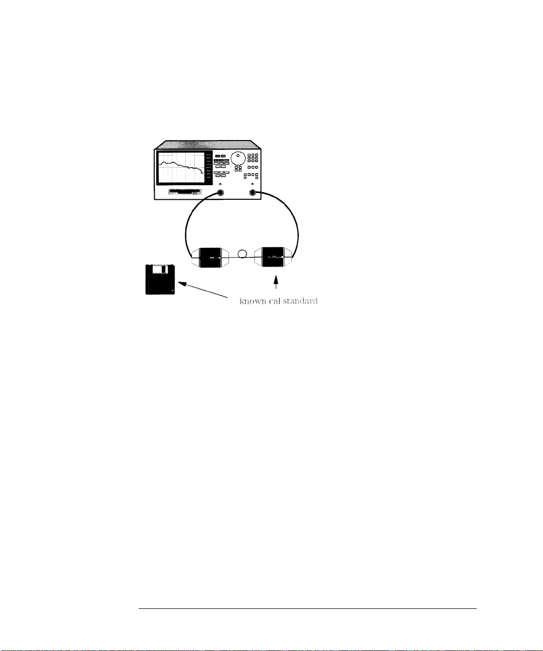
Measuring Lightwave Receivers

Measuring Phase Distortion

Connect the system as shown in Figure 3-4.

Figure 3-4. Phase Distortion CAL Test Setup

Select the measurement parameters and perform a response calibration.

PRESET, MEAS AVG

IF BW

POWER

LIGHTWAVE PARAMETERS

100, x1

, 10, x1,

RETURN

Trans: O/E (PORT 1→2)

STOP, 2, G/n

The IF bandwidth is decreased to reduce the effects of noise, the power is increased to +10 dBm to get better dynamic range, and the modulation stop frequency is set just about the device under test’s bandwidth.

Load the receiver CAL DATA from the disk into the analyzer by pressing:

CAL

CAL KITS & STDS, RECEIVER STANDARDS, LOAD RCVR DISC MENU

Be sure the file title matches the serial number of the receiver and then press the corresponding softkey,

LOAD RCVR1 DISK

LOAD RCVR2 DISK

, and wait until

the files have been loaded.

Perform the calibration be pressing:

DISK(2)

To save the data, press

Select the phase format to view the calibrated phase response of the receiver

3-12

SAVE/RECALL

CAL

CALIBRATE MENU, RESPONSE, DISK(1)

SAVE STATE

by pressing:

Measuring Lightwave Receivers

Measuring Phase Distortion

FORMAT

PHASE

The display should look similar to Figure 3-5, except for the markers. The markers on the example plot help to explain how phase is displayed on the analyzer. Note that the X-axis is the modulation frequency range and the Y-axis is phase, set to 90 degrees per division:

Marker 1 is at 0 degrees, marker 2 is at –180 degrees, marker 3 is near +180 degrees, and marker 4 is near 0 degrees (–3.1778 degrees). Better resolution can be obtained by increasing the number of points.

You can set the marker to any frequency and read the phase shift for that frequency on the display.

Figure 3-5. Calibrated Receiver System Phase Response

3-13

Measuring Lightwave Receivers

Measuring Phase Distortion

Insert the O/E device under test into the system in place of the receiver. Figure

3-6 shows the phase response of the diode receiver.

Figure 3-6. Phase Response of O/E (photo diode) Device Under Test

3-14

Measuring Lightwave Receivers

Measuring Phase Distortion

To measure the electrical delay or transmit time through the device under test, you must add enough electrical length or delay to the device to flatten out the phase response as close to zero degrees as possible. Adding electrical delay is a mathematical function that attempts to remove the length of the device by adding the delay to the measurement data. Press:

SCALE REF

ELECTRICAL DELAY

, then rotate (clockwise) the front panel knob until

the trace is as flat as possible, similar to Figure 3-7.

Figure 3-7. Electrical Delay Used to Flatten Phase Response

3-15

Measuring Lightwave Receivers

Measuring Phase Distortion

Obtain great resolution be pressing:

SCALE REF

SCALE/DIV

If necessary, readjust

, 10,

ELECTRICAL DELAY

so that the trace is as flat as possible across most of the band. Figure 3-8 shows an electrical transit time of 1.886 ns through the device under test. In this example, about 6 degrees of deviation from linear phase are shown across the band within the markers, approximately 1.56 MHz. To view the deviation at any particular modulation frequency, simply put the marker on that value and read the display.

Figure 3-8. Deviation from Linear Phase of O/E Device Under Test (Diode)

3-16

Measuring Electrical Devices

Always perform error corrections

Before making a measurement, you must correct the test setup for any systematic errors at the current measurement settings. Refer to “Procedures for Error-Correcting Measurements” on page 13-21 for the procedures. These procedures require that calibration kits, which mathematically describe test setup components, be saved in the HP 8702D’s internal memory. Most of these calibration kits have already been loaded at the factory. To learn about calibration kits, refer to Chapter 13, “Performing Calibrations”.

4-2

Measuring Electrical Devices

What you’ll find in this chapter

4-3

Measuring Electrical Devices

Measuring Magnitude and Insertion Phase Response

The HP 8702D allows you to make two different measurements simultaneously. You can make these measurements in different formats for the same parameter. For example, you could measure both the magnitude and phase of transmission. You could also measure two different parameters (S

To measure the magnitude and phase response

Connect your test device as shown in Figure 4-1.

and S22).

Figure 4-1. Device Connections for Measuring a Magnitude Response

4-4

Measuring Electrical Devices

Measuring Magnitude and Insertion Phase Response

Press

PRESET

and choose the measurement settings. For this example, the

measurement settings are as follows:

MEAS

Trans: E/E S21 FWD

CENTER, 134, M/ SPAN, 50, M/ MENU

POWER

SCALE REF

, –3,

AUTO SCALE

CHAN 2 MEAS

Trans: E/E S21 FWD

SCALE REF

AUTO SCALE

You may also want to select settings for the number of data points, averaging, and IF bandwidth.

Substitute a thru for the device and perform a frequency response measurement correction for both channel 1 and channel 2.

Reconnect your test device.

To better view the measurement trace, press:

CHAN 1, SCALE REF

To locate the maximum amplitude of the device response, as shown in Figure

AUTO SCALE

4-2, press:

MARKER FCTN

MKR SEARCH, SEARCH: MAX

4-5

Measuring Electrical Devices

Measuring Magnitude and Insertion Phase Response

Figure 4-2. Example Magnitude Response Measurement Results

To view both the magnitude and phase response of the device, as shown in

Figure 4-3, press:

CHAN 2 DISPLAY FORMAT

DUAL CHAN ON

PHASE

The channel 2 portion of Figure 4-3 shows the insertion phase response of the device under test. The analyzer measures and displays phase over the range of –180° to +180°. As phase changes beyond these values, a sharp 360° transition occurs in the displayed data.

The phase response shown in Figure 4-4 is undersampled; that is, there is more than 180° phase delay between frequency points. The frequency span should be reduced, or the number of points increased until ∆φ is less than 180° per point. Electrical delay may also be used to compensate for this effect.

4-6

Measuring Magnitude and Insertion Phase Response

Figure 4-3. Example Insertion Phase Response Measurement

Measuring Electrical Devices

4-7

Measuring Electrical Devices

Measuring Magnitude and Insertion Phase Response

∆φ

If the

= >180°, incorrect phase and delay information may result. The responses shown in Figure 4-3 have a ∆φ = >180° between two adjacent frequency points. Figure 4-4 shows an example of phase samples with ∆φ less than 180° and greater than 180°.

Figure 4-4. Maximum Amplitude of SAW Filter in Phase Format

4-8

Measuring Electrical Devices

Measuring Electrical Length and Phase Distortion

Measure changing phase by adding electrical delay

Electrical delay simulates a variable length lossless transmission line, which you can add to or remove from the HP 8702D’s receiver input to compensate for devices such as interconnecting cables.

Linearly changing phase is due to a device’s electrical length. You can measure this changing phase by adding electrical length (electrical delay) to compensate for it. A marker-to-delay function can be used to calculate the electrical delay by taking a ±10% span about the marker, measuring the ∆φ, and computing the delay as ∆φ/∆ frequency.

The measurement value that the HP 8702D displays represents the electrical length of your device relative to the speed of light in free space. The physical length of your device is related to this value by the propagation velocity of its medium. You could use the velocity factor to compensate for propagation velocity, helping the HP 8702D to measure correctly.

VELOCITY FACTOR

softkey function to change the

Phase distortion

The HP 8702D allows you to measure the linearity of the phase shift through a device over a range of frequencies and the HP 8702D can express it in two different ways: deviation from linear phase or group delay.

By adding electrical length to “flatten out” the phase response, you have removed the linear phase shift through your device. The deviation from linear phase shift through your device is all that remains. Refer to Figure 4-10.

4-9

Measuring Electrical Devices

Measuring Electrical Length and Phase Distortion

Group delay

The phase linearity of many devices is specified in terms of group or envelope delay. The HP 8702D can translate phase distortion into a related parameter, group delay. Group delay is the transmission time through your device as a function of frequency. Mathematically, it is the derivative of the phase response which can be approximated by the following ratio:

∆φ / (360 * ∆F)

where ∆φ is the difference in phase at two frequencies separated by ∆F.

The quantity ∆F is commonly called the “aperture” of the measurement. The HP 8702D calculates group delay from its phase response measurements. The default aperture is the total frequency span divided by the number of points across the display (in this example, 201 points or 0.5% of the total span).

4-10

Measuring Electrical Devices

Measuring Electrical Length and Phase Distortion

Group delay principles

For many networks, the amount of insertion phase is not as important as the linearity of the phase shift over a range of frequencies. The analyzer can measure this linearity and express it in two different ways: directly, as deviation from linear phase, or as group delay, a derived value.

Group delay is the measurement of signal transmission time through a test device. It is defined as the derivative of the phase characteristic with respect to frequency. Since the derivative is basically the instantaneous slope (or rate of change of phase with respect to frequency), a perfectly linear phase shift results in a constant slope, and therefore a constant group delay (refer to Fig-

ure 4-5).

Figure 4-5. Constant Group Delay

4-11

Measuring Electrical Devices

Measuring Electrical Length and Phase Distortion

Note, however, that the phase characteristic typically consists of both linear and higher order (deviations from linear) components. The linear component can be attributed to the electrical length of the test device, and represents the average signal transit time. The higher order components are interpreted as variations in transit time for different frequencies, and represent a source of signal distortion (refer to Figure 4-6).

Figure 4-6. Higher Order Phase Shift

4-12

Measuring Electrical Devices

Measuring Electrical Length and Phase Distortion

The analyzer computes group delay from the phase slope. Phase data is used to find the phase change, ∆φ, over a specified frequency aperture, ∆f, to obtain an approximation for the rate of change of phase with frequency (refer to Fig-

ure 4-7). This value,

, represents the group delay in seconds assuming linear

g phase change over ∆f. It is important that ∆φ be ≤180°, or errors will result in the group delay data. These errors can be significant for long delay devices. You can verify that ∆φ is ≤180° by increasing the number of points or narrowing the frequency span (or both) until the group delay data no longer changes.

Figure 4-7. Rate of Phase Change Versus Frequency

4-13

Measuring Electrical Devices

Measuring Electrical Length and Phase Distortion

When deviations from linear phase are present, changing the frequency step can result in different values for group delay. Note that in this case the computed slope varies as the aperture ∆f is increased (refer to Figure 4-8). A wider aperture results in loss of the fine grain variations in group delay. This loss of detail is the reason that, in any comparison of group delay data, it is important to know the aperture used to make the measurement.

Figure 4-8. Variations in Frequency Aperture

In determining the group delay aperture, there is a trade-off between resolution of fine detail and the effects of noise. Noise can be reduced by increasing the aperture, but this will tend to smooth out the fine detail. More detail will become visible as the aperture is decreased, but the noise will also increase, possibly to the point of obscuring the detail. A good practice is to use a smaller aperture to assure that small variations are not missed, then increase the aperture to smooth the trace.

The default group delay aperture is the frequency span divided by the number of points across the display. To set the aperture to a different value, turn on smoothing in the average menu, and vary the smoothing aperture. The aperture can be varied up to 20% of the span swept.

4-14

Measuring Electrical Devices

Measuring Electrical Length and Phase Distortion

Group delay measurements can be made on linear frequency, log frequency, or list frequency sweep types (not in CW or power sweep). Group delay aperture varies depending on the frequency spacing and point density, therefore the aperture is not constant in log and list frequency sweep modes. In list frequency mode, extra frequency points can be defined to ensure the desired aperture.

To obtain a readout of aperture values at different points on the trace, turn on

AVG

a marker. Then press

SMOOTHING APERTURE

. Smoothing aperture becomes the active function, and as the aperture is varied its value in Hz is displayed below the active entry area.

Electrical delay

ELECTRICAL DELAY

The

softkey, which is accessible from the

SCALE REF

key, adjusts the electrical delay to balance the phase of the test device. It simulates a variable length lossless transmission line, which can be added to or removed from a receiver input to compensate for interconnecting cables, etc. This function is similar to the mechanical or analog “line stretchers” of other analyzers. Delay is annotated in units of time with secondary labeling in distance for the current velocity factor.

With this feature, and with

MARKER →

DELAY

, an equivalent length of air-filled, lossless transmission line is added or subtracted according to the following formula:

Length (meters)= φ / (Freq in MHz × 1.20083)

Once the linear portion of the test device’s phase has been removed, the equivalent length of the lossless transmission line can be read out in the active marker area. If the average relative permittivity (

) of the test device is

r known over the frequency span, the length calculation can be adjusted to indicate the actual length of the test device more closely. This can be done by entering the relative velocity factor for the test device using the calibrate more menu. The relative velocity factor for a given dielectric can be calculated by:

Velocity Facto r= 1 ÷ square root of

(assuming a relative permeability of 1)

4-15

Measuring Electrical Devices

Measuring Electrical Length and Phase Distortion

To measure electrical length

Connect your test device as shown in Figure 4-9.

Figure 4-9. Device Connections for Measuring Electrical Length

PRESET

Press

MEAS

CENTER, 134, M/ SPAN, 2, M/ MENU

FORMAT SCALE REF

and choose the measurement settings. For example, press:

Trans: E/E S21 FWD

POWER

, 5, x1

PHASE

AUTO SCALE

Substitute a thru for the device and perform a frequency response measurement correction.

Reconnect your test device.

To better view the measurement trace, press

SCALE REF

AUTO SCALE

You may need to make the frequency span wider to see the effects of phase shift.

4-16

Figure 4-10. Linearly Changing Phase

Measuring Electrical Devices

Measuring Electrical Length and Phase Distortion

MARKER

Press

MARKER FCTN

and turn the front panel knob.

MARKER→DELAY

Turn the front panel knob to increase the electrical length until you achieve the best flat line, as shown in Figure 4-11.

If you know the velocity factor, press

CAL

MORE, VELOCITY FACTOR

and enter the

value, followed by x1.

Figure 4-11. Example Best Flat Line with Added Electrical Delay

To display the electrical length, press

SCALE REF

ELECTRICAL DELAY.

4-17

Measuring Electrical Devices

Measuring Electrical Length and Phase Distortion

To measure phase distortion

Follow the procedure in “To measure electrical length” on page 4-16.

Press

SCALE REF

SCALE DIV

and turn the front panel knob to increase the scale

resolution.

To use the marker statistics to measure the maximum peak-to-peak deviation from linear phase, press

Activate and adjust the electrical delay to obtain a minimum peak-to-peak

MARKER FCTN

MARKER MODE MENU, STATS ON

value.

It is possible to use delta markers to measure peak-to-peak deviation in only one portion of the trace, refer to “To calculate the statistics of the measurement data” on page 7-29.

Figure 4-12. Deviation From Linear Phase Example Measurement

4-18

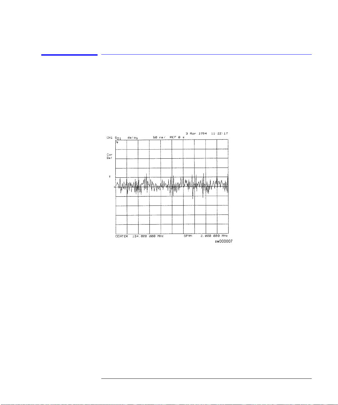
Measuring Electrical Devices

Measuring Electrical Length and Phase Distortion

To measure group delay

Perform the procedure “To measure phase distortion” on page 4-18.

FORMAT

Press

To activate a marker to measure the group delay at a particular frequency,

MARKER

press

and turn the front panel knob.

DELAY,

SCALE REF

SCALE DIV,

↑, ↑.

Figure 4-13. Group Delay Example Measurement

To vary the effective group delay aperture from minimum aperture (no

AVG

smoothing) to approximately 1% of the frequency span, press

SMOOTHING

Group delay measurements may require a specific aperture (∆f) or frequency spacing between measurement points. The phase shift between two adjacent frequency points must be less than 180°, otherwise incorrect group delay information may result. When you increase the aperture, the HP 8702D removes fine grain variations from the response. It is critical that you specify the group delay aperture when you compare group delay measurements.

4-19

Measuring Electrical Devices

Measuring Electrical Length and Phase Distortion

Figure 4-14. Group Delay Example Measurement with Smoothing

To increase the effective group delay aperture, by increasing the number of measurement points over which the HP 8702D calculates the group delay,

SMOOTHING APERTURE

press

, 5, x1.

As the aperture is increased the “smoothness” of the trace improves markedly, but at the expense of measurement detail.

4-20

Agilent 8702D Users Guide

Specifications and Main Features

Frequently Asked Questions

User Manual

Contents

A Quick Tour

Front panel

Display

Rear panel

Changing Instrument Settings

Making Measurements Using Guided Setup

To make an O/E measurement

Setting the RF Output

Defining the frequency range

Understanding the power ranges

Power coupling options

Source attenuator switch protection

Sweep time

Sweep types

Alternate and chop sweep modes

Protecting Against Electrostatic Damage

Cleaning Connections for Accurate Measurements

Cleaning Optical Connectors

To clean a non-lensed connector

To clean an adapter

To test insertion loss and return loss

Cleaning Electrical Connections

Making Transmission Measurements

To measure a source

Making Reflection Measurements

Making Transmission Measurements

To measure a receiver

Making Reflection Measurements

Measuring Phase Distortion

Measuring Magnitude and Insertion Phase Response

To measure the magnitude and phase response

Measuring Electrical Length and Phase Distortion

Group delay principles

Electrical delay

To measure electrical length

To measure phase distortion

To measure group delay