Agilent 86100A Programmer’s Guide

DCA and DCA-J

Agilent 86100A/B/C Wide-Bandwidth Oscilloscope Programmer’s Guide

Notices

No part of this manual may be reproduced in any form or by any means (including electronic storage and retrieval or translation into a foreign language) without prior agreement and written consent from Agilent Technologies, Inc. as governed by United States and international copyright lays.

Manual Part Number

86100-90065

Edition

First edition, February 2004

Printed in Malaysia

Agilent Technologies, Inc. Digital Signal Analysis Division 1400 Fountaingrove Parkway Santa Rosa, CA 95403, USA

Warranty

The material contained in this document is provided “as is,” and is subject to being changed, without notice, in future editions. Further, to the maximum extent permitted by applicable law, Agilent disclaims all warranties, either express or implied, with regard to this manual and any information contained herein, including but not limited to the implied warranties of merchantability and fitness for a particular purpose. Agilent shall not be liable for errors or for incidental or consequential damages in connection with the furnishing, use, or performance of this document or of any information contained herein. Should Agilent and the user have a separate written agreement with warranty terms covering the material in this document that conflict with these terms, the warranty terms in the separate agreement shall control.

Technology Licenses

The hardware and/or software described in this document are furnished under a license and may be used or copied only in accordance with the terms of such license.

Departments and Agencies of the U.S. Government will receive no greater than Restricted Rights as defined in FAR

52.227-19(c)(1-2) (June 1987). U.S. Government users will receive no greater than Limited Rights as defined in FAR

52.227-14 (June 1987) or DFAR 252.2277015 (b)(2) (November 1995), as applicable in any technical data.

Safety Notices

CAUTION

Caution denotes a hazard. It calls attention to a procedure which, if not correctly performed or adhered to, could result in damage to or destruction of the product. Do not proceed beyond a caution sign until the indicated conditions are fully understood and met.

WARNING

Warning denotes a hazard. It calls attention to a procedure which, if not correctly performed or adhered to, could result in injury or loss of life. Do not proceed beyond a warning sign until the indicated conditions are fully understood and met.

LZW compression/decompression: Licensed under U.S. Patent No. 4,558,302 and foreign counterparts. The purchase or use of LZW graphics capability in a licensed product does not authorize or permit an end user to use any other product or perform any other method or activity involving use of LZW unless the end user is separately licensed in writing by Unisys.

Restricted Rights Legend

If software is for use in the performance of a U.S. Government prime contract or subcontract, Software is delivered and licensed as “Commercial computer software” as defined in DFAR 252.227-7014 (June 1995), or as a “commercial item” as defined in FAR 2.101(a) or as “Restricted computer software” as defined in FAR

52.227-19 (June 1987) or any equivalent agency regulation or contract clause. Use, duplication or disclosure of Software is subject to Agilent Technologies’ standard commercial license terms, and non-DOD

Contents

1Introduction

Getting Started Programming 1-12 Interface Functions 1-17 Status Reporting 1-20 Message Communication and System Functions 1-34 Programming Conventions 1-37 Multiple Databases 1-47 Language Compatibility 1-50 New and Revised Commands 1-56 Commands Unavailable in Jitter Mode 1-58 Error Messages 1-60

2Sample Programs

Sample Program Structure 2-3 Sample C Programs 2-4 Listings of the Sample Programs 2-20

3 Common Commands

4 Root Level Commands

5 System Commands

6 Acquire Commands

7 Calibration Commands

8 Channel Commands

9 Clock Recovery Commands

10 Disk Commands

11 Display Commands

12 Function Commands

Contents-1

Contents

13 Hardcopy Commands

14 Histogram Commands

15 Limit Test Commands

16 Marker Commands

17 Mask Test Commands

18 Measure Commands

19 TDR/TDT Commands

20 Timebase Commands

21 Trigger Commands

22 Waveform Commands

23 Waveform Memory Commands

Contents-2

Introduction

This chapter introduces the basics for remote programming of an analyzer. The programming commands in this manual conform to the IEEE 488.2 Standard Digital Interface for Programmable Instrumentation. The programming commands provide the means of remote control.

Basic operations that you can do with a computer (GPIB controller) and an analyzer include:

• Set up the analyzer.

• Make measurements.

• Get data (waveform, measurements, configuration) from the analyzer.

• Send information, such as waveforms and configurations, to the analyzer.

Communicating with the Analyzer

Other tasks are accomplished by combining these functions.

Example Programs are Written in HP BASIC and C

The programming examples for individual commands in this manual are written in HP BASIC and C.

Computers communicate with the analyzer by sending and receiving messages over a remote interface, usually with GPIB programming. Commands for programming normally appear as ASCII character strings embedded in the output statements of a “host” language available on your computer. The input commands of the host language are used to read in responses from the analyzer.

For example, HP BASIC uses the OUTPUT statement for sending commands and queries. After a query is sent, the response is usually read using the HP BASIC ENTER statement. The ENTER statement passes the value across the bus to the computer and places it in the designated variable.

For the GPIB interface, messages are placed on the bus using an output command and passing the device address, program message, and a terminator. Passing the device address ensures that the program message is sent to the correct GPIB interface and GPIB device.

This HP BASIC OUTPUT statement sends a command that sets the channel 1 scale value to 500 mV:

1-2

Introduction

OUTPUT <device address>;":CHANNEL1:SCALE 500E-3"<terminator>

The device address represents the address of the device being programmed. Each of the other parts of the above statement are explained in the following pages.

Use the Suffix Multiplier Instead

Using "mV" or "V" following the numeric voltage value in some commands will cause Error 138–Suffix not allowed. Instead, use the convention for the suffix multiplier as described in “Message Communication and System Functions” on page 1-34.

Output Command The output command depends entirely on the programming language. Throughout this

book, HP BASIC and ANSI C are used in the examples of individual commands. If you are using other languages, you will need to find the equivalents of HP BASIC commands like OUTPUT, ENTER, and CLEAR, to convert the examples.

Device Address The location where the device address must be specified depends on the programming

language you are using. In some languages, it may be specified outside the OUTPUT command. In HP BASIC, it is always specified after the keyword OUTPUT. The examples in this manual assume that the analyzer and interface card are at GPIB device address 707. When writing programs, the device address varies according to how the bus is configured.

Instructions Instructions, both commands and queries, normally appear as strings embedded in a

statement of your host language, such as HP BASIC, Pascal, or C. The only time a parameter is not meant to be expressed as a string is when the instruction's syntax definition specifies <block data>, such as HP BASIC’s "learnstring" command. There are only a few instructions that use block data.

Instructions are composed of two main parts:

• The header, which specifies the command or query to be sent.

• The program data, which provides additional information to clarify the meaning of the instruction.

Instruction Header

The instruction header is one or more command mnemonics separated by colons (:) that represent the operation to be performed by the analyzer. See “Programming Conventions” on page 1-37 for more information.

Queries are formed by adding a question mark (?) to the end of the header. Many instructions can be used as either commands or queries, depending on whether or not you include the question mark. The command and query forms of an instruction usually have different program data. Many queries do not use any program data.

1-3

Introduction

White Space (Separator)

White space is used to separate the instruction header from the program data. If the instruction does not require any program data parameters, you do not need to include any white space. In this manual, white space is defined as one or more spaces. ASCII defines a space to be character 32, in decimal.

Program Data Program data is used to clarify the meaning of the command or query. It provides nec-

essary information, such as whether a function should be on or off or which waveform is to be displayed. Each instruction's syntax definition shows the program data, and the values they accept. See “Numeric Program Data” on page 1-7 for more information about general syntax rules and acceptable values.

When there is more than one data parameter, they are separated by commas (,). You can add spaces around the commas to improve readability.

Header Types There are three types of headers:

• Simple Command headers

• Compound Command headers

• Common Command headers

Simple Command Header

Simple command headers contain a single mnemonic. AUTOSCALE and DIGITIZE are examples of simple command headers typically used in this analyzer. The syntax is:

OUTPUT 707;”:AUTOSCALE”

When program data must be included with the simple command header (for example, :DIGITIZE CHAN1), white space is added to separate the data from the header. The syntax is:

OUTPUT 707;”:DIGITIZE CHANNEL1,FUNCTION2”

Compound Command Header

Compound command headers are a combination of two program mnemonics. The first mnemonic selects the subsystem, and the second mnemonic selects the function within that subsystem. The mnemonics within the compound message are separated by colons. For example:

To execute a single function within a subsystem:

:<subsystem>:<function><separator><program data><terminator>

For example:

1-4

Introduction

OUTPUT 707;”:CHANNEL1:BANDWIDTH HIGH”

Combining Commands in the Same Subsystem

To execute more than one command within the same subsystem, use a semi-colon (;) to separate the commands:

:<subsystem>:<command><separator><data>;<command><separator><data><terminator>

For example:

:CHANNEL1:DISPLAY ON;BWLIMIT ON

Common Command Header

Common command headers, such as clear status, control the IEEE 488.2 functions within the analyzer. The syntax is:

*<command header><terminator>

No space or separator is allowed between the asterisk (*) and the command header. *CLS is an example of a common command header.

Duplicate Mnemonics

Identical function mnemonics can be used for more than one subsystem. For example, the function mnemonic RANGE may be used to change the vertical range or to change the horizontal range.

To set the vertical range of channel 1 to 0.4 volts full scale:

:CHANNEL1:RANGE .4

To set the horizontal time base to 1 second full scale:

:TIMEBASE:RANGE 1

CHANNEL1 and TIMEBASE are subsystem selectors, and determine which range is being modified.

Query Headers Command headers immediately followed by a question mark (?) are queries. After

receiving a query, the analyzer interrogates the requested subsystem and places the answer in its output queue. The answer remains in the output queue until it is read or until another command is issued. When read, the answer is transmitted across the bus to the designated listener (typically a computer). For example, the query:

:TIMEBASE:RANGE?

places the current time base setting in the output queue.

In HP BASIC, the computer input statement:

ENTER < device address >;Range

1-5

Introduction

passes the value across the bus to the computer and places it in the variable Range.

You can use query commands to find out how the analyzer is currently configured. They are also used to get results of measurements made by the analyzer. For example, the command:

:MEASURE:RISETIME?

tells the analyzer to measure the rise time of your waveform and place the result in the output queue.

The output queue must be read before the next program message is sent. For example, when you send the query :MEASURE:RISETIME? you must follow it with an input statement. In HP BASIC, this is usually done with an ENTER statement immediately followed by a variable name. This statement reads the result of the query and places the result in a specified variable.

Handling Queries Properly

If you send another command or query before reading the result of a query, the output buffer is cleared and the current response is lost. This also generates a query-interrupted error in the error queue. If you execute an input statement before you send a query, it will cause the computer to wait indefinitely.

Program Header Options

You can send program headers using any combination of uppercase or lowercase ASCII characters. Analyzer responses, however, are always returned in uppercase.

You may send program command and query headers in either long form (complete spelling), short form (abbreviated spelling), or any combination of long form and short form. For example:

:TIMEBASE:DELAY 1E-6 is the long form. :TIM:DEL 1E-6 is the short form.

Using Long Form or Short Form

Programs written in long form are easily read and are almost self-documenting. The short form syntax conserves the amount of computer memory needed for program storage and reduces I/O activity.

The rules for the short form syntax are described in “Programming Conventions” on page 1-37.

1-6

Introduction

Character Program Data

Numeric Program Data

Character program data is used to convey parameter information as alpha or alphanumeric strings. For example, the :TIMEBASE:REFERENCE command can be set to left, center, or right. The character program data in this case may be LEFT, CENTER, or RIGHT. The command :TIMEBASE:REFERENCE RIGHT sets the time base reference to right.

The available mnemonics for character program data are always included with the instruction's syntax definition. Either the long form of commands, or the short form (if one exists), may be sent. Uppercase and lowercase letters may be mixed freely. When receiving responses, uppercase letters are used exclusively.

Some command headers require program data to be expressed numerically. For example, :TIMEBASE:RANGE requires the desired full scale range to be expressed numerically.

For numeric program data, you can use exponential notation or suffix multipliers to indicate the numeric value. The following numbers are all equal:

28 = 0.28E2 = 280E-1 = 28000m = 0.028K = 28E-3K

When a syntax definition specifies that a number is an integer, it means that the number should be whole. Any fractional part is ignored and truncated. Numeric data parameters that accept fractional values are called real numbers. For more information see “Interface Functions” on page 1-17.

All numbers are expected to be strings of ASCII characters.

• When sending the number 9, you would send a byte representing the ASCII code for the character “9” (which is 57).

Embedded Strings

Program Message Terminator

• A three-digit number like 102 would take up three bytes (ASCII codes 49, 48, and 50). The number of bytes is figured automatically when you include the entire instruction in a string.

Embedded strings contain groups of alphanumeric characters which are treated as a unit of data by the analyzer. An example of this is the line of text written to the advisory line of the analyzer with the :SYSTEM:DSP command:

:SYSTEM:DSP ""This is a message.""

You may delimit embedded strings with either single (') or double (") quotation marks. These strings are case-sensitive, and spaces act as legal characters just like any other character.

The program instructions within a data message are executed after the program message terminator is received. The terminator may be either a NL (New Line) character, an EOI (End-Or-Identify) asserted in the GPIB interface, or a combination of the two. Asserting the EOI sets the EOI control line low on the last byte of the data message. The NL character is an ASCII linefeed (decimal 10).

1-7

Introduction

New Line Terminator Functions Like EOS and EOT

The NL (New Line) terminator has the same function as an EOS (End Of String) and EOT (End Of Text) terminator.

Common Commands within a Subsystem

Selecting Multiple Subsystems

Common commands can be received and processed by the analyzer whether they are sent over the bus as separate program messages or within other program messages. If you have selected a subsystem, and a common command is received by the analyzer, the analyzer remains in the selected subsystem. For example, if the program message

":ACQUIRE:AVERAGE ON;*CLS;COUNT 1024"

is received by the analyzer, the analyzer turns averaging on, then clears the status information without leaving the selected subsystem.

If some other type of command is received within a program message, you must reenter the original subsystem after the command. For example, the program message

":ACQUIRE:AVERAGE ON;:AUTOSCALE;:ACQUIRE:AVERAGE:COUNT 1024"

turns averaging on, completes the autoscale operation, then sets the acquire average count. In this example, :ACQUIRE must be sent again after the AUTOSCALE command to re-enter the ACQUIRE subsystem and set count.

You can send multiple program commands and program queries for different subsystems on the same line by separating each command with a semicolon. The colon following the semicolon lets you enter a new subsystem. For example:

:CHANNEL1:RANGE 0.4;:TIMEBASE:RANGE 1

You Can Combine Compound and Simple Commands

Multiple commands may be any combination of compound and simple commands.

File Names and Types

When specifying a file name in a remote command, enclose the name in double quotation marks, such as "filename". If you specify a path, the path should be included in the quotation marks.

You can use the full path name, a relative path name, or no path. For example, you can specify:

• a full path name: "D:\User Files\waveforms\channel2.wfm"

• a relative path name: "..\myfile.set" or “.\screen1.jpg”

• a simple file name: "Memory1.txt"

1-8

Introduction

All files stored using remote commands have file name extensions.The following table shows the file name extension used for each file type.

Table 1-1. File Name Extensions

File Type File Name Extension

Waveform - internal format .wfm

Waveform - text format (Verbose or Y values) .txt

Setup .set

Color grade - Gray Scale .cgs

Jitter Memory .jd

Screen image .bmp, .eps, .gif, .pcx, .ps, .jpg, .tif

Mask .msk, .pcm

TDR/TDT .tdr

If you do not specify an extension when storing a file, or specify an incorrect extension, it will be corrected automatically according to the following rules:

• No extension specified: add the extension for the file type.

• Extension does not match file type: retain the filename, (including the current extension) and add the appropriate extension.

You do not need to use an extension when loading a file if you use the optional destination parameter. For example, :DISK:LOAD "STM1_OC3",SMASK will automatically add .msk to the file name.

Note

For .gif and .tif file formats, this instrument uses LZW compression/decompression licensed under U.S. patent No 4,558,302 and foreign counterparts. End user should not modify, copy, or distribute LZW compression/decompression capability.

For .jpg file format, this instrument uses the .jpg software written by the Independent JPEG Group.

1-9

Introduction

The following table shows the rules used when loading a specified file.

Table 1-2. Rules for Loading Files

File Name Extension Destination Rule

No extension Not specified Default to internal waveform format; add .wfm

extension

Extension does not match file type

Extension matches file type Not specified Use file name with no alterations; destination is

No extension Specified Add extension for destination type; default for

Extension does not match destination file type

Extension matches destination file type

Not specified Default to internal waveform format; add .wfm

extension

based on extension file type

waveforms is internal format (.wfm)

Specified Retain file name; add extension for destination

type. Default for waveforms is internal format (.wfm)

Specified Retain file name; destination is as specified

Note

ASCII waveform files can be loaded only if the file name explicitly includes the .txt extension.

File Locations If you don’t specify a directory when storing a file, the location of the file will be based

on the file type. The following table shows the default locations for storing files. On 86100C instruments, files are stored on the D: drive. On 86100A/B instruments, files are stored on the C: drive.

Table 1-3. Default File Locations for Storing Files (1 of 2)

File Type Default Location

Waveform - internal format D:\User Files\waveforms

Waveform - text format (Verbose or Y values) D:\User Files\waveforms

Setup D:\User Files\setups

Color Grade - Gray Scale D:\User Files\colorgrade-grayscale

Jitter Memory D:\User Files\jitter data

Screen Image D:\User Files\screen images

Mask C:\Scope\masks (standard masks)

D:\User Files\masks (user-defined masks)

1-10

Introduction

Table 1-3. Default File Locations for Storing Files (2 of 2)

File Type Default Location

TDR/TDT calibration data D:\User Files\TDR normalization

When loading a file, you can specify the full path name, a relative path name, or no path name. The following table shows the rules for locating files, based on the path specified.

Table 1-4. File Locations (Loading Files)

File Name Rule

Full path name Use file name and path specified

Relative path name Full path name is formed relative to the present

working directory, set with the command :DISK:CDIR. The present working directory can be read with the query :DISK:PWD?

File name with no preceding path Add the file name to the default path

(D:\User Files) based on the file type.

Standard masks loaded from C:\Scope\masks. Files may be stored to or loaded from any path external drive or on any mapped network drive.

1-11

Introduction

Getting Started Programming

The remainder of this chapter discusses how to set up the analyzer, how to retrieve setup information and measurement results, how to digitize a waveform, and how to pass data to the computer. Chapter 18, “Measure Commands” describes sending measurement data to the analyzer.

Initialization To make sure the bus and all appropriate interfaces are in a known state, begin every

program with an initialization statement. For example, HP BASIC provides a CLEAR command which clears the interface buffer:

CLEAR 707 ! initializes the interface of the analyzer

When you are using GPIB, CLEAR also resets the analyzer's parser. The parser is the program that reads in the instructions you send.

After clearing the interface, initialize the analyzer to a preset state:

OUTPUT 707;"*RST" ! initializes the analyzer to a preset state

Initializing the analyzer

The commands and syntax for initializing the analyzer are discussed in Chapter 3, “Common Commands”. Refer to your GPIB manual and programming language reference manual for information on initializing the interface.

Autoscale

The AUTOSCALE feature of Agilent Technologies digitizing analyzers performs a very useful function on unknown waveforms by automatically setting up the vertical channel, time base, and trigger level of the analyzer.

The syntax for the autoscale function is:

:AUTOSCALE<terminator>

Setting Up the Analyzer

A typical analyzer setup configures the vertical range and offset voltage, the horizontal range, delay time, delay reference, trigger mode, trigger level, and slope.

A typical example of the commands sent to the analyzer are:

:CHANNEL1:RANGE 16;OFFSET 1.00<terminator> :SYSTEM:HEADER OFF<terminator> :TIMEBASE:RANGE 1E-3;DELAY 100E-6<terminator>

1-12

Introduction

Getting Started Programming

This example sets the time base at 1 ms full-scale (100 µs/div), with delay of 100 µs. Vertical is set to 16 V full-scale (2 V/div), with center of screen at 1 V, and probe attenuation of 10.

Example Program This program demonstrates the basic command structure used to program the ana-

lyzer.

10 CLEAR 707 ! Initialize analyzer interface 20 OUTPUT 707;"*RST" !Initialize analyzer to preset state 30 OUTPUT 707;":TIMEBASE:RANGE 5E-4"! Time base to 500 us full scale 40 OUTPUT 707;":TIMEBASE:DELAY 25E-9"! Delay to 25 ns 50 OUTPUT 707;":TIMEBASE:REFERENCE CENTER"! Display reference at center 60 OUTPUT 707;":CHANNEL1:RANGE .16"! Vertical range to 160 mV full scale 70 OUTPUT 707;":CHANNEL1:OFFSET -.04"! Offset to -40 mV 80 OUTPUT 707;":TRIGGER:LEVEL,-.4"! Trigger level to -0.4 90 OUTPUT 707;":TRIGGER:SLOPE POSITIVE"! Trigger on positive slope 100 OUTPUT 707;":SYSTEM:HEADER OFF"<terminator> 110 OUTPUT 707;":DISPLAY:GRATICULE FRAME"! Grid off 120 END

Overview of the Program

• Line 10 initializes the analyzer interface to a known state.

• Line 20 initializes the analyzer to a preset state.

Using the DIGITIZE Command

• Lines 30 through 50 set the time base, the horizontal time at 500

µs full scale,

and 25 ns of delay referenced at the center of the graticule.

• Lines 60 through 70 set the vertical range to 160 millivolts full scale and the center screen at

• Lines 80 through 90 configure the analyzer to trigger at

−40 millivolts.

−0.4 volts with normal

triggering.

• Line 100 turns system headers off.

• Line 110 turns the grid off.

The DIGITIZE command is a macro that captures data using the acquisition (ACQUIRE) subsystem. When the digitize process is complete, the acquisition is stopped. The captured data can then be measured by the analyzer or transferred to the computer for further analysis. The captured data consists of two parts: the preamble and the waveform data record.

After changing the analyzer configuration, the waveform buffers are cleared. Before doing a measurement, the DIGITIZE command should be sent to ensure new data has been collected.

You can send the DIGITIZE command with no parameters for a higher throughput. Refer to the DIGITIZE command in Chapter 4, “Root Level Commands” for details.

1-13

Introduction

Getting Started Programming

When the DIGITIZE command is sent to an analyzer, the specified channel’s waveform is digitized with the current ACQUIRE parameters. Before sending the :WAVEFORM:DATA? query to get waveform data, specify the WAVEFORM parameters.

The number of data points comprising a waveform varies according to the number requested in the ACQUIRE subsystem. The ACQUIRE subsystem determines the number of data points, type of acquisition, and number of averages used by the DIGITIZE command. This allows you to specify exactly what the digitized information contains. The following program example shows a typical setup:

OUTPUT 707;":SYSTEM:HEADER OFF"<terminator> OUTPUT 707;":WAVEFORM:SOURCE CHANNEL1"<terminator> OUTPUT 707;":WAVEFORM:FORMAT BYTE"<terminator> OUTPUT 707;":ACQUIRE:COUNT 8"<terminator> OUTPUT 707;":ACQUIRE:POINTS 500"<terminator> OUTPUT 707;":DIGITIZE CHANNEL1"<terminator> OUTPUT 707;":WAVEFORM:DATA?"<terminator>

This setup places the analyzer to acquire eight averages. This means that when the DIGITIZE command is received, the command will execute until the waveform has been averaged at least eight times.

After receiving the :WAVEFORM:DATA? query, the analyzer will start passing the waveform information when queried.

Digitized waveforms are passed from the analyzer to the computer by sending a numerical representation of each digitized point. The format of the numerical representation is controlled with the :WAVEFORM:FORMAT command and may be selected as BYTE, WORD, or ASCII.

The easiest method of entering a digitized waveform depends on data structures, available formatting, and I/O capabilities. You must scale the integers to determine the voltage value of each point. These integers are passed starting with the leftmost point on the analyzer's display. For more information, refer to Chapter 22, “Waveform Commands”.

When using GPIB, a digitize operation may be aborted by sending a Device Clear over the bus (for example, CLEAR 707).

Receiving Information from the Analyzer

Note

The execution of the DIGITIZE command is subordinate to the status of ongoing limit tests. (See commands ACQuire:RUNTil on page 6-5, MTEST:RUNTil on page 17-10, and LTEST:RUNTil on page 15-5.) The DIGITIZE command will not capture data if the stop condition for a limit test has been met.

After receiving a query (command header followed by a question mark), the analyzer places the answer in its output queue. The answer remains in the output queue until it is read or until another command is issued. When read, the answer is transmitted across the interface to the computer. The input statement for receiving a response

1-14

Introduction

Getting Started Programming

message from an analyzer's output queue typically has two parameters; the device address and a format specification for handling the response message. For example, to read the result of the query command :CHANNEL1:RANGE? you would execute the HP BASIC statement:

ENTER <device address>;Setting$

The device address parameter represents the address of the analyzer. This would enter the current setting for the range in the string variable Setting$.

All results for queries sent in a program message must be read before another program message is sent. For example, when you send the query :MEASURE:RISETIME?, you must follow that query with an input statement. In HP BASIC, this is usually done with an ENTER statement.

Handling Queries Properly

If you send another command or query before reading the result of a query, the output buffer will be cleared and the current response will be lost. This will also generate a query-interrupted error in the error queue. If you execute an input statement before you send a query, it will cause the computer to wait indefinitely.

The format specification for handling response messages depends on both the computer and the programming language.

String Variable Example

Numeric Variable Example

The output of the analyzer may be numeric or character data, depending on what is queried. Refer to the specific commands for the formats and types of data returned from queries.

For the example programs, assume that the device being programmed is at device address 707. The actual address depends on how you have configured the bus for your own application.

In HP BASIC 5.0, string variables are case-sensitive, and must be expressed exactly the same way each time they are used. This example shows the data being returned to a string variable:

10 DIM Rang$[30] 20 OUTPUT 707;":CHANNEL1:RANGE?" 30 ENTER 707;Rang$ 40 PRINT Rang$ 50 END

After running this program, the computer displays:

+8.00000E-01

This example shows the data being returned to a numeric variable:

10 OUTPUT 707;":CHANNEL1:RANGE?" 20 ENTER 707;Rang

1-15

Introduction

Getting Started Programming

30 PRINT Rang 40 END

After running this program, the computer displays:

Definite-Length Block Response Data

Definite-length block response data allows any type of device-dependent data to be transmitted over the system interface as a series of 8-bit binary data bytes. This is particularly useful for sending large quantities of data or 8-bit extended ASCII codes. The syntax is a pound sign (#) followed by a non-zero digit representing the number of digits in the decimal integer. After the non-zero digit is the decimal integer that states the number of 8-bit data bytes being sent. This is followed by the actual data.

For example, for transmitting 4000 bytes of data, the syntax would be:

#44000 <4000 bytes of data> <terminator>

The leftmost “4” represents the number of digits in the number of bytes, and “4000” represents the number of bytes to be transmitted.

Multiple Queries You can send multiple queries to the analyzer within a single program message, but you

must also read them back within a single program message. This can be accomplished by either reading them back into a string variable or into multiple numeric variables. For example, you could read the result of the query :TIMEBASE:RANGE?;DELAY? into the string variable Results$ with the command:

ENTER 707;Results$

When you read the result of multiple queries into string variables, each response is separated by a semicolon. For example, the response of the query :TIMEBASE:RANGE?;DELAY? would be:

<range_value>;<delay_value>

Use the following program message to read the query :TIMEBASE:RANGE?;DELAY? into multiple numeric variables:

ENTER 707;Result1,Result2

Analyzer Status Status registers track the current status of the analyzer. By checking the analyzer sta-

tus, you can find out whether an operation has completed, is receiving triggers, and more. “Status Reporting” on page 1-20 explains how to check the status of the analyzer.

1-16

Introduction

Interface Functions

The interface functions deal with general bus management issues, as well as messages that can be sent over the bus as bus commands. In general, these functions are defined by IEEE 488.1.

GPIB Interface Connector

The analyzer is equipped with a GPIB interface connector on the rear panel. This allows direct connection to a GPIB equipped computer. You can connect an external GPIB compatible device to the analyzer by installing a GPIB cable between the two units. Finger tighten the captive screws on both ends of the GPIB cable to avoid accidentally disconnecting the cable during operation.

A maximum of fifteen GPIB compatible instruments (including a computer) can be interconnected in a system by stacking connectors. This allows the analyzers to be connected in virtually any configuration, as long as there is a path from the computer to every device operating on the bus.

CAUTION Avoid stacking more than three or four cables on any one connector. Multiple

connectors produce leverage that can damage a connector mounting.

GPIB Default Startup Conditions

The following default GPIB conditions are established during power-up: 1) The Request Service (RQS) bit in the status byte register is set to zero. 2) All of the event registers, the Standard Event Status Enable Register, Service Request Enable Register, and the Status Byte Register are cleared.

1-17

Introduction

Interface Functions

Interface Capabilities

The interface capabilities of this analyzer, as defined by IEEE 488.1, are listed in the following table.

Table 1-5. Interface Capabilities

Code Interface Function Capability

SH1 Source Handshake Full Capability

AH1 Acceptor Handshake Full Capability

T5 Talker Basic Talker/Serial Poll/Talk Only Mode/

Unaddress if Listen Address (MLA)

L4 Listener Basic Listener/

Unaddresses if Talk Address (MTA)

SR1 Service Request Full Capability

RL1 Remote Local Complete Capability

PP1 Parallel Poll Remote Configuration

DC1 Device Clear Full Capability

DT1 Device Trigger Full Capability

C0 Computer No Capability

E2 Driver Electronics Tri State (1 MB/SEC MAX)

Command and Data Concepts

Communicating Over the Bus

The GPIB has two modes of operation, command mode and data mode. The bus is in the command mode when the Attention (ATN) control line is true. The command mode is used to send talk and listen addresses and various bus commands such as group execute trigger (GET).

The bus is in the data mode when the ATN line is false. The data mode is used to convey device-dependent messages across the bus. The device-dependent messages include all of the analyzer specific commands, queries, and responses found in this manual, including analyzer status information.

Device addresses are sent by the computer in the command mode to specify who talks and who listens. Because GPIB can address multiple devices through the same interface card, the device address passed with the program message must include the correct interface select code and the correct analyzer address.

Device Address = (Interface Select Code * 100) + (Analyzer Address)

1-18

Introduction

Interface Functions

The Analyzer is at Address 707 in Examples

The examples in this manual assume that the analyzer is at device address 707.

Interface Select Code

Each interface card has a unique interface select code. This code is used by the computer to direct commands and communications to the proper interface. The default is typically “7” for GPIB interface cards.

Analyzer Address

Each analyzer on the GPIB must have a unique analyzer address between decimal 0 and 30. This analyzer address is used by the computer to direct commands and communications to the proper analyzer on an interface. The default is typically “7” for this analyzer. You can change the analyzer address in the Utilities, Remote Interface dialog box.

Do Not Use Address 21 for an Analyzer Address

Address 21 is usually reserved for the Computer interface Talk/Listen address and should not be used as an analyzer address.

Bus Commands

The following commands are IEEE 488.1 bus commands (ATN true). IEEE 488.2 defines many of the actions that are taken when these commands are received by the analyzer.

Device Clear

The device clear (DCL) and selected device clear (SDC) commands clear the input buffer and output queue, reset the parser, and clear any pending commands. If either of these commands is sent during a digitize operation, the digitize operation is aborted.

Group Execute Trigger

The group execute trigger (GET) command arms the trigger. This is the same action produced by sending the RUN command.

Interface Clear

The interface clear (IFC) command halts all bus activity. This includes unaddressing all listeners and the talker, disabling serial poll on all devices, and returning control to the system computer.

1-19

Introduction

Status Reporting

An overview of the analyzer's status reporting structure is shown in the following figure. The status reporting structure shows you how to monitor specific events in the analyzer. Monitoring these events allows determination of the status of an operation, the availability and reliability of the measured data, and more.

• To monitor an event, first clear the event, then enable the event. All of the events are cleared when you initialize the analyzer.

• To generate a service request (SRQ) interrupt to an external computer, enable at least one bit in the Status Byte Register.

The Status Byte Register, the Standard Event Status Register group, and the Output Queue are defined as the Standard Status Data Structure Model in IEEE 488.2-1987. IEEE 488.2 defines data structures, commands, and common bit definitions for status reporting. There are also analyzer-defined structures and bits.

Status Reporting Data Structures

The different status reporting data structures, descriptions, and interactions are shown in the following figure. To make it possible for any of the Standard Event Status Register bits to generate a summary bit, the corresponding bits must be enabled. These bits are enabled by using the *ESE common command to set the corresponding bit in the Standard Event Status Enable Register.

To generate a service request (SRQ) interrupt to the computer, at least one bit in the Status Byte Register must be enabled. These bits are enabled by using the *SRE common command to set the corresponding bit in the Service Request Enable Register. These enabled bits can then set RQS and MSS (bit 6) in the Status Byte Register.

For more information about common commands, see Chapter 3, “Common Commands”.

1-20

Introduction

Status Reporting

Figure 1-1. Status Reporting Overview Block Diagram

The status reporting structure consists of the registers shown in this figure.

The following table lists the bit definitions for each bit in the status reporting data structure.

Table 1-6. Status Reporting Bit Definition (1 of 3)

Bit Description Definition

PON Power On Indicates power is turned on.

1-21

Introduction

Status Reporting

Table 1-6. Status Reporting Bit Definition (Continued) (2 of 3)

Bit Description Definition

URQ Not used. Permanently set to zero.

CME Command Error Indicates if the parser detected an error.

EXE Execution Error Indicates if a parameter was out of range or was

inconsistent with the current settings.

DDE Device Dependent Error Indicates if the device was unable to complete an

operation for device dependent reasons.

QYE Query Error Indicates if the protocol for queries has been violated.

RQL Request Control Indicates if the device is requesting control.

OPC Operation Complete Indicates if the device has completed all pending

operations.

OPER Operation Status

RQS Request Service Indicates that the device is requesting service.

MSS Master Summary Status Indicates if a device has a reason for requesting service.

ESB Event Status Bit Indicates if any of the enabled conditions in the Standard

MAV Message Available Indicates if there is a response in the output queue.

MSG Message Indicates if an advisory has been displayed.

USR User Event Register Indicates if any of the enabled conditions have occurred

TRG Trigger Indicates if a trigger has been received.

LCL Local Indicates if a remote-to-local transition occurs.

FAIL Fail Indicates the specified test has failed.

COMP Complete Indicates the specified test has completed.

LTEST Limit Test Indicates that one of the enabled conditions in the Limit

MTEST Mask Test Indicates that one of the enabled conditions in the Mask

Indicates if any of the enabled conditions in the Operation Status Register have occurred.

Event Status Register have occurred.

in the User Event Register.

Test Register has occurred.

1-22

Introduction

Status Reporting

Table 1-6. Status Reporting Bit Definition (Continued) (3 of 3)

Bit Description Definition

ACQ Acquisition Indicates that acquisition test has completed in the

Acquisition Register.

CLCK CloCk Indicates that one of the enabled conditions in the Clock

Recovery Register has occurred.

UNLK UNLoCKed Indicates that an unlocked or trigger loss condition has

occurred in the Clock Recovery Module.

LOCK LOCKed Indicates that a locked or trigger capture condition has

occurred in the Clock Recovery Module.

NSPR1 No Signal Present

Receiver 1

SPR1 Signal Present

Receiver 1

NSPR2 No Signal Present

Receiver 2

SPR2 Signal Present

Receiver 2

LOSS Time Reference Loss Indicates the Precision Timebase (provided by the

PTIME Precision Timebase Indicates that one of the enabled conditions in the

Indicates that the Clock Recovery Module has detected the loss of an optical signal on receiver one.

Indicates that the Clock Recovery Module has detected an optical signal on receiver one.

Indicates that the Clock Recovery Module has detected the loss of an optical signal on receiver two.

Indicates that the Clock Recovery Module has detected an optical signal on receiver two.

Agilent 86107A module) has detected a time reference loss due to a change in the reference clock signal.

Precision Timebase Register has occurred.

1-23

Introduction

Status Reporting

Figure 1-2. Status Reporting Data Structures

1-24

Introduction

Status Reporting

Status Reporting Data Structures (continued)

1-25

Introduction

Status Reporting

Status Byte Register

The Status Byte Register is the summary-level register in the status reporting structure. It contains summary bits that monitor activity in the other status registers and queues. The Status Byte Register is a live register. That is, its summary bits are set and cleared by the presence and absence of a summary bit from other event registers or queues.

If the Status Byte Register is to be used with the Service Request Enable Register to set bit 6 (RQS/MSS) and to generate an SRQ, at least one of the summary bits must be enabled, then set. Also, event bits in all other status registers must be specifically enabled to generate the summary bit that sets the associated summary bit in the Status Byte Register.

The Status Byte Register can be read using either the *STB? common command query or the GPIB serial poll command. Both commands return the decimal-weighted sum of all set bits in the register. The difference between the two methods is that the serial poll command reads bit 6 as the Request Service (RQS) bit and clears the bit which clears the SRQ interrupt. The *STB? query reads bit 6 as the Master Summary Status (MSS) and does not clear the bit or have any affect on the SRQ interrupt. The value returned is the total bit weights of all of the bits that are set at the present time.

The use of bit 6 can be confusing. This bit was defined to cover all possible computer interfaces, including a computer that could not do a serial poll. The important point to remember is that, if you are using an SRQ interrupt to an external computer, the serial poll command clears bit 6. Clearing bit 6 allows the analyzer to generate another SRQ interrupt when another enabled event occurs.

The only other bit in the Status Byte Register affected by the *STB? query is the Message Available bit (bit 4). If there are no other messages in the Output Queue, bit 4 (MAV) can be cleared as a result of reading the response to the *STB? query.

If bit 4 (weight = 16) and bit 5 (weight = 32) are set, a program would print the sum of the two weights. Since these bits were not enabled to generate an SRQ, bit 6 (weight =

64) is not set.

Example 1

This HP BASIC example uses the *STB? query to read the contents of the analyzer’s Status Byte Register when none of the register's summary bits are enabled to generate an SRQ interrupt.

10 OUTPUT 707;":SYSTEM:HEADER OFF;*STB?"!Turn headers off 20 ENTER 707;Result!Place result in a numeric variable 30 PRINT Result!Print the result 40 End

The next program prints 132 and clears bit 6 (RQS) of the Status Byte Register. The difference in the decimal value between this example and the previous one is the value of bit 6 (weight = 64). Bit 6 is set when the first enabled summary bit is set, and is cleared when the Status Byte Register is read by the serial poll command.

1-26

Introduction

Status Reporting

Example 2

This example uses the HP BASIC serial poll (SPOLL) command to read the contents of the analyzer’s Status Byte Register.

10 Result = SPOLL(707) 20 PRINT Result 30 END

Use Serial Polling to Read the Status Byte Register

Serial polling is the preferred method to read the contents of the Status Byte Register because it resets bit 6 and allows the next enabled event that occurs to generate a new SRQ interrupt.

Service Request Enable Register

Trigger Event Register (TRG)

Setting the Service Request Enable Register bits enables corresponding bits in the Status Byte Register. These enabled bits can then set RQS and MSS (bit 6) in the Status Byte Register.

Bits are set in the Service Request Enable Register using the *SRE command, and the bits that are set are read with the *SRE? query. Bit 6 always returns 0. Refer to the Status Reporting Data Structures shown in Figure 1-2.

Example

This example sets bit 4 (MAV) and bit 5 (ESB) in the Service Request Enable Register.

OUTPUT 707;"*SRE 48"

This example uses the parameter “48” to allow the analyzer to generate an SRQ interrupt under the following conditions:

• When one or more bytes in the Output Queue set bit 4 (MAV).

• When an enabled event in the Standard Event Status Register generates a summary bit that sets bit 5 (ESB).

This register sets the TRG bit in the status byte when a trigger event occurs.

The TRG event register stays set until it is cleared by reading the register or using the *CLS (clear status) command. If your application needs to detect multiple triggers, the TRG event register must be cleared after each one.

If you are using the Service Request to interrupt a computer operation when the trigger bit is set, you must clear the event register after each time it is set.

1-27

Introduction

Status Reporting

Standard Event Status Register

The Standard Event Status Register (SESR) monitors the following analyzer status events:

• PON - Power On

• CME - Command Error

• EXE - Execution Error

• DDE - Device Dependent Error

• QYE - Query Error

• RQC - Request Control

• OPC - Operation Complete

When one of these events occurs, the corresponding bit is set in the register. If the corresponding bit is also enabled in the Standard Event Status Enable Register, a summary bit (ESB) in the Status Byte Register is set.

The contents of the Standard Event Status Register can be read and the register cleared by sending the *ESR? query. The value returned is the total bit weights of all of the bits set at the present time.

Example

This example uses the *ESR? query to read the contents of the Standard Event Status Register.

10 OUTPUT 707;":SYSTEM:HEADER OFF"!Turn headers off 20 OUTPUT 707;"*ESR?" 30 ENTER 707;Result!Place result in a numeric variable 40 PRINT Result!Print the result 50 End

Standard Event Status Enable Register

If bit 4 (weight = 16) and bit 5 (weight = 32) are set, the program prints the sum of the two weights.

For any of the Standard Event Status Register (SESR) bits to generate a summary bit, you must first enable the bit. Use the *ESE (Event Status Enable) common command to set the corresponding bit in the Standard Event Status Enable Register. Set bits are read with the *ESE? query.

Example

Suppose your application requires an interrupt whenever any type of error occurs. The error status bits in the Standard Event Status Register are bits 2 through 5. The sum of the decimal weights of these bits is 60. Therefore, you can enable any of these bits to generate the summary bit by sending:

OUTPUT 707;"*ESE 60"

Whenever an error occurs, the analyzer sets one of these bits in the Standard Event Status Register. Because the bits are all enabled, a summary bit is generated to set bit 5 (ESB) in the Status Byte Register.

1-28

Introduction

Status Reporting

If bit 5 (ESB) in the Status Byte Register is enabled (via the *SRE command), a service request interrupt (SRQ) is sent to the external computer.

Disabled SESR Bits Respond, but Do Not Generate a Summary Bit

Standard Event Status Register bits that are not enabled still respond to their corresponding conditions (that is, they are set if the corresponding event occurs). However, because they are not enabled, they do not generate a summary bit in the Status Byte Register.

User Event Register (UER)

Local Event Register (LCL)

Operation Status Register (OPR)

This register hosts the LCL bit (bit 0) from the Local Events Register. The other 15 bits are reserved. You can read and clear this register using the UER? query. This register is enabled with the UEE command. For example, if you want to enable the LCL bit, you send a mask value of 1 with the UEE command; otherwise, send a mask value of 0.

This register sets the LCL bit in the User Event Register and the USR bit (bit 1) in the Status byte. It indicates a remote-to-local transition has occurred. The LER? query is used to read and to clear this register.

This register hosts the CLCK bit (bit 7), the LTEST bit (bit 8), the ACQ bit (bit 9) and the MTEST bit (bit 10).

The CLCK bit is set when any of the enabled conditions in the Clock Recovery Event Register have occurred.

The LTEST bit is set when a limit test fails or is completed and sets the corresponding FAIL or COMP bit in the Limit Test Events Register.

The ACQ bit is set when the COMP bit is set in the Acquisition Event Register, indicating that the data acquisition has satisfied the specified completion criteria.

The MTEST bit is set when the Mask Test either fails specified conditions or satisfies its completion criteria, setting the corresponding FAIl or COMP bits in the Mask Test Events Register.

The PTIME bit is set when there is a loss of the precision timebase reference occurs setting a bit in the Precision Timebase Events Register.

The JIT bit is set in Jitter Mode when a bit is set in the Jitter Events Register. This occurs when there is a failure or an autoscale is needed.

If any of these bits are set, the OPER bit (bit 7) of the Status Byte register is set. The Operation Status Register is read and cleared with the OPER? query. The register output is enabled or disabled using the mask value supplied with the OPEE command.

Clock Recovery Event Register (CRER)

This register hosts the UNLK bit (bit 0), LOCK bit (bit 1), NSPR1 bit (bit 2), SPR1 bit (bit 3), NSPR2 bit (bit 4) and SPR2 (bit 5).

Bit 0 (UNLK) of the Clock Recovery Event Register is set when an 83491/2/3/4/5A Clock Recovery module becomes unlocked or trigger loss has occurred.

1-29

Introduction

Status Reporting

Bit 1 (LOCK) of the Clock Recovery Event Register is set when an 83491/2/3/4/5A Clock Recovery module becomes locked or a trigger capture has occurred.

Bit 2 (NSPR1) of the Clock Recovery Event Register is set when an 83491/2/3/4A Clock Recovery module transitions to no longer detecting an optical signal on receiver one. An 83495A module does not affect this bit.

Bit 3 (SPR1) of the Clock Recovery Event Register is set when an 83491/2/3/4A Clock Recovery module transitions to detecting an optical signal on receiver one. An 83495A module does not affect this bit.

Bit 4 (NSPR2) of the Clock Recovery Event Register is set when an 83491/2/3/4A Clock Recovery module transitions to no longer detecting an optical signal on receiver two. An 83495A module does not affect this bit.

Bit 5 (SPR2) of the Clock Recovery Event Register is set when an 83491/2/3/4A Clock Recovery module transitions to detecting an optical signal on receiver two. An 83495A module does not affect this bit.

The Clock Recovery Event Register is read and cleared with the CRER? query.

When either of the UNLK, LOCK, NSPR1, SPR1, NSPR2 or SPR2 bits are set, they in turn set CLCK bit (bit 7) of the Operation Status Register. Results from the Clock Recovery Event Register can be masked by using the CREE command to set the Clock Recovery Event Enable Register. Refer to the CREE command in Chapter 4, “Root Level Commands” for enable and mask value definitions.

Limit Test Event Register (LTER)

Acquisition Event Register (AER)

Bit 0 (COMP) of the Limit Test Event Register is set when the Limit Test completes. The Limit Test completion criteria are set by the LTESt:RUN command.

Bit 1 (FAIL) of the Limit Test Event Register is set when the Limit Test fails. Failure criteria for the Limit Test are defined by the LTESt:FAIL command.

The Limit Test Event Register is read and cleared with the LTER? query.

When either the COMP or FAIL bits are set, they in turn set the LTEST bit (bit 8) of the Operation Status Register. You can mask the COMP and FAIL bits, thus preventing them from setting the LTEST bit, by defining a mask using the LTEE command.

Enable Mask Value

Block COMP and FAIL 0 Enable COMP, block FAIL 1 Enable FAIL, block COMP 2 Enable COMP and FAIL 3

Bit 0 (COMP) of the Acquisition Event Register is set when the acquisition limits complete. The Acquisition completion criteria are set by the ACQuire:RUNtil command. The Acquisition Event Register is read and cleared with the ALER? query.

1-30

Introduction

Status Reporting

When the COMP bit is set, it in turn sets the ACQ bit (bit 9) of the Operation Status Register. Results from the Acquisition Register can be masked by using the AEEN command to set the Acquisition Event Enable Register to the value 0. You enable the COMP bit by setting the mask value to 1.

Mask Test Event Register (MTER)

Precision Timebase Event Register (PTER)

Bit 0 (COMP) of the Mask Test Event Register is set when the Mask Test completes. The Mask Test completion criteria are set by the MTESt:RUMode command.

Bit 1 (FAIL) of the Mask Test Event Register is set when the Mask Test fails. This will occur whenever any sample is recorded within any region defined in the mask.

The Mask Test Event Register is read and cleared with the MTER? query.

When either the COMP or FAIL bits are set, they in turn set the MTEST bit (bit 10) of the Operation Status Register. You can mask the COMP and FAIL bits, thus preventing them from setting the MTEST bit, by setting corresponding bits to zero using the MTEE command.

Enable Mask Value

Block COMP and FAIL 0 Enable COMP, block FAIL 1 Enable FAIL, block COMP 2 Enable COMP and FAIL 3

Bit 0 (LOSS) of the Precision Timebase Event Register is set when loss of the time reference occurs. Time reference is lost when a change in the amplitude or frequency of the reference clock signal is detected. The Precision Timebase Event Register is read and cleared with the PTER? query.

When the LOSS bit is set, it in turn sets the PTIME bit (bit 11) of the Operation Status Register. Results from the Precision Timebase Register can be masked by using the PTEE command to set the Precision Timebase Event Enable Register to the value 0. You enable the LOSS bit by setting the mask value to 1.

Jitter Event Register (JIT)

Install the Precision Timebase Module

The Precision Timebase feature requires the installation of the Agilent 86107A Precision Timebase Module.

Bit 0 of the Jitter Event Register is set when characterizing edges in Jitter Mode fails. Bit 1 of the register is set when pattern synchronization is lost in Jitter Mode. Bit 2 of the register is set when a parameter change in Jitter Mode has made autoscale necessary. Bit 12 of the Operation Status Register (JIT) indicates that one of the enabled conditions in the Jitter Event Register has occurred.

1-31

Introduction

Status Reporting

Error Queue As errors are detected, they are placed in an error queue. This queue is first in, first

out. If the error queue overflows, the last error in the queue is replaced with error –350, “Queue overflow”. Any time the queue overflows, the oldest errors remain in the queue, and the most recent error is discarded. The length of the analyzer's error queue is 30 (29 positions for the error messages, and 1 position for the “Queue overflow” message).

The error queue is read with the SYSTEM:ERROR? query. Executing this query reads and removes the oldest error from the head of the queue, which opens a position at the tail of the queue for a new error. When all the errors have been read from the queue, subsequent error queries return 0, “No error.”

The error queue is cleared when any of the following occurs:

• When the analyzer is powered up.

• When the analyzer receives the *CLS common command.

• When the last item is read from the error queue.

For more information on reading the error queue, refer to the SYSTEM:ERROR? query in Chapter 5, “System Commands”. For a complete list of error messages, refer to “Error Messages” on page 1-60.

Output Queue The output queue stores the analyzer-to-computer responses that are generated by

certain analyzer commands and queries. The output queue generates the Message Available summary bit when the output queue contains one or more bytes. This summary bit sets the MAV bit (bit 4) in the Status Byte Register. The output queue may be read with the HP BASIC ENTER statement.

Message Queue The message queue contains the text of the last message written to the advisory line on

the screen of the analyzer. The queue is read with the SYSTEM:DSP? query. Note that messages sent with the SYSTem:DSP command do not set the MSG status bit in the Status Byte Register.

Clearing Registers and Queues

The *CLS common command clears all event registers and all queues except the output queue. If *CLS is sent immediately following a program message terminator, the output queue is also cleared.

1-32

Introduction

Status Reporting

Figure 1-3. Status Reporting Decision Chart

1-33

Introduction

Message Communication and System Functions

This chapter describes the operation of analyzers that operate in compliance with the IEEE 488.2 (syntax) standard. It is intended to give you enough basic information about the IEEE 488.2 standard to successfully program the analyzer. You can find additional detailed information about the IEEE 488.2 standard in ANSI/IEEE Std 488.21987, “IEEE Standard Codes, Formats, Protocols, and Common Commands.”

This analyzer series is designed to be compatible with other Agilent Technologies IEEE

488.2 compatible instruments. Analyzers that are compatible with IEEE 488.2 must also be compatible with IEEE 488.1 (GPIB bus standard); however, IEEE 488.1 compatible analyzers may or may not conform to the IEEE 488.2 standard. The IEEE 488.2 standard defines the message exchange protocols by which the analyzer and the computer will communicate. It also defines some common capabilities that are found in all IEEE 488.2 analyzers.

This chapter also contains some information about the message communication and system functions not specifically defined by IEEE 488.2.

Protocols

The message exchange protocols of IEEE 488.2 define the overall scheme used by the computer and the analyzer to communicate. This includes defining when it is appropriate for devices to talk or listen, and what happens when the protocol is not followed.

Functional Elements

Input Buffer The input buffer of the analyzer is the memory area where commands and queries are

Output Queue The output queue of the analyzer is the memory area where all output data, or

Before proceeding with the description of the protocol, you should understand a few system components.

stored prior to being parsed and executed. It allows a computer to send a string of commands, which could take some time to execute, to the analyzer, then proceed to talk to another analyzer while the first analyzer is parsing and executing commands.

response messages, are stored until read by the computer.

1-34

Introduction

Message Communication and System Functions

Parser The analyzer's parser is the component that interprets the commands sent to the ana-

lyzer and decides what actions should be taken. “Parsing” refers to the action taken by the parser to achieve this goal. Parsing and execution of commands begins when either the analyzer recognizes a program message terminator, or the input buffer becomes full. If you want to send a long sequence of commands to be executed, then talk to another analyzer while they are executing, you should send all of the commands before sending the program message terminator.

Protocol Overview The analyzer and computer communicate using program messages and response mes-

sages. These messages serve as the containers into which sets of program commands or analyzer responses are placed.

A program message is sent by the computer to the analyzer, and a response message is sent from the analyzer to the computer in response to a query message. A query message is defined as being a program message that contains one or more queries. The analyzer will only talk when it has received a valid query message and, therefore, has something to say. The computer should only attempt to read a response after sending a complete query message, but before sending another program message.

Remember This Rule of Analyzer Communication

The basic rule to remember is that the analyzer will only talk when prompted to, and it then expects to talk before being told to do something else.

Protocol Operation

Protocol Exceptions

When the analyzer is turned on, the input buffer and output queue are cleared, and the parser is reset to the root level of the command tree.

The analyzer and the computer communicate by exchanging complete program messages and response messages. This means that the computer should always terminate a program message before attempting to read a response. The analyzer will terminate response messages except during a hardcopy output.

After a query message is sent, the next message should be the response message. The computer should always read the complete response message associated with a query message before sending another program message to the same analyzer.

The analyzer allows the computer to send multiple queries in one query message. This is referred to as sending a “compound query”. Multiple queries in a query message are separated by semicolons. The responses to each of the queries in a compound query will also be separated by semicolons.

Commands are executed in the order they are received.

If an error occurs during the information exchange, the exchange may not be completed in a normal manner.

1-35

Introduction

Message Communication and System Functions

Suffix Multiplier The suffix multipliers that the analyzer will accept are shown in Table 1-7.

Table 1-7. <suffix mult>

Value Mnemonic Value Mnemonic

1E18 EX 1E-3 m

1E15 PE 1E-6 u

1E12 T 1E-9 n

1E9 G 1E-12 p

1E6 MA 1E-15 f

1E3 K 1E-18 a

Suffix Unit The suffix units that the analyzer will accept are shown in Table 1-8.

Table 1-8. <suffix unit>

Suffix Referenced Unit

VVolt

s Second

WWatt

BIT Bits

dB Decibel

% Percent

Hz Hertz

1-36

Introduction

Programming Conventions

This chapter describes conventions used to program the Agilent 86100A, and conventions used throughout this manual. A block diagram and description of data flow is included for understanding analyzer operations. A description of the command tree and command tree traversal is also included. See the Quick Reference for more information about command syntax.

Data Flow The data flow gives you an idea of where the measurements are made on the acquired

data and when the post-signal processing is applied to the data.

The following figure is a block diagram of the analyzer. The diagram is laid out serially for a visual perception of how the data is affected by the analyzer.

Figure 1-4. Sample Data Processing

The sample data is stored in the channel memory for further processing before being displayed. The time it takes for the sample data to be displayed depends on the number of post processes you have selected.

Averaging your sampled data helps remove any unwanted noise from your waveform.

1-37

Introduction

Programming Conventions

You can store your sample data in the analyzer’s waveform memories for use as one of the sources in Math functions, or to visually compare against a waveform that is captured at a future time. The Math functions allow you to apply mathematical operations on your sampled data. You can use these functions to duplicate many of the mathematical operations that your circuit may be performing to verify that your circuit is operating correctly.

The measurements section performs any of the automated measurements that are available in the analyzer. The measurements that you have selected appear at the bottom of the display.

The Connect Dots section draws a straight line between sample data points, giving an analog look to the waveform. This is sometimes called linear interpolation.

Truncation Rule The following truncation rule is used to produce the short form (abbreviated spelling)

for the mnemonics used in the programming headers and alpha arguments.

Command Truncation Rule

The mnemonic is the first four characters of the keyword, unless the fourth character is a vowel. Then the mnemonic is the first three characters of the keyword. If the length of the keyword is four characters or less, this rule does not apply, and the short form is the same as the long form.

The Command Tree

The following table shows how the truncation rule is applied to commands.

Table 1-9. Mnemonic Truncation

Long Form Short Form How the Rule is Applied

RANGE RANG Short form is the first four characters of the keyword.

PATTERN PATT Short form is the first four characters of the keyword.

DISK DISK Short form is the same as the long form.

DELAY DEL Fourth character is a vowel, short form is the first three characters.

The command tree in Figure 1-5 on page 1-40 shows all of the commands in the Agilent 86100A and the relationship of the commands to each other. The IEEE 488.2 common commands are not listed as part of the command tree because they do not affect the position of the parser within the tree.

When a program message terminator (<NL>, linefeed - ASCII decimal 10) or a leading colon (:) is sent to the analyzer, the parser is set to the “root” of the command tree.

1-38

Introduction

Programming Conventions

Command Types

The commands in this analyzer can be placed into three types: common commands, root level commands, and subsystem commands.

• Common commands are commands defined by IEEE 488.2 and control some functions that are common to all IEEE 488.2 instruments. These commands are independent of the tree and do not affect the position of the parser within the tree. *RST is an example of a common command.

• Root level commands control many of the basic functions of the analyzer. These commands reside at the root of the command tree. They can always be parsed if they occur at the beginning of a program message or are preceded by a colon. Unlike common commands, root level commands place the parser back at the root of the command tree. AUTOSCALE is an example of a root level command.

• Subsystem commands are grouped together under a common node of the command tree, such as the TIMEBASE commands. Only one subsystem may be selected at a given time. When the analyzer is initially turned on, the command parser is set to the root of the command tree and no subsystem is selected.

Tree Traversal Rules

Command headers are created by traversing down the command tree. A legal command header from the command tree would be :TIMEBASE:RANGE. This is referred to as a compound header. A compound header is a header made up of two or more mnemonics separated by colons. The compound header contains no spaces. The following rules apply to traversing the tree.

Tree Traversal Rules

A leading colon or a program message terminator (<NL> or EOI true on the last byte) places the parser at the root of the command tree. A leading colon is a colon that is the first character of a program header. Executing a subsystem command places you in that subsystem until a leading colon or a program message terminator is found.

In the command tree, use the last mnemonic in the compound header as a reference point (for example, RANGE). Then find the last colon above that mnemonic (TIMEBASE:). That is the point where the parser resides. Any command below this point can be sent within the current program message without sending the mnemonics which appear above them (for example, REFERENCE).

1-39

Introduction

Programming Conventions

Figure 1-5. Command Tree

1-40

Introduction

Programming Conventions

Command Tree (Continued)

1-41

Introduction

Programming Conventions

Command Tree (Continued)

1-42

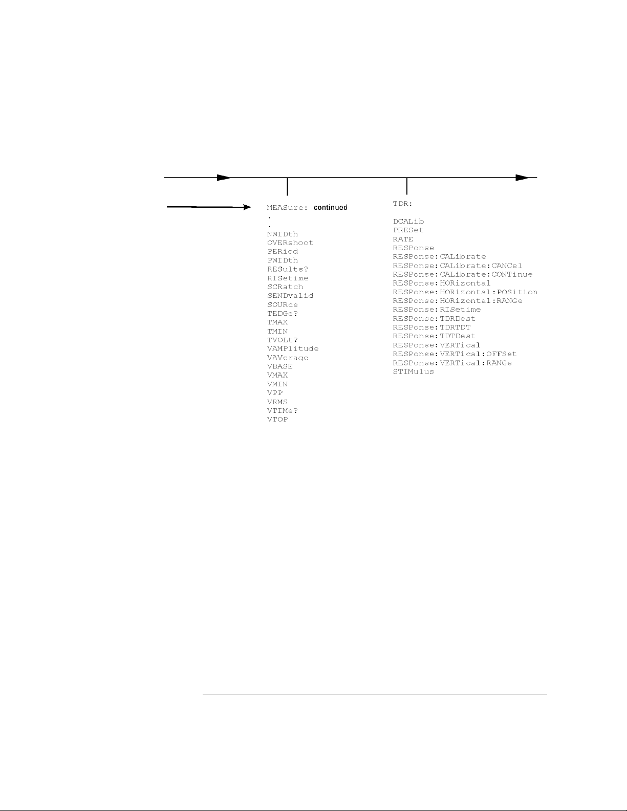
Introduction

Programming Conventions

Command Tree (Continued)

1-43

Introduction

Programming Conventions

Command Tree (Continued)

1-44

Introduction

Programming Conventions

Tree Traversal Examples

The OUTPUT statements in the following examples are written using HP BASIC 5.0. The quoted string is placed on the bus, followed by a carriage return and linefeed (CRLF).

Example 1

Consider the following command:

OUTPUT 707;":CHANNEL1:RANGE 0.5;OFFSET 0"

The colon between CHANNEL1 and RANGE is necessary because CHANNEL1:RANGE is a compound command. The semicolon between the RANGE command and the OFFSET command is required to separate the two commands or operations. The OFFSET command does not need CHANNEL1 preceding it because the CHANNEL1:RANGE command sets the parser to the CHANNEL1 node in the tree.

Example 2

Consider the following commands:

OUTPUT 707;":TIMEBASE:REFERENCE CENTER;POSITION 0.00001"

OUTPUT 707;":TIMEBASE:REFERENCE CENTER" OUTPUT 707;":TIMEBASE:POSITION 0.00001"

Infinity Representation

Sequential and Overlapped Commands

In the first line of example 2, the “subsystem selector” is implied for the POSITION command in the compound command.

A second way to send these commands is shown in the second part of the example. Since the program message terminator places the parser back at the root of the command tree, TIMEBASE must be reselected to re-enter the TIMEBASE node before sending the POSITION command.

Example 3

Consider the following command:

OUTPUT 707;":TIMEBASE:REFERENCE CENTER;:CHANNEL1:OFFSET 0"

In example 3, the leading colon before CHANNEL1 tells the parser to go back to the root of the command tree. The parser can then recognize the CHANNEL1:OFFSET command and enter the correct node.

The representation for infinity for this analyzer is 9.99999E+37. This is also the value returned when a measurement cannot be made.

IEEE 488.2 makes a distinction between sequential and overlapped commands.

Sequential commands finish their task before the execution of the next command starts.

1-45

Introduction

Programming Conventions

Overlapped commands run concurrently. Commands following an overlapped command may be started before the overlapped command is completed. The common commands *WAI and *OPC may be used to ensure that commands are completely processed before subsequent commands are executed.

Response

As defined by IEEE 488.2, query responses may be buffered for the following reasons:

Generation

• When the query is parsed by the analyzer.

• When the computer addresses the analyzer to talk so that it may read the response.

This analyzer buffers responses to a query when the query is parsed.

EOI The EOI bus control line follows the IEEE 488.2 standard without exception.

1-46

Introduction

Multiple Databases

Eye/Mask measurements in the Agilent 86100A are based on statistical data that is acquired and stored in the color grade/gray scale database. The color grade/gray scale database consists of all data samples displayed on the display graticule. The measurement algorithms are dependent upon histograms derived from the database. This database is internal to the instrument’s applications. The color grade/gray scale database cannot be imported into an external database application.

Eye/Mask Measurements

If you want to perform an eye measurement, it is necessary that you first produce an eye diagram by triggering the instrument with a synchronous clock signal. Measurements made on a pulse waveform while in Eye/Mask mode will fail.

Using Multiple Databases in Remote Programs

Firmware revision A.03.00 and later allows for multiple color grade/gray scale databases to be acquired and displayed simultaneously. This includes

• all four instrument channels

• all four math functions

• one saved color grade/gray scale file

The ability to use multiple databases allows for the comparison of

• channels to each other

• channels to a saved color grade/gray scale file

• functions to the channel data on which it is based

The advantage of acquiring and displaying channels and functions simultaneously is test times are greatly reduced. For example, the time taken to acquire two channels in parallel is approximately the same time taken to acquire a single channel.

You will notice that throughout this manual, most commands that control histograms, mask tests, or color grade data have additional optional parameters that were not available in firmware revisions prior to A.03.00. You can use the commands to control a single channel or add the argument APPend to enable more than one channel. The following example illustrates two uses of the CHANnel<n>:DISPlay command.

1-47

Introduction

Multiple Databases

SYSTem:MODE EYE CHANnel1:DISPlay ON CHANnel2:DISPlay ON

The result using the above set of commands, is Channel 1 cleared and disabled while Channel 2 is enabled and displayed.

However, by adding the argument APPend to the last command of the set, both Channels 1 and 2 will be enabled and displayed .

SYSTem:MODE EYE CHANnel1:DISPlay ON CHANnel2:DISPlay ON,APPend

For a example of using multiple databases, refer to “multidatabase.c Sample Program” on page 2-43.

Downloading a Database

The general process for downloading a color grade/gray scale database is as follows:

1 Send the command :WAVEFORM:SOURCE CGRADE

This will select the color grade/gray scale database as the waveform source.

2 Issue :WAVeform:FORMat WORD.

Database downloads only support word formatted data (16-bit integers).

3 Send the query :WAVeform:DATA?

The data will be sent by means of a block data transfer as a two-dimensional array, 450 words wide by 320 words high (refer to “Definite-Length Block Response Data” on page 1-16). The data is transferred starting with the upper left pixel of the display graticule, column by column, until the lower right pixel is transferred.

4 Send the command :WAVeform:XORigin to obtain the time of the left column.

5 Send the command :WAVeform:XINC to obtain the time increment of each

column.

6 Send the command :WAVeform:YORigin to obtain the voltage or power of the

vertical center of the database.

7 Send the command :WAVeform:YORigin to obtain the voltage or power of the

incremental row.

The information from steps 4 through 7 can also be obtained with the command :WAVeform:PREamble.

Auto Skew Another multiple database feature is the auto skew . You can use the auto skew feature

to lset the horizontal skew of multiple, active channels with the same bit rate, so that the waveform crossings align with each other. This can be very convient when viewing multiple eye diagrams simultaneously. Slight differences between channels and test

1-48

Introduction

Multiple Databases

devices may cause a phase difference between channels. Auto skew ensures that each eye is properly aligned, so that measurements and mask tests can be properly executed.

In addition, auto skew optimizes the instrument trigger level. Prior to auto skew, at least one channel must display a complete eye diagram in order to make the initial bit rate measurement.

Acquisition Time

Auto skew requires more data to be sampled; therefore, acquisition time during auto skew is slightly longer than acquisition time during measurements.

1-49

Introduction

Language Compatibility

This section lists Agilent 83480A commands that are not used in the Agilent 86100A

Agilent 83480A/54750A Programming Commands and Queries Not Used in the 86100A (1 of 6)

Programming Commands/Queries Replacement Commands/Queries

Common Commands

*LRN SYSTEM:SETUP

Root Level Commands

:AER? No replacement

:ERASe No replacement

:HEEN :AEEN

:MENU No replacement

:MERGe No replacement

:STORe:PMEMory1 No replacement

:TEER No replacement

System Commands :SYSTem

:SYSTem:KEY No replacement

Calibration Commands :CALibrate

:CALibrate:FRAMe:CANCel :CALibrate:CANcel

:CALibrate:FRAMe:CONTinue :CALibrate:CONTinue

:CALibrate:FRAMe:DATA No replacement

:CALibrate:FRAMe:DONE? :CALibrate:STATus?

:CALibrate:FRAMe:MEMory? No replacement

:CALibrate:PLUGin:ACCuracy :CALibrate:MODule:STATus

:CALibrate:PLUGin:CANCel :CALibrate:CANcel

:CALibrate:PLUGin:CONTinue :CALibrate:CONTinue

:CALibrate:PLUGin:DONE? :CALibrate:STATus?

1-50

Introduction

Language Compatibility

Agilent 83480A/54750A Programming Commands and Queries Not Used in the 86100A (2 of 6)

:CALibrate:PLUGin:MEMory? No replacement

:CALibrate:PLUGin:OFFSet :CALibrate:MODule:OFFSet

:CALibrate:PLUGin:OPOWer :CALibrate:MODule:OPOWer

:CALibrate:PLUGin:OPTical :CALibrate:MODule:OPTical

:CALibrate:PLUGin:OWAVelength :CALibrate:MODule:OWAVelength

:CALibrate:PLUGin:TIME? :CALibrate:MODule:TIME?

:CALibrate:PLUGin:VERTical :CALibrate:MODule:VERtical

:CALibrate:PROBe :CALibrate:PROBe CHANnel<N>

Channel Commands :CHANnel

:CHANnel<N>:AUTOscale :AUToscale

:CHANnel<N>:SKEW :CALibrate:SKEW

Disk Commands :DISK

:DISK:DATA? No replacement

:DISK:FORMat No replacement

Display Commands :DISPlay

:DISPlay:ASSign No replacement

:DISPlay:CGRade :SYSTem:MODE EYE

:DISPlay:CGRade? :SYSTem:MODE?

:DISPlay:COLumn :DISPlay:LABel

:DISPlay:DATA :WAVeform:DATA

:DISPlay:DWAVeform No replacement

:DISPlay:FORMat No replacement

:DISPlay:INVerse :DISPlay:LABel

:DISPlay:LINE :DISPlay:LABel

:DISPlay:MASK No replacement

:DISPlay:ROW :DISPlay:LABel

:DISPlay:SOURce No replacement

:DISPlay:STRing :DISPlay:LABel

:DISPlay:TEXT :DISPlay:LABel:DALL

1-51

Introduction

Language Compatibility

Agilent 83480A/54750A Programming Commands and Queries Not Used in the 86100A (3 of 6)

FFT Commands :FFT

FFT is not available in the 86100A/B.

Function Commands :FUNCtion

:FUNCtion<N>:ADD No replacement

:FUNCtion<N>:BWLimit No replacement

:FUNCtion<N>:DIFFerentiate No replacement

:FUNCtion<N>:DIVide No replacement

:FUNCtion<N>:FFT No replacement, FFT not available

:FUNCtion<N>:INTegrate No replacement

:FUNCtion<N>:MULTiply No replacement

:FUNCtion<N>:ONLY :FUNCtion<N>:MAGNify

Hardcopy Commands :HARDcopy

:HARDcopy:ADDRess :HARDcopy:DPRinte

:HARDcopy:BACKground :HARDcopy:IMAGe INVert

:HARDcopy:BACKground? No replacement

:HARDcopy:DESTination No replacement

:HARDcopy:DEVice No replacement

:HARDcopy:FFEed No replacement

:HARDcopy:FILename No replacement

:HARDcopy:LENGth No replacement

:HARDcopy:MEDia No replacement

Histogram Commands :HISTogram

:HISTogram:RRATe :DISPlay:RRATe

:HISTogram:RUNTil :ACQuire:RUNTil

:HISTogram:SCALe :HISTogram:SCALe:SIZE

:HISTogram:SCALe:OFFSet :HISTogram:SCALe:SIZE

:HISTogram:SCALe:RANGe :HISTogram:SCALe:SIZE

:HISTogram:SCALe:SCALe :HISTogram:SCALe:SIZE

:HISTogram:SCALe:TYPE :HISTogram:SCALe:SIZE

Limit Test Commands :LTESt

:LTESt:SSCReen:DDISk:BACKground :LTESt:SSCReen:IMAGe

:LTESt:SSCReen:DDISk:MEDia No replacement

1-52

Introduction

Language Compatibility

Agilent 83480A/54750A Programming Commands and Queries Not Used in the 86100A (4 of 6)

:LTESt:SSCReen:DDISk:PFORmat No replacement

:LTESt:SSCReen:DPRinter:ADDRess No replacement

:LTESt:SSCReen:DPRinter:BACKground No replacement

:LTESt:SSCReen:DPRinter:MEDia No replacement

:LTESt:SSCReen:DPRinter:PORT No replacement

:LTESt:SSUMmary:ADDRess No replacement

:LTESt:SSUMmary:MEDia No replacement

:LTESt:SSUMmary:PFORmat No replacement

:LTESt:SSUMmary:PORT No replacement

Marker Commands :MARKer

:MARKer:CURSor? No replacement. Use individual queries.

:MARKer:MEASurement:READout No replacement

:MARKer:MODE :MARKer:STATe

:MARKer:MODE? No replacement

:MARKer:TDELta? :MARKer:XDELta?

:MARKer:TSTArt :MARKer:X1Position

:MARKer:TSTOp :MARKer:X2Position

:MARKer:VDELta :MARKer:YDELta

:MARKer:VSTArt :MARKer:Y1Position

:MARKer:VSTOp :MARKer:Y2Position

Mask Test Commands :MTESt

:MTESt:AMASk:CReate No replacement

:MTESt:AMASk:SOURce No replacement

:MTESt:AMASk:UNITs No replacement

:MTESt:AMASk:XDELta No replacement

:MTESt:AMASk:YDELta No replacement

:MTESt:AMODe No replacement

:MTESt:COUNt:FWAVeforms? MTESt:COUNt:HITS? TOTal

:MTESt:FENable No replacement

:MTESt:MASK:DEFine

:MTESt:POLYgon:DEFine

No replacement

1-53

Introduction

Language Compatibility

Agilent 83480A/54750A Programming Commands and Queries Not Used in the 86100A (5 of 6)

:MTESt:POLYgon:DELete

:MTESt:POLYgon:MOVE

No replacement

:MTESt:RECall :MTESt:LOAD

:MTESt:SAVE No replacement

:MTESt:SSCReen:DDISk:BACKground :MTESt:SSCReen:IMAGe

:MTESt:SSCReen:DDISk:MEDia No replacement

:MTESt:SSCReen:DDISk:PFORmat No replacement

:MTESt:SSCReen:DPRinter No replacement

:MTESt:SSCReen:DPRinter:ADDRess No replacement

:MTESt:SSCReen:DPRinter:BACKground No replacement

:MTESt:SSCReen:DPRinter:MEDia No replacement

:MTESt:SSCReen:DPRinter:PFORmat No replacement

:MTESt:SSCReen:DPRinter:PORT No replacement

:MTESt:SSUMmary:ADDRess No replacement

:MTESt:SSUMmary:BACKground No replacement

:MTESt:SSUMmary:MEDia No replacement

:MTESt:SSUMmary:PFORmat No replacement

:MTESt:SSUMmary:PORT No replacement

Measure Commands :MEASure

:MEASure:CGRade:ERCalibrate :CALibrate:ERATio:STARt CHANnel<N>

:MEASure:CGRade:ERFactor No replacement

:MEASure:CGRade:QFACtor :MEASure:CGRade:ESN

:MEASure:FFT No replacement. FFT not available.

:MEASure:HISTogram:HITS Query only

:MEASure:HISTogram:MEAN Query only

:MEASure:HISTogram:MEDian Query only

:MEASure:HISTogram:M1S Query only

:MEASure:HISTogram:M2S Query only

:MEASure:HISTogram:OFFSET? No replacement

:MEASure:HISTogram:PEAK Query only

:MEASure:HISTogram:PP Query only

1-54

Introduction

Language Compatibility

Agilent 83480A/54750A Programming Commands and Queries Not Used in the 86100A (6 of 6)

:MEASure:PREShoot No replacement

:MEASure:STATistics No replacement. Statistics always on.

:MEASure:TEDGe Query only

:MEASure:VLOWer No replacement

:MEASure:VMIDdle No replacement

:MEASure:VTIMe Query only

:MEASure:VUPPer No replacement

Timebase Commands :TIMebase

:TIMebase:DELay :TIMebase:POSition

:TIMebase:VIEW No replacement

:TIMebase:WINDow:DELay No replacement

:TIMebase:WINDow:POSition No replacement

:TIMebase:WINDow:RANGe No replacement

:TIMebase:WINDow:SCALe No replacement

:TIMebase:WINDow:SOURce No replacement

Trigger Commands :TRIGger

:TRIGger:SWEep :TRIGger:SOURce FRUN

:TRIGger:SWEep? :TRIGger:SOURce?

:TRIGger<N>:BWLimit :TRIGger:BWLimit and :TRIGger:GATed

:TRIGger<N>:PROBe :TRIGger:ATTenuation

Waveform Commands :WAVeform

:WAVeform:COMPlete No replacement

:WAVeform:COUPling No replacement

:WAVeform:VIEW? No replacement

Refer to the Infiniium DCA Online Help to view information about defining custom masks.

1-55

Introduction

New and Revised Commands

This section lists all new and revised commands for the 86100C, firmware revisions

3.10 and 4.00. Each command listed is followed by the page number where the command is documented. Revision 4.00 introduced the Jitter Mode of instrument operation. Refer to “Commands Unavailable in Jitter Mode” on page 1-58 for a list of commands that should not be used while the instrument is in Jitter Mode.

Root Level Commands

BLANk 4-4 JEE (Jitter Event Enable Register) 4-8 JER? (Jitter Event Register) 4-8 VIEW 4-16

System Commands MODE 5-6

Acquire Commands

Clock Recovery Commands

EYELine 6-3 RUNTil 6-5

INPut 9-2 LBANdwidth 9-2 LOCKed? 9-3 RATE 9-3

Disk Commands The drive designation for disk commands has changed from C: (86100A/B) to D:

(86100C). Refer to the commands in Chapter 10, “Disk Commands”.

STORe 10-6

Display Commands

JITTer:GRAPh 11-4 JITTer:HISTogram:YSCale 11-5 JITTer:LAYout 11-5

Limit Test Commands

JITTer 15-3

1-56

Introduction

New and Revised Commands

Measure Commands

Trigger Commands

CGRade:ERFactor 18-11 JITTer:DCD? 18-29 JITTer:DDJ? 18-29 JITTer:DDJVsbit? 18-30 JITTer:DJ? 18-30 JITTer:EBITs? 18-30 JITTer:EDGE 18-31 JITTer:ISI? 18-31 JITTer:LEVel? 18-31 JITTer:LEVel:DEFine 18-32 JITTer:PATTern? 18-32 JITTer:PJ? 18-33 JITTer:PJRMS? 18-33 JITTer:RJ? 18-33 JITTer:SIGNal 18-34 JITTer:SIGNal:AUTodetect 18-34 JITTer:TJ? 18-34 JITTer:UNITs 18-35

BRATe 21-2 BRATe:AUTodetect 21-3 DCDRatio 21-3 DCDRatio:AUTodetect 21-4 PLENgth 21-5 PLENgth:AUTodetect 21-5 PLOCk 21-6 PLOCk:AUTodetect 21-6 RBIT 21-6

1-57

Introduction

Commands Unavailable in Jitter Mode

This section describes the commands that can generate errors when controlling the instrument in Jitter mode. This can be due to the command or one of its arguments that are not allowed in Jitter mode. Refer to the individual command reference for detailed information. Refer to “New and Revised Commands” on page 1-56 for a list of commands that can be used to control Jitter mode.

Waveform Files Waveform and Color Grade/Gray Scale files cannot be saved or loaded in Jitter mode.

The commands listed below produce a "Settings conflict" error when executed in Jitter Mode.

DISK:STORe 10-6

When used with sources other than SETup and JDMemory. STORe:WAVeform 4-14 ACQuire:SWAVeform 6-9 LTESt:SWAVeform 15-9 MTESt:SWAVeform 17-19

Waveform Queries Only jitter database waveforms may be set or queried in Jitter mode. Using the follow-

ing command produces the error, "Signal or trigger source selection is not available".

:WAVeform:DATA 22-5

Waveform Memory Load/Store

WAveform Memory Display

Waveforms cannot be saved into waveform memories in Jitter mode. All waveform memories are turned off when entering Jitter mode. The commands listed below produce a "Settings conflict" error when executed in Jitter mode.

WMEMory<N>:LOAD 23-2 WMEMory<N>:SAVE 23-3 DISK:LOAD 10-4

When used with sources other than SETup and JDMemory.

Waveform memories cannot be turned on in Jitter mode. The following command produces a "Settings conflict" error when executed in Jitter mode.

WMEMory<N>:DISPlay 23-2

1-58

Introduction

Commands Unavailable in Jitter Mode

Waveform and Color Grade-Gray Scale Memory

Timebase Scale And Delay

Channel Scale And Offset

Acquisition Settings

The Waveform and Color Grade/Gray Scale memories cannot be turned on in Jitter mode. The following command produces an "Illegal parameter value" error when executed in Jitter mode.

VIEW 4-16

When used with arguments other than JDMemory.

Scale and position controls on the Horizontal setup dialog are disabled in Jitter Mode. The following commands produce a "Settings conflict" error when executed in Jitter Mode:

TIMebase:RANGe 20-6 TIMebase:SCALe 20-7 TIMebase:POSition 20-2

Channel scale and offset controls are disabled in Jitter mode. The following commands produce a "Settings conflict" error when executed in Jitter Mode.

CHANnel<N>:OFFSet 8-5 CHANnel<N>:RANGe 8-7 CHANnel<N>:SCALe 8-8

Acquisition (Averaging) controls are disabled in Jitter mode. The following commands produce a "Settings conflict" error when executed in Jitter mode.

ACQuire:AVERage 6-2 ACQuire:BEST 6-2 ACQuire:POINts 6-4

Histograms Histograms are turned off when entering Jitter mode. The following commands pro-

duce a "Control is set to default" error.

HISTogram:MODE 14-3 VIEW 4-16

Software Skewing of Channels

All skew adjustments are disabled in jitter mode. The following commands produce a "Settings conflict" error when executed in Jitter mode.

CALibrate:SKEW 7-12 CALibrate:SKEW:AUTO 7-12

1-59

Introduction

Error Messages

This chapter describes the error messages and how they are generated. The possible causes for the generation of the error messages are also listed in Table 1-10 on page 1-62.

Error Queue As errors are detected, they are placed in an error queue. This queue is first in, first

out. If the error queue overflows, the last error in the queue is replaced with error –350, “Queue overflow.” Anytime the error queue overflows, the oldest errors remain in the queue, and the most recent error is discarded. The length of the analyzer's error queue is 30 (29 positions for the error messages, and 1 position for the “Queue overflow” message). Reading an error from the head of the queue removes that error from the queue, and opens a position at the tail of the queue for a new error. When all errors have been read from the queue, subsequent error queries return 0, “No error.”

The error queue is cleared when any of the following occur:

• the instrument is powered up,

• a *CLS command is sent,

• the last item from the queue is read, or

• the instrument is switched from talk only to addressed mode on the front panel.

Error Numbers

The error numbers are grouped according to the type of error that is detected.

• +0 indicates no errors were detected.

• –100 to –199 indicates a command error was detected.

• –200 to –299 indicates an execution error was detected.

• –300 to –399 indicates a device-specific error was detected.

• –400 to –499 indicates a query error was detected.

• +1 to +32767 indicates an analyzer-specific error has been detected.

Refer to the Agilent 86100A/B/C online Help for analyzer specific errors.

Command Error An error number in the range –100 to –199 indicates that an IEEE 488.2 syntax error

has been detected by the instrument's parser. The occurrence of any error in this class sets the command error bit (bit 5) in the event status register and indicates that one of the following events occurred:

• An IEEE 488.2 syntax error was detected by the parser. That is, a controllerto-analyzer message was received that is in violation of the IEEE 488.2 stan-

1-60

Introduction

Error Messages

dard. This may be a data element that violates the analyzer's listening formats, or a data type that is unacceptable to the analyzer.

• An unrecognized header was received. Unrecognized headers include incorrect analyzer-specific headers and incorrect or unimplemented IEEE 488.2 common commands.

• A Group Execute Trigger (GET) was entered into the input buffer inside of an IEEE 488.2 program message.

Events that generate command errors do not generate execution errors, analyzer-specific errors, or query errors.

Execution Error An error number in the range –200 to –299 indicates that an error was detected by the

instrument's execution control block. The occurrence of any error in this class causes the execution error bit (bit 4) in the event status register to be set. It also indicates that one of the following events occurred:

• The program data following a header is outside the legal input range or is inconsistent with the analyzer's capabilities.

• A valid program message could not be properly executed due to some analyzer condition.

Execution errors are reported by the analyzer after expressions are evaluated and rounding operations are completed. For example, rounding a numeric data element will not be reported as an execution error. Events that generate execution errors do not generate command errors, analyzer specific errors, or query errors.

Device- or Analyzer-Specific Error

An error number in the range of –300 to –399 or +1 to +32767 indicates that the instrument has detected an error caused by an analyzer operation that did not properly complete. This may be due to an abnormal hardware or firmware condition. For example, this error may be generated by a self-test response error, or a full error queue. The occurrence of any error in this class causes the analyzer-specific error bit (bit 3) in the event status register to be set.

Query Error An error number in the range –400 to –499 indicates that the output queue control of

the instrument has detected a problem with the message exchange protocol. An occurrence of any error in this class causes the query error bit (bit 2) in the event status register to be set. An occurrence of an error also means one of the following is true:

• An attempt is being made to read data from the output queue when no output is either present or pending.

• Data in the output queue has been lost.

1-61

Introduction

Error Messages

List of Error Messages

Table 1-10 is a list of the error messages that are returned by the parser on this analyzer.

Table 1-10. Error Messages

0 No error The error queue is empty. Every error in the queue has been read (SYSTEM:ERROR?

query) or the queue was cleared by power-up or *CLS.

-100 Command error This is the generic syntax error used if the analyzer cannot detect more specific errors.

-101 Invalid character A syntactic element contains a character that is invalid for that type.

-102 Syntax error An unrecognized command or data type was encountered.

-103 Invalid separator The parser was expecting a separator and encountered an illegal character.

-104 Data type error The parser recognized a data element different than one allowed. For example, numeric or string data was expected but block data was received.

-105 GET not allowed A Group Execute Trigger was received within a program message.

-108 Parameter not allowed More parameters were received than expected for the header.

-109 Missing parameter Fewer parameters were received than required for the header.

-112 Program mnemonic too long The header or character data element contains more than twelve characters.

-113 Undefined header The header is syntactically correct, but it is undefined for the analyzer. For example, *XYZ is not defined for the analyzer.

-121 Invalid character in number An invalid character for the data type being parsed was encountered. For example, a “9” in octal data.

-123 Numeric overflow Number is too large or too small to be represented internally.

-124 Too many digits The mantissa of a decimal numeric data element contained more than 255 digits excluding leading zeros.

-128 Numeric data not allowed A legal numeric data element was received, but the analyzer does not accept one in this position for the header.

-131 Invalid suffix The suffix does not follow the syntax described in IEEE 488.2 or the suffix is inappropriate for the analyzer.

-138 Suffix not allowed A suffix was encountered after a numeric element that does not allow suffixes.

-141 Invalid character data Either the character data element contains an invalid character or the particular element received is not valid for the header.

-144 Character data too long

-148 Character data not allowed A legal character data element was encountered where prohibited by the analyzer.

-150 String data error This error can be generated when parsing a string data element. This particular error message is used if the analyzer cannot detect a more specific error.

-151 Invalid string data A string data element was expected, but was invalid for some reason. For example, an END message was received before the terminal quote character.

-158 String data not allowed A string data element was encountered but was not allowed by the analyzer at this point in parsing.

1-62

Introduction

Error Messages

Table 1-10. Error Messages (Continued)

-160 Block data error This error can be generated when parsing a block data element. This particular error message is used if the analyzer cannot detect a more specific error.

-161 Invalid block data

-168 Block data not allowed A legal block data element was encountered but was not allowed by the analyzer at this point in parsing.

-170 Expression error This error can be generated when parsing an expression data element. It is used if the analyzer cannot detect a more specific error.

-171 Invalid expression

-178 Expression data not allowed Expression data was encountered but was not allowed by the analyzer at this point in parsing.

-200 Execution error This is a generic syntax error which is used if the analyzer cannot detect more specific errors.

-220 Parameter error Indicates that a program data element related error occurred.

-221 Settings conflict Indicates that a legal program data element was parsed but could not be executed due to the current device state.

-222 Data out of range Indicates that a legal program data element was parsed but could not be executed because the interpreted value is outside the legal range defined by the analyzer.

-223 Too much data Indicates that a legal program data element of block, expression, or string type was received that contained more data than the analyzer could handle due to memory or related analyzer-specific requirements.

-224 Illegal parameter value Used where exact value, from a list of possibles, was expected.

-225 Out of memory The device has insufficient memory to perform the requested operation.

-231 Data questionable Indicates that measurement accuracy is suspect.

-240 Hardware error Indicates that a legal program command or query could not be executed because of a hardware problem in the device.

-241 Hardware missing Indicates that a legal program command or query could not be executed because of missing device hardware; for example, an option was not installed, or current module does not have hardware to support command or query. Definition of what constitutes missing hardware is completely device-specific or module specific.

-250 Mass storage error Indicates that a mass storage error occurred.

-251 Missing mass storage Indicates that a legal program command or query could not be executed because of missing mass storage; for example, an option that was not installed.

-252 Missing media Indicates that a legal program command or query could not be executed because of a missing media; for example, no disk.

-253 Corrupt media Indicates that a legal program command or query could not be executed because of corrupt media; for example, bad disk or wrong format.

-254 Media full Indicates that a legal program command or query could not be executed because the media was full; for example, there is no room on the disk.

1-63

Introduction

Error Messages

Table 1-10. Error Messages (Continued)

-255 Directory full Indicates that a legal program command or query could not be executed because the media directory was full.

-256 File name not found Indicates that a legal program command or query could not be executed because the file name on the device media was not found; for example, an attempt was made to read or copy a nonexistent file.

-257 File name error Indicates that a legal program command or query could not be executed because the file name on the device media was in error; for example, an attempt was made to copy to a duplicate file name.

-258 Media protected Indicates that a legal program command or query could not be executed because the media was protected; for example, the write-protect tab on a disk was present.

-300 Service specific error

-310 System error Indicates that a system error occurred.

-340 Calibration failed Indicates that a calibration has failed.

-350 Queue overflow Indicates that there is no room in the error queue and an error occurred but was not recorded.

-400 Query error This is the generic query error.

-410 Query INTERRUPTED

-420 Query UNTERMINATED

-430 Query DEADLOCKED

-440 Query UNTERMINATED

after indefinite response

1-64

Sample Program Structure 2-3 Sample C Programs 2-4

init.c - Initialization 2-5 init.c - Global Definitions and Main Program 2-6 init.c - Initializing the Analyzer 2-7 init.c - Acquiring Data 2-8 init.c - Making Automatic Measurements 2-9 init.c - Error Checking 2-11 init.c - Transferring Data to the PC 2-13 init.c - Converting Waveform Data 2-14 init.c - Storing Waveform Time and Voltage Information 2-15 gen_srq.c - Generating a Service Request 2-16

Initializing the Analyzer 2-17 Setting Up a Service Request 2-18 Generating a Service Request 2-19

Listings of the Sample Programs 2-20

hpib_decl.h Sample Program 2-21 init.c Sample Program 2-23 gen_srq.c Sample Program 2-29 srq.c Sample Program 2-31 learnstr.c Sample Program 2-33 sicl_IO.c Sample Program 2-36 natl_IO.c Sample Program 2-39 multidatabase.c Sample Program 2-43 init.bas Sample Program 2-47 srq.bas Sample Program 2-53 lrn_str.bas Sample Program 2-56

Sample Programs

Each program in this chapter demonstrates specific sets of instructions. This chapter shows you some of those functions, and describes the commands being executed. Both C and HP BASIC examples are included.

The header file is:

• hpibdecl.h

The C examples include:

•init.c

• gen_srq.c

•srq.c

•learnstr.c

• sicl_IO.c

• natl_IO.c

• multidatabase.c

The HP BASIC examples include:

• init.bas

• srq.bas

• lrn_str.bas

The sample program listings are included at the end of this chapter.

2-2

Sample Programs

Sample Program Structure

This chapter includes segments of both the C and HP BASIC sample programs. Each program includes the basic functions of initializing the interface and analyzer, capturing the data, and analyzing the data.

In general, both the C and HP BASIC sample programs typically contain the following fundamental segments:

Segment Description

main program Defines global variables and constants, specifies include files, and

calls various functions.

initialize Initializes the GPIB and analyzer, and sets up the analyzer and the

ACQuire subsystem.

acquire_data Digitizes the waveform to capture data.

auto_measurements Performs simple parametric measurements.

transfer_data Brings waveform data and voltage/timing information (the preamble)

into the computer.

2-3

Sample Programs

Sample C Programs

Segments of the sample programs “init.c” and “gen_srq.c” are shown and described in this chapter.

2-4

Sample Programs

Sample C Programs

init.c - Initialization

/* init. c */

/* Command Order Example. This program demonstrates the order of commands suggested for operation of the analyzer via GPIB.

This program initializes the scope, acquires data, performs automatic measurements, and transfers and stores the data on the PC as time/voltage pairs in a comma-separated file format useful for spreadsheet applications. It assumes a SICL INTERFACE exists as 'hpib7' and an Agilent 86100 analyzer at address 7. It also requires the cal signal attached to Channel 1.

See the README file on the demo disk for development and linking information.

# include <stdio.h> /* location of: printf ( ) */ # include <stdlib.h> /* location of: atof(), atoi ( ) */ # include "hpibdecl.h" /* prototypes, global declarations, constants */

void initialize ( ); /* initialize the scope */ void acquire_data ( ); /* digitize signal */ void auto_measurements ( ); /* perform built-in automatic measurements */ void transfer_data ( ); /* transfers waveform data from scope to PC */ void convert_data ( ); /* converts data to time/voltage values */ void store_csv ( ); /* stores time/voltage pairs to comma-separated

/* variable file format */

The include statements start the program. The file “hpibdecl.h” includes prototypes and declarations that are necessary for the analyzer sample programs.

This segment of the sample program defines the functions, in order, that are used to initialize the scope, digitize the data, perform measurements, transfer data from the scope to the PC, convert the digitized data to time and voltage pairs, and store the converted data in comma-separated variable file format.

See the following descriptions of the program segments.

2-5

Sample Programs

Sample C Programs

init.c - Global Definitions and Main Program

/* GLOBALS */ int count; double xorg,xref,xinc; /* values necessary for conversion of data */ double yorg,yref,yinc; int Acquired_length; char data[MAX_LENGTH]; /* data buffer */ double time_value[MAX_LENGTH]; /* time value of data */ double volts[MAX_LENGTH]; /* voltage value of data */

void main( void ) { /* initialize interface and device sessions */ /* note: routine found in sicl_IO.c or natl_IO.c */

init_IO ( );

initialize ( ); /* initialize the scope and interface and set up SRQ */ acquire_data ( ); /* capture the data */ auto_measurements ( ); /* perform automated measurements on acquired data */ transfer_data ( ); /* transfer waveform data to the PC from scope */ convert_data ( ); /* convert data to time/voltage pairs */ store_csv ( ); /* store the time/voltage pairs as csv file */ close_IO ( ); /* close interface and device sessions */

} /* end main ( ) */

/* note: routine found in sicl_IO.c or natl_IO.c */

The init_IO routine initializes the analyzer and interface so that the scope can capture data and perform measurements on the data. At the start of the program, global symbols are defined which will be used to store and convert the digitized data to time and voltage values.

2-6

init.c - Initializing the Analyzer

/* * Function name: initialize * Parameters: none * Return value: none * Description: This routine initializes the analyzer for proper * acquisition of data. The instrument is reset to a known state and the * interface is cleared. System headers are turned off to allow faster * throughput and immediate access to the data values requested by queries. * The analyzer time base, channel, and trigger subsystems are then * configured. Finally, the acquisition subsystem is initialized. */ void initialize ( ) {

write_IO ("*RST"); /* reset scope - initialize to known state */ write_IO ("*CLS"); /* clear status registers and output queue */

write_IO (":SYSTem:HEADer OFF"); /* turn off system headers */

/* initialize time base parameters to center reference, */ /* 2 ms full-scale (200 us/div), and 20 us delay */ write_IO (":TIMebase:REFerence CENTer;RANGe 2e-3;POSition 20e-6");

Sample Programs

Sample C Programs

/* initialize Channel1 1.6V full-scale (200 mv/div); offset -400mv */ write_IO (":CHANnel1:RANGe 1.6;OFFSet -400e-3");

/* initialize trigger info: channel1 signal on positive slope at 300mv */ write_IO (":TRIGger:SOURce FPANel;SLOPe POSitive"); write_IO (":TRIGger:LEVel-0.40");

/* initialize acquisition subsystem */ /* Real time acquisition - no averaging; record length 4096 */ write_IO (":ACQuire:AVERage OFF;POINts 4096");

} /* end initialize ( ) */

2-7

Sample Programs

Sample C Programs

init.c - Acquiring Data

/* * Function name: acquire_data * Parameters: none * Return value: none * Description: This routine acquires data according to the current * instrument settings. */ void acquire_data ( ) { /* * The root level :DIGitize command is recommended for acquisition of new * data when averaging is used. It will initialize data buffers, acquire new data, and ensure that * acquisition criteria are met before acquisition of data is stopped. The * captured data is then available for measurements, storage, or transfer * to a PC. Note that the display is automatically turned off by the * :DIGitize command and must be turned on to view the captured data. */

write_IO (":DIGitize CHANnel1"); write_IO (":CHANnel1:DISPlay ON"); /* turn on channel 1 display which is */

/* turned off by the :DIGitize command */

} /* end acquire_data ( ) */

2-8

init.c - Making Automatic Measurements

/* * Function name: auto_measurements * Parameters: none * Return value: none * Description: This routine performs automatic measurements of volts * peak-to-peak and period on the acquired data. It also demonstrates * two methods of error detection when using automatic measurements. */

void auto_measurements ( ) { float period, vpp; unsigned char vpp_str[16]; unsigned char period_str[16]; int bytes_read;

/* * Error checking on automatic measurements can be done using one of two methods. * The first method requires that you turn on results in the Measurements * subsystem using the command :MEASure:SEND ON. When this is on, the analyzer * will return the measurement and a result indicator. The result flag is zero * if the measurement was successfully completed, otherwise a non-zero value is * returned which indicates why the measurement failed. See the Programmer's Manual * for descriptions of result indicators. * * The second method simply requires that you check the return value of the * measurement. Any measurement not made successfully will return with the value * +9.999E37. This could indicate that either the measurement was unable to be * performed, or that insufficient waveform data was available to make the * measurement. */ /* * METHOD ONE - turn on results to indicate whether the measurement completed * successfully. Note that this requires transmission of extra data from the scope. */ write_IO (":MEASure:SEND ON"); /* turn results on */ write_IO (":MEASure:VPP? CHANnel1"); /* query -- volts peak-to-peak channel 1*/

Sample Programs

Sample C Programs

bytes_read = read_IO(vpp_str,16L); /* read in value and result flag */

if (vpp_str[bytes_read-2] != '0') printf ("Automated vpp measurement error with result %c\n",

vpp_str [bytes_read-2]); else printf ("VPP is %f\n", (float) atof (vpp_str));

write_IO (":MEASure:PERiod? CHANnel1"); /* period channel 1 */

bytes_read = read_IO (period_str,16L); /* read in value and result flag */

if period_str[bytes_read-2] != '0') printf ("Automated period measurement error with result %c\n",

2-9

Sample Programs

Sample C Programs

period_str [bytes_read-2]); else printf ("Period is %f\n",(float)atof (period_str));

/* * METHOD TWO - perform automated measurements and error checking with * :MEAS:RESULTS OFF */ period = (float) 0; vpp = (float) 0;

/* turn off results */ write_IO (":MEASure:SEND OFF");

write_IO (":MEASure:PERiod? CHANnel1"); /*period 1 */ bytes_read = read_IO (period_str,16L); /* read in value and result flag */

period = (float) atof (period_str);

if (period > 9.99e37 ) printf ("\nPeriod could not be measured.\n"); else printf ("\nThe period of channel 1 is %f seconds.\n", period );

write_IO (":MEASure:VPP? CHANnel1"); bytes_read = read_IO ( vpp_str,16L );

vpp = (float) atof (vpp_str);

if ( vpp > 9.99e37 ) printf ("Peak-to-peak voltage could not be measured.\n"); else printf ("The voltage peak-to-peak is %f volts.\n", vpp );

} /* end auto_measurements () */

2-10

init.c - Error Checking

/* Error checking on automatic measurements can be done using one of two methods. * The first method requires that you turn on results in the Measurements * subsystem using the command :MEASure:SEND ON. When this is on, the analyzer * will return the measurement and a result indicator. The result flag is zero * if the measurement was successfully completed, otherwise a non-zero value is * returned which indicates why the measurement failed. See the Programmer's Manual * for descriptions of result indicators.

* The second method simply requires that you check the return value of the * measurement. Any measurement not made successfully will return with the value * +9.999E37. This could indicate that either the measurement was unable to be * performed, or that insufficient waveform data was available to make the * measurement.

* METHOD ONE - turn on results to indicate whether the measurement completed * successfully. Note that this requires transmission of extra data from the scope. */

write_IO (":MEASure:SEND ON"); /* turn results on */

/* query -- volts peak-to-peak channel 1*/ write_IO (":MEASure:VPP? CHANnel1");

Sample Programs

Sample C Programs

bytes_read = read_IO(vpp_str,16L); /* read in value and result flag */

if (vpp_str[bytes_read-2] != '0') printf ("Automated vpp measurement error with result %c\n", vpp_str[bytes_read-2]); else printf ("VPP is %f\n",(float)atof(vpp_str));

write_IO (":MEASure:PERiod? CHANnel1"); /* period channel 1 */ bytes_read = read_IO(period_str,16L); /* read in value and result flag */

if period_str[bytes_read-2] != '0') printf ("Automated period measurement error with result %c\n", period_str[bytes_read-2]); else

printf ("Period is %f\n",(float)atof (period_str)); /* * METHOD TWO - perform automated measurements and error checking with * :MEAS:RESULTS OFF. */ period = (float) 0; vpp = (float) 0;

/* turn off results */

write_IO (":MEASure:SEND OFF");

write_IO (":MEASure:PERiod? CHANnel1"); /* period channel 1 */

bytes_read = read_IO (period_str,16L); /* read in value and result flag */

2-11

Sample Programs

Sample C Programs

period = (float) atof (period_str);

if ( period > 9.99e37 ) printf ("\nPeriod could not be measured.\n"); else printf ("\nThe period of channel 1 is %f seconds.\n", period );

write_IO (":MEASure:VPP? CHANnel1"); bytes_read = read_IO ( vpp_str,16L );

vpp = (float) atof (vpp_str);

if ( vpp > 9.99e37 ) printf ("Peak-to-peak voltage could not be measured.\n"); else printf ("The voltage peak-to-peak is %f volts.\n", vpp );

} /* end auto_measurements() */

2-12

init.c - Transferring Data to the PC

/* * Function name: transfer_data * Parameters: none * Return value: none * Description: This routine transfers the waveform conversion factors and * waveform data to the PC. */

void transfer_data ( ) {

int header_length;

char header_str[8];

char term;

char xinc_str[32],xorg_str[32],xref_str[32];

char yinc_str[32],yref_str[32],yorg_str[32];

int bytes_read;

/* waveform data source channel 1 */

write_IO (":WAVeform:SOURce CHANnel1");

/* setup transfer format */

write_IO (":WAVeform:FORMat BYTE");

/* request values to allow interpretation of raw data */

write_IO (":WAVeform:XINCrement?");

bytes_read = read_IO (xinc_str,32L);

xinc = atof (xinc_str);

write_IO (":WAVeform:XORigin?");

bytes_read = read_IO (xorg_str,32L);

xorg = atof (xorg_str);

Sample Programs

Sample C Programs

write_IO (":WAVeform:XREFerence?");

bytes_read = read_IO (xref_str,32L);

xref = atof (xref_str);

write_IO (":WAVeform:YINCrement?");

bytes_read = read_IO (yinc_str,32L);

yinc = atof (yinc_str);

write_IO (":WAVeform:YORigin?");

bytes_read = read_IO (yorg_str,32L);

yorg = atof (yorg_str);

write_IO (":WAVeform:YREFerence?");

bytes_read = read_IO (yref_str,32L);

yref = atof (yref_str);

write_IO (":WAVeform:DATA?"); /* request waveform data */

while (data[0] != ‘#’)

bytes_read = read_IO (data,1L); /* find the # character */

bytes_read = read_IO (header_str,1L); /* input byte counter */

2-13

Sample Programs

Sample C Programs

header_length = atoi (header_str);

/* read number of points - value in bytes */ bytes_read = read_IO (header_str,(long)header_length);

Acquired_length = atoi (header_str); /* number of bytes */

bytes_read = read_IO (data,Acquired_length); /* input waveform data */ bytes_read = read_IO (&term,1L); /* input termination character */

} /* end transfer_data () */

An example header resembles the following when the information is stripped off:

#510225

The left-most “5” defines the number of digits that follow (10225). The number “10225” is the number of points in the waveform. The information is stripped off of the header to get the number of data bytes that need to be read from the analyzer.

init.c - Converting Waveform Data

/* * Function name: convert_data * Parameters: none * Return value: none * Description: This routine converts the waveform data to time/voltage * information using the values that describe the waveform. These values are * stored in global arrays for use by other routines. */

void convert_data ( ) {

int i;

for (i = 0; i < Acquired_length; i++) { time_value[i] = ((i - xref) * xinc) + xorg;/* calculate time info */ volts[i] = ((data[i] - yref) * yinc) + yorg;/* calculate volt info */ }

} /* end convert_data ( ) */

The data values are returned as digitized samples (sometimes called quantization levels or q-levels). These data values must be converted into voltage and time values.

2-14

init.c - Storing Waveform Time and Voltage Information

/* * Function name: store_csv * Parameters: none * Return value: none * Description: This routine stores the time and voltage information about * the waveform as time/voltage pairs in a comma-separated variable file * format. */

void store_csv ( ) {

FILE *fp;

int i;

fp = fopen ("pairs.csv","wb"); /* open file in binary mode - clear file */

/* if already exists */ if (fp != NULL) { for (i = 0; i < Acquired_length; i++) { /* write time,volt pairs to file */

fprintf ( fp,"%e,%lf\n",time_value[i],volts[i]); } fclose ( fp ); /* close file */ } else printf ("Unable to open file 'pairs.csv'\n");

Sample Programs

Sample C Programs

} /* end store_csv ( ) */

The time and voltage information of the waveform is stored in integer format, with the time stored first, followed by a comma, and the voltage stored second.

2-15

Sample Programs

Sample C Programs

gen_srq.c - Generating a Service Request

Segments of the sample C program “gen_srq.c” show how to initialize the inter-

face and analyzer, and generate a service request.

Two include statements start the “gen_srq.c” program. The file “stdio.h” defines the standard location of the printf routine, and is needed whenever input or output functions are used. The file “hpibdecl.h” includes necessary prototypes and declarations for the analyzers sample programs. The path of these files must specify the disk drive and directory where the “include” files reside.

/* gen_srq.c */

/* * This example program initializes the Agilent 86100 scope, runs an autoscale, * then generates and responds to a Service Request from the scope. The program * assumes an Agilent 86100 at address 7, an interface card at interface select code 7, * and a signal source attached to channel 1. */

#include <stdio.h> /* location of: printf ( ) */ #include "hpibdecl.h"

void initialize ( ); void setup_SRQ ( ); void create_SRQ ( );

void main ( void ) {

init_IO ( ); /* initialize interface and device sessions */ initialize ( ); /* initialize the scope and interface */ setup_SRQ ( ); /* enable SRQs on scope and set up SRQ handler */ create_SRQ ( ); /* generate SRQ */ close_IO ( ); /* close interface and device sessions */

} /* end main ( ) */

The routine “init_IO” contains three subroutines that initialize the analyzer and interface, and sets up and generate a service request.

The following segment describes the initialize subroutine.

2-16

Initializing the Analyzer

The following function is demonstrated in the “gen_srq.c” sample program.

/* * Function name: initialize * Parameters: none * Return value: none * Description: This routine initializes the analyzer for proper acquisition * of data. The instrument is reset to a known state and the interface is * cleared. System headers are turned off to allow faster throughput and * immediate access to the data values requested by queries. The analyzer * performs an autoscale to acquire waveform data. */

void initialize ( ) {

write_IO ("*RST"); /* reset scope - initialize to known state */ write_IO ("*CLS"); /* clear status registers and output queue */ write_IO (":SYSTem:HEADer OFF");/* turn off system headers */ write_IO (":AUToscale"); /* perform autoscale */

} /* end initialize ( ) */

The *RST command is a common command that resets the analyzer to a known default configuration. Using this command ensures that the analyzer is in a known state before you configure it. *RST ensures very consistent and repeatable results. Without *RST, a program may run one time, but it may give different results in following runs if the analyzer is configured differently.

For example, if the trigger mode is normally set to edge, the program may function properly. But, if someone puts the analyzer in the advanced TV trigger mode from the front panel, the program may read measurement results that are totally incorrect. So, *RST defaults the scope to a set configuration so that the program can proceed from the same state each time.

The *CLS command clears the status registers and the output queue.

AUToscale finds and displays all signals that are attached to the analyzer. You should program the analyzer’s time base, channel, and trigger for the specific measurement to be made, as you would do from the front panel, and use whatever other commands are needed to configure the analyzer for the desired measurement.

Sample Programs

Sample C Programs

2-17

Sample Programs

Sample C Programs

Setting Up a Service Request

The following code segment shows how to generate a service request. The following function is demonstrated in the “gen_srq.c” sample program.

/* * Function name: setup_SRQ * Parameters: none * Return value: none * Description: This routine initializes the device to generate Service Requests. It * sets the Service Request Enable Register Event Status Bit and the Standard * Event Status Enable Register to allow SRQs on Command, Execution, Device * Dependent, or Query errors. */ void setup_SRQ ( ) {

/* Enable Service Request Enable Register - Event Status Bit */

write_IO ("*SRE 32"); /* Enable Standard Event Status Enable Register */

write_IO ("*ESE 36");

} /* end setup_SRQ ( ) */

/* enable Command Error - bit 5 - value 32 */ /* Query Error - bit 2 - value 4 */

2-18

Generating a Service Request

The following function is demonstrated in the “gen_srq.c” sample program.

/* * Function name: create_SRQ * Parameters: none * Return value: none * Description: This routine sends two illegal commands to the scope which will * generate an SRQ and will place two error strings in the error queue. The scope * ID is requested to allow time for the SRQ to be generated. The ID string * will contain a leading character which is the response placed in the output * queue by the interrupted query. */

void create_SRQ ( ) {

char buf [256] = { 0 }; //read buffer for id string int bytes_read = 0; int srq_asserted;

/* Generate query error (interrupted query)*/ /* send legal query followed by another command other than a read query response */ write_IO (":CHANnel2:DISPlay?"); write_IO (":CHANnel2:DISPlay OFF");

/* Generate command error - send illegal header */ write_IO (":CHANnel:DISPlay OFF");

Sample Programs

Sample C Programs

/* get instrument ID - allow time for SRQ to set */ write_IO ("*IDN?"); bytes_read = read_IO (buf,256L);

/* add NULL to end of string */ buf [bytes_read] = '\0';

printf ( "%s\n", buf);

srq_asserted = check_SRQ ( );

if ( srq_asserted ) srq_handler ( );

} /* end create_SRQ ( ) */

2-19

Sample Programs

Listings of the Sample Programs

Listings of the C sample programs in this section include:

• hpibdecl.h

•init.c

• gen_srq.c

•srq.c

• learnstr.c

• sicl_IO.c

•natl_IO.c

Listings of the HP BASIC sample programs in this section include:

•init.bas

•srq.bas

• lrn_str.bas

2-20

hpib_decl.h Sample Program

/* hpibdecl.h */

/* * This file includes necessary prototypes and declarations for * the example programs for the Agilent 86100*/ */

/* * User must indicate which GPIB card (HP or National) is being used. * Also, if using a National card, indicate which version of windows * (WIN31 or WIN95) is being used. */

#define HP /* Uncomment if using HP interface card */ /* #define NATL */

/* #define WIN31 */ /* For National card ONLY - select windows version */ #define WIN95

#ifdef HP #include <sicl.h> #else

#ifdef WIN95 #include <windows.h> /* include file for Windows 95 */ #include <decl-32.h> #else #include <windecl.h> /* include file for Windows 3.1 */ #endif

#endif

Sample Programs

Listings of the Sample Programs

#define CME 32 #define EXE 16 #define DDE 8 #define QYE 4

#define SRQ_BIT 64 #define MAX_LRNSTR 14000 #define MAX_LENGTH 4096 #define MAX_INT 4192

#ifdef HP #define DEVICE_ADDR "hpib7,7" #define INTERFACE "hpib7" #else #define INTERFACE "hpib0"

#define board_index 0 #define prim_addr 7 #define second_addr 0

2-21

Sample Programs

Listings of the Sample Programs

#define timeout 13 #define eoi_mode 1 #define eos_mode 0 #endif

#define TRUE 1 #define FALSE 0

/* GLOBALS */ #ifdef HP

INST bus; INST scope;

#else

int bus; int scope;

#endif

/* GPIB prototypes */ void init_IO ( ); void write_IO ( void* ); void write_lrnstr ( void*, long ); int read_IO ( void*, unsigned long ); int check_SRQ ( ); unsigned char read_status ( ); void close_IO ( ); void hpiberr ( );

void srq_handler ( );

2-22

Listings of the Sample Programs

init.c Sample Program

/* init. c */

/* * Command Order Example. This program demonstrates the order of commands * suggested for operation of the Agilent 86100 analyzer via GPIB. * This program initializes the scope, acquires data, performs * automatic measurements, and transfers and stores the data on the * PC as time/voltage pairs in a comma-separated file format useful * for spreadsheet applications. It assumes a SICL INTERFACE exists * as 'gpib7' and an Agilent 86100 analyzer at address 7. * It also requires the cal signal attached to Channel 1. * * See the README file on the demo disk for development and linking information. */

#include <stdio.h> /* location of: printf ( ) */ #include <stdlib.h> /* location of: atof(), atoi ( ) */ #include "hpibdecl.h" /* prototypes, global declarations, constants */

Sample Programs

/* GLOBALS */ int count; double xorg,xref,xinc; /* values necessary for conversion of data */ double yorg,yref,yinc; int Acquired_length; char data [MAX_LENGTH]; /* data buffer */ double time_value [MAX_LENGTH];/* time value of data */ double volts [MAX_LENGTH]; /* voltage value of data */

void main( void ) {

/* initialize interface and device sessions */ /* note: routine found in sicl_IO.c or natl_IO.c */ init_IO ( );

/* note: routine found in sicl_IO.c or natl_IO.c */

} /* end main ( ) */

2-23

Sample Programs

Listings of the Sample Programs

void initialize ( ) {

write_IO ("*RST"); /* reset scope - initialize to known state */ write_IO ("*CLS"); /* clear status registers and output queue */

write_IO (":SYSTem:HEADer OFF"); /* turn off system headers */

/* initialize time base parameters to center reference, 2 ms full-scale (200 us/div), and 20 us delay */ write_IO (":TIMebase:REFerence CENTer;RANGe 2e-3;POSition 20e-6");

/* initialize Channel1 1.6V full-scale (200 mv/div); offset -400mv */ write_IO (":CHANnel1:RANGe 1.6;OFFSet -400e-3");

/* initialize trigger info: channel1 signal on positive slope at 300mv */ write_IO (":TRIGger:SOURce FPANel;SLOPe POSitive"); write_IO (":TRIGger:LEVel-0.40");

/* initialize acquisition subsystem */ /* Real time acquisition - no averaging; record length 4096 */ write_IO (":ACQuire:AVERage OFF;POINts 4096");

} /* end initialize ( ) */

/* * Function name: acquire_data * Parameters: none * Return value: none * Description: This routine acquires data according to the current instrument settings. */ void acquire_data ( ) { /* * The root level :DIGitize command is recommended for acquisition of new * data. It will initialize data buffers, acquire new data, and ensure that * acquisition criteria are met before acquisition of data is stopped.

2-24

Listings of the Sample Programs

* The captured data is then available for measurements, storage, or transfer * to a PC. Note that the display is automatically turned off by the * :DIGitize command and must be turned on to view the captured data. */

write_IO (":DIGitize CHANnel1"); write_IO (":CHANnel1:DISPlay ON"); /* turn on channel 1 display which is turned off by the :DIGitize command */

} /* end acquire_data() */

void auto_measurements ( ) {

float period, vpp; unsigned char vpp_str[16]; unsigned char period_str[16]; int bytes_read;

Sample Programs

* METHOD ONE - turn on results to indicate whether the measurement completed * successfully. Note that this requires transmission of extra data from the scope. */

write_IO (":MEASure:SEND ON"); /* turn results on */

/* query -- volts peak-to-peak channel 1*/ write_IO (":MEASure:VPP? CHANnel1");

bytes_read = read_IO (vpp_str,16L); /* read in value and result flag */

if (vpp_str[bytes_read-2] != '0') printf ("Automated vpp measurement error with result %c\n", vpp_str[bytes_read-2]); else printf ("VPP is %f\n", (float)atof (vpp_str));

2-25

Sample Programs

Listings of the Sample Programs

write_IO (":MEASure:PERiod? CHANnel1"); /* period channel 1 */ bytes_read = read_IO (period_str,16L); /* read in value and result flag */

if (period_str[bytes_read-2] != '0') printf ("Automated period measurement error with result %c\n", period_str [bytes_read-2]); else printf ("Period is %f\n", (float) atof (period_str));

/* METHOD TWO - perform automated measurements and error checking with :MEAS:SEND OFF */

period = (float) 0; vpp = (float) 0;

/* turn off results */ write_IO (":MEASure:SEND OFF");

write_IO (":MEASure:PERiod? CHANnel1"); /* period channel 1 */ bytes_read = read_IO (period_str,16L); /* read in value and result flag */

period = (float) atof (period_str);

if ( period > 9.99e37 ) printf ("\nPeriod could not be measured.\n"); else printf ("\nThe period of channel 1 is %f seconds.\n", period );

write_IO (":MEASure:VPP? CHANnel1"); bytes_read = read_IO ( vpp_str,16L );

vpp = (float) atof (vpp_str);

if ( vpp > 9.99e37 ) printf ("Peak-to-peak voltage could not be measured.\n"); else printf ("The voltage peak-to-peak is %f volts.\n", vpp );

} /* end auto_measurements ( ) */

/* * Function name: transfer_data * Parameters: none * Return value: none * Description: This routine transfers the waveform conversion factors and waveform data to the PC. */

void transfer_data ( ) {

int header_length; char header_str[8]; char term;

char xinc_str[32],xorg_str[32],xref_str[32]; char yinc_str[32],yref_str[32],yorg_str[32];

2-26

int bytes_read;

/* waveform data source channel 1 */ write_IO (":WAVeform:SOURce CHANnel1"); /* setup transfer format */ write_IO (":WAVeform:FORMat BYTE"); /* request values to allow interpretation of raw data */ write_IO (":WAVeform:XINCrement?"); bytes_read = read_IO (xinc_str,32L); xinc = atof (xinc_str);

write_IO (":WAVeform:XORigin?"); bytes_read = read_IO (xorg_str,32L); xorg = atof (xorg_str);

write_IO (":WAVeform:XREFerence?"); bytes_read = read_IO (xref_str,32L); xref = atof (xref_str);

write_IO (":WAVeform:YINCrement?"); bytes_read = read_IO (yinc_str,32L); yinc = atof (yinc_str);

write_IO (":WAVeform:YORigin?"); bytes_read = read_IO (yorg_str,32L); yorg = atof (yorg_str);

Sample Programs

Listings of the Sample Programs

write_IO (":WAVeform:YREFerence?"); bytes_read = read_IO (yref_str,32L); yref = atof (yref_str);

write_IO (":WAVeform:DATA?"); /* request waveform data */ bytes_read = read_IO (data,1L); /* ignore leading # */ bytes_read = read_IO (header_str,1L); /* input byte counter */ header_length = atoi (header_str);

/* read number of points - value in bytes */ bytes_read = read_IO (header_str,(long)header_length);

Acquired_length = atoi (header_str); /* number of bytes */

bytes_read = read_IO (data,Acquired_length); /* input waveform data */ bytes_read = read_IO (&term,1L); /* input termination character */

} /* end transfer_data ( ) */

void convert_data ( )

2-27

Sample Programs

Listings of the Sample Programs

{

int i;

for (i = 0; i < Acquired_length; i++) { time_value[i] = ((i - xref) * xinc) + xorg; /* calculate time info */ volts[i] = ((data[i] - yref) * yinc) + yorg; /* calculate volt info */ }

} /* end convert_data ( ) */

void store_csv ( ) {

FILE *fp; int i;

fp = fopen ("pairs.csv","wb"); /* open file in binary mode - clear file if already exists */ if (fp != NULL) { for (i = 0; i < Acquired_length; i++) { /* write time,volt pairs to file */ fprintf ( fp,"%e,%lf\n",time_value[i],volts[i]);

} fclose ( fp ); /* close file */ } else printf ("Unable to open file 'pairs.csv'\n");

} /* end store_csv ( ) */

2-28

gen_srq.c Sample Program

/* gen_srq.c */

/* * This example programs initializes the Agilent 86100 scope, runs an * autoscale, then generates and responds to a Service Request from the * scope. The program assumes an Agilent 86100 at address 7, an interface card * at interface select code 7, and a signal source attached to channel 1. */

#include <stdio.h> /* location of: printf ( ) */ #include "hpibdecl.h"

void initialize ( ); void setup_SRQ ( ); void create_SRQ ( );

void main ( void ) {

Sample Programs

Listings of the Sample Programs

} /* end main ( ) */

/* * Function name: initialize * Parameters: none * Return value: none * Description: This routine initializes the analyzer for proper acquisition of data. * The instrument is reset to a known state and the interface is cleared. * System headers are turned off to allow faster throughput and immediate access * to the data values requested by queries. The analyzer performs an autoscale to acquire waveform data. */ void initialize ( ) {

write_IO ("*RST"); /* reset scope - initialize to known state */ write_IO ("*CLS"); /* clear status registers and output queue */ write_IO (":SYSTem:HEADer OFF"); /* turn off system headers */ write_IO (":AUToscale"); /* perform autoscale */

} /* end initialize ( ) */

/* * Function name: setup_SRQ * Parameters: none * Return value: none * Description: This routine initializes the device to generate Service * Requests. It sets the Service Request Enable Register Event Status Bit * and the Standard Event Status Enable Register to allow SRQs on Command * or Query errors.

2-29

Sample Programs

Listings of the Sample Programs

void setup_SRQ ( ) {

/* Enable Service Request Enable Register - Event Status Bit */ write_IO ("*SRE 32");

/* Enable Standard Event Status Enable Register enable Command Error - bit 4 - value 32 Query Error - bit 1 - value 4 */ write_IO ("*ESE 36");

} /* end setup_SRQ ( ) */

/* * Function name: create_SRQ * Parameters: none * Return value: none * Description: This routine sends two illegal commands to the scope which will generate an * SRQ and will place two error strings in the error queue. The scope ID is requested to allow * time for the SRQ to be generated. The ID string will contain a leading character which * is the response placed in the output queue by the interrupted query. */ void create_SRQ ( ) {

char buf [256] = { 0 }; //read buffer for id string int bytes_read = 0; int srq_asserted;

/* Generate query error (interrupted query)*/ /* send legal query followed by another command other than a read query response */ write_IO (":CHANnel2:DISPlay?");

write_IO (":CHANnel2:DISPlay OFF");

/* Generate command error - send illegal header */ write_IO (":CHANnel:DISPlay OFF");

/* get instrument ID - allow time for SRQ to set */ write_IO ("*IDN?"); bytes_read = read_IO (buf,256L);

/* add NULL to end of string */ buf [bytes_read] = '\0';

printf ( "%s\n", buf); srq_asserted = check_SRQ ( ); if ( srq_asserted ) srq_handler ( );

} /* end create_SRQ ( ) */

2-30

srq.c Sample Program

/* file: srq.c */

/* This file contains the code to handle Service Requests from an GPIB device */

#include <stdio.h> /* location of printf ( ), fopen ( ), and fclose ( ) */ #include "hpibdecl.h"

/* * Function name: srq_handler * Parameters: none * Return value: none * Description: This routine services the scope when an SRQ is generated. * An error file is opened to receive error data from the scope. */

void srq_handler ( )

{ FILE *fp; unsigned char statusbyte = 0; int i =0; int more_errors = 0; char error_str[64] ={0}; int bytes_read; int srq_asserted = TRUE;

Sample Programs

Listings of the Sample Programs

srq_asserted = check_SRQ ( );

while (srq_asserted) { statusbyte = read_status ( );

if ( statusbyte & SRQ_BIT ) { fp = fopen ( "error_list","wb" ); /* open error file */ if (fp == NULL) printf ("Error file could not be opened.\n"); /* read error queue until no more errors */ more_errors = TRUE; while ( more_errors ) { write_IO (":SYSTEM:ERROR? STRING"); bytes_read = read_IO (error_str, 64L);

error_str[bytes_read] = '\0';

/* write error msg to std IO */ printf ("Error string:%s\n", error_str );

if (fp != NULL) /* write error msg to file*/ fprintf (fp,"Error string:%s\n", error_str );

2-31

Sample Programs

Listings of the Sample Programs

if ( error_str[0] == '0' ) { /* Clear event registers and queues,except output */ write_IO("*CLS");

more_errors = FALSE;

if ( fp != NULL) fclose ( fp ); } for (i=0;i<64;i++) /* clear string */ error_str[i] = '\0';

} /* end while (more_errors) */ } else { printf (" SRQ not generated by scope.\n "); /* scope did not cause SRQ */ } srq_asserted = check_SRQ ( ); /* check for SRQ line status */

}/* end while ( srq_asserted ) */

}/* end srq_handler */

2-32

Agilent 86100A Programmer’s Guide

Specifications and Main Features

Frequently Asked Questions

User Manual