


Service Guide
Publication Number 33250-90011 (order as 33250-90100 manual set)
Edition 2, March 2003
© Copyright Agilent Technologies, Inc. 2000, 2003
For Safety information, Warranties, and Regulatory information,
see the pages following the Index.
Agilent 33250A
80 MHz Function /
Arbitrary Waveform Generator

Agilent 33250A at a Glance
The Agilent Technologies 33250A is a high-performance 80 MHz
synthesized function generator with built-in arbitrary waveform and
pulse capabilities. Its combination of bench-top and system features
makes this function generator a versatile solution for your testing
requirements now and in the future.
Convenient bench-top features
• 10 standard waveforms
• Built-in 12-bit 200 MSa/s arbitrary waveform capability
• Precise pulse waveform capabilities with adjustable edge time
• LCD color display provides numeric and graphical views
• Easy-to-use knob and numeric keypad
• Instrument state storage with user-defined names
• Portable, ruggedized case with non-skid feet
Flexible system features
• Four downloadable 64K-point arbitrary waveform memories
• GPIB (IEEE-488) interface and RS-232 interface are standard
• SCPI (Standard Commands for Programmable Instruments) compatibility
Note: Unless otherwise indicated, this manual applies to all Serial Numbers.
2

The Front Panel at a Glance
1 Graph Mode/Local Key
2 Menu Operation Softkeys
3 Waveform Selection Keys
4 Knob
5 Modulation/Sweep/Burst Menus
6 State Storage Menu
Note: To get context-sensitive help on any front-panel key or menu softkey,
press and hold down that key.
7 Utility Menu
8 Instrument Help Topic Menu
9 Output Enable/Disable Key
10 Manual Trigger Key (used for
Sweep and Burst only)
11
Cursor Keys
3

The Front-Panel Display at a Glance
Menu Mode
Numeric
Readout
Mode
Information
Trigger
Information
Softkey Labels
Units
Output
Status
Graph Mode
To enter the Graph Mode, press the key.
Parameter
Name
Parameter
Value
Display
Icon
Signal
Ground
The softkey colors correspond
to the waveform parameters.
4

Front-Panel Number Entry
You can enter numbers from the front-panel using one of two methods.
Use the knob and arrow keys to modify the displayed number.
+
Use the numeric keypad and menu softkeys to select the units.
5

The Rear Panel at a Glance
1
External 10 MHz Reference Input Terminal
2
Internal 10 MHz Reference Output Terminal
3 RS-232 Interface Connector
4 External Modulation Input Terminal
Use the menu to:
• Select the GPIB or RS-232 interface (see chapter 2 in User’s Guide).
• Select the GPIB address (see chapter 2 in User’s Guide).
• Set the RS-232 baud rate, parity, and handshake (see chapter 2 in User’s Guide).
5
Input: External Trig/FSK/ Burst Gate
Output: Trigger Output
6 GPIB Interface Connector
7 Chassis Ground
WARNING For protection from electrical shock, the power cord ground must not be
defeated. If only a two-contact electrical outlet is available, connect the
instrument’s chassis ground screw (see above) to a good earth ground.
6

In This Book
Specifications Chapter 1 lists the function generator’s specifications.
Quick Start Chapter 2 prepares the function generator for use and
helps you get familiar with a few of its front-panel features.
Front-Panel Menu Operation Chapter 3 introduces you to the frontpanel menu and describes some of the function generator’s menu features.
Calibration Procedures Chapter 4 provides calibration, verification,
and adjustment procedures for the function generator.
Theory of Operation Chapter 5 describes the block diagram and
circuit-level theory related to the operation of the function generator.
Service Chapter 6 provides guidelines for returning your function
generator to Agilent Technologies for servicing, or for servicing it
yourself.
Replaceable Parts Chapter 7 contains a detailed parts list of the
function generator.
Backdating Chapter 8 describes the differences between this manual
and older issues of this manual.
Schematics Chapter 9 contains the function generator’s schematics
and component locator drawings.
If you have questions relating to the operation of the Agilent 33250A,
call 1-800-452-4844 in the United States, or contact your nearest Agilent
Technologies Office.
If your 33250A fails within three years of purchase, Agilent will either
repair or replace it free of charge. Call 1-877-447-7278 in the United
States (and ask for “Agilent Express”) or contact your local Agilent
Technologies Office.
7

8

Contents
Chapter 1 Specifications 13
Chapter 2 Quick Start
To Prepare the Function Generator for Use 21
To Adjust the Carrying Handle 22
To Set the Output Frequency 23
To Set the Output Amplitude 24
To Set a DC Offset Voltage 26
To Set the Duty Cycle 27
To Configure a Pulse Waveform 28
To View a Waveform Graph 29
To Output a Stored Arbitrary Waveform 30
To Use the Built-In Help System 31
To Rack Mount the Function Generator 33
Chapter 3 Front-Panel Menu Operation
4
Front-Panel Menu Reference 37
To Reset the Function Generator 39
To Select the Output Termination 39
To Read the Calibration Information 40
To Unsecure and Secure for Calibration 41
To Store the Instrument State 44
To Configure the Remote Interface 45
Chapter 4 Calibration Procedures
Agilent Technologies Calibration Services 49
Calibration Interval 50
Adjustment is Recommended 50
Time Required for Calibration 51
Automating Calibration Procedures 52
Recommended Test Equipment 53
Test Considerations 54
Performance Verification Tests 55
Internal Timebase Verification 60
AC Amplitude (high-impedance) Verification 61
Low Frequency Flatness Verification 62
0 dB Range Flatness Verification 63
+10 dB Range Flatness Verification 65
+20 dB Range Flatness Verification 66
Contents
9

Contents
Chapter 4 Calibration Procedures (continued)
Calibration Security 68
Calibration Message 70
Calibration Count 70
General Calibration/Adjustment Procedure 71
Aborting a Calibration in Progress 72
Sequence of Adjustments 72
Self-Test 73
Frequency (Internal Timebase) Adjustment 74
Internal ADC Adjustment 75
Output Impedance Adjustment 76
AC Amplitude (high-impedance) Adjustment 78
Low Frequency Flatness Adjustment 80
0 dB Range Flatness Adjustments 81
+10 dB Range Flatness Adjustments 83
+20 dB Range Flatness Adjustment 85
Pulse Width (Trailing Edge Delay) Adjustment 87
Pulse Edge Time Adjustment 88
Duty Cycle Adjustment 89
Output Amplifier Adjustment (Optional) 90
Calibration Errors 91
Contents
Chapter 5 Theory of Operation
Block Diagram 95
Main Power Supply 97
On-Board Power Supplies 98
Waveform DAC and Filters 100
Digital Waveform, Pulse, and Sync 101
Digital Waveform Translator 104
Amplitude Multiplier 106
Main Output Circuitry 107
System ADC 110
System DAC 112
10

Contents
Chapter 5 Theory of Operation (continued)
Synthesis IC 113
Timebase 115
Phase Locked Loops 116
Clock Divider 118
Trigger and Delay 120
Waveform RAM 122
Synchronous Multiplexer 123
Main Processor 124
Main Gate Array 125
DSP and Gateway 126
Earth-Referenced Logic 126
Front Panel 127
Chapter 6 Service
Operating Checklist 130
Types of Service Available 131
Repackaging for Shipment 132
Cleaning 132
Electrostatic Discharge (ESD) Precautions 133
Surface Mount Repair 133
Troubleshooting Hints 134
Self-Test Procedures 136
Disassembly 140
4
Contents
Chapter 7 Replaceable Parts
33250-66511 Main PC Assembly (A1) 153
33205-66502 Front-Panel PC Assembly (A2) 176
33250A Chassis Assembly 177
33250A Front-Panel Assembly 178
Manufacturer’s List 179
Chapter 8 Backdating 181
11

Contents
Contents
Chapter 9 Schematics
A1 Earth Referenced Communications Schematic 185
A1 Main Processor Schematic 186
A1 Main Gate Array Schematic 187
A1 Display Controller Schematic 188
A1 DSP Schematic 189
A1 Modulation Schematic 190
A1 System DAC Schematic 191
A1 Timebase Schematic 192
A1 Phase-Locked Loops Schematic 193
A1 Trigger Schematic 194
A1 Clock Divider and Control Schematic 195
A1 Synthesis IC Schematic 196
A1 Waveform Memory Schematic 197
A1 Synchronous Multiplexer Schematic 198
A1 Digital Waveform and Sync Schematic 199
A1 Variable-Edge Level Translation Schematic 200
A1 Waveform DAC, Filters, and Comparator Schematic 201
A1 Multiplier Schematic 202
A1 Main Output Circuitry Schematic 203
A1 Power Supply Schematic 204
A2 Keyboard Schematic 205
A2 Display Schematic 206
A1 Component Locator (top) 207
A1 Component Locator (bottom) 208
A2 Component Locator (top) 209
A2 Component Locator (bottom) 210
12

1
1
Specifications

1
Chapter 1 Specifications
Agilent 33250A Function / Arbitrary Waveform Generator
WAVEFORMS
Standard Waveforms: Sine, Square, Ramp,
Arbitrary Waveforms
Waveform Length: 1 to 64K points
Amplitude Resolution: 12 bits (including sign)
Repetition Rate: 1 µHz to 25 MHz
Sample Rate: 200 MSa/s
Filter Bandwidth: 50 MHz
Non-Volatile Memory:
Pulse, Noise, Sin(x)/x,
Exponential Rise,
Exponential Fall,
Negative Ramp,
Cardiac, DC Volts
Four 64K waveforms
FREQUENCY CHARACTERISTICS
Sine: 1 µHz to 80 MHz
Square: 1 µHz to 80 MHz
Ramp: 1 µHz to 1 MHz
Pulse: 500 µHz to 50 MHz
Noise (Gaussian): 50 MHz bandwidth
Arb: 1 µHz to 25 MHz
Resolution: 1 µHz;
Accuracy (1 year):
except pulse, 5 digits
2 ppm, 18°C to 28°C
3 ppm, 0°C to 55°C
SINEWAVE SPECTRAL PURITY
Harmonic Distortion
< 3 Vpp
DC to 1 MHz:
1 MHz to 5 MHz:
5 MHz to 80 MHz:
-60 dBc
-57 dBc
-37 dBc
2
> 3 Vpp
-55 dBc
-45 dBc
-30 dBc
SIGNAL CHARACTERISTICS
Square Wave
Rise / Fall Time: < 8 ns
Overshoot: < 5%
Asymmetry: 1% of period + 1 ns
Jitter (rms)
< 2 MHz: 0.01% + 525 ps
> 2 MHz: 0.1% + 75 ps
Duty Cycle
< 25 MHz: 20.0% to 80.0%
25 MHz to 50 MHz: 40.0% to 60.0%
50 MHz to 80 MHz: 50.0% (fixed)
Pulse
1
Period: 20.00 ns to 2000.0 s
Pulse Width: 8.0 ns to 1999.9 s
Variable Edge Time: 5.00 ns to 1.00 ms
Overshoot: < 5%
Jitter (rms): 100 ppm + 50 ps
Ramp
Linearity: < 0.1% of peak output
Symmetry: 0.0% to 100.0%
Arb
Minimum Edge Time: < 10 ns
Linearity: < 0.1% of peak output
Settling Time: < 50 ns to 0.5% of
Jitter (rms): 30 ppm + 2.5 ns
4
final value
Total Harmonic Distortion
DC to 20 kHz: < 0.2% + 0.1 mVrms
Spurious (non-harmonic)
DC to 1 MHz: -60 dBc
1 MHz to 20 MHz: -50 dBc
20 MHz to 80 MHz: -50 dBc + 6 dBc/octave
Phase Noise (30 kHz band)
10 MHz < -65 dBc (typical)
80 MHz < -47 dBc (typical)
3
14
_______________
1
A total of four waveforms can be stored.
2
Harmonic distortion at low amplitudes is limited by
a -70 dBm floor.
3
Spurious noise at low amplitudes is limited by
a -75 dBm floor.
4
Edge time decreased at higher frequency.

Chapter 1 Specifications
Agilent 33250A Function /Arbitrary Waveform Generator
1
OUTPUT CHARACTERISTICS
Amplitude (into 50Ω): 10 mVpp to 10 Vpp
Accuracy (at 1 kHz, >10 mVpp, Autorange On):
± 1% of setting ±1 mVpp
Flatness (sinewave relative to 1 kHz, Autorange On)
< 10 MHz: ± 1% (0.1 dB)
10 MHz to 50 MHz: ± 2% (0.2 dB)
50 MHz to 80 MHz ± 5% (0.4 dB)
Units: Vpp, Vrms, dBm,
Resolution: 0.1 mV or 4 digits
Offset (into 50Ω): ± 5 Vpk ac + dc
Accuracy: 1% of setting + 2 mV
Waveform Output
Impedance: 50Ω typical (fixed)
Isolation: 42 Vpk max. to Earth
Protection:
High Level, Low Level
+ 0.5% of amplitude
>10 MΩ (output disabled)
Short-circuit protected
Overload relay automatically disables
main output
1
3
MODULATION CHARACTERISTICS
AM Modulation
Carrier Waveforms:
Modulating Waveforms:
Modulating Frequency: 2 mHz to 20 kHz
Depth: 0.0% to 120.0%
Source: Internal / External
Sine, Square, Ramp, Arb
Sine, Square, Ramp,
Noise, Arb
BURST
2
Waveforms:
Frequency: 1 µHz to 80 MHz
Burst Count: 1 to 1,000,000 cycles,
Start / Stop Phase: -360
Internal Period: 1 ms to 500 s
Gate Source: External Trigger
Trigger Source: Single, External, or
Trigger Delay
N-Cycle, Infinite: 0.0 ns to 85.000 s
Sine, Square, Ramp,
Pulse, Noise, Arb
or Infinite
.0° to
Internal Rate
SWEEP
Waveforms:
Type: Linear or Logarithmic
Direction: Up or Down
Start F / Stop F: 100 µHz to 80 MHz
4
;
Sweep Time: 1 ms to 500 s
Trigger: Single, External, or
Marker: Falling edge of Sync
Sine, Square, Ramp, Arb
Internal
signal (programmable)
+360.0
5
°
4
FM Modulation
Carrier Waveforms:
Modulating Waveforms:
Modulating Frequency: 2 mHz to 20 kHz
Peak Deviation: DC to 80 MHz
Source: Internal / External
FSK
Carrier Waveforms:
Modulating Waveforms: 50% duty cycle square
Internal Rate: 2 mHz to 100 kHz
Frequency Range: 1 µHz to 80 MHz
Source: Internal / External
External Modulation Input
Voltage Range: ± 5V full scale
Input Impedance: 10 kΩ
Frequency: DC to 20 kHz
Sine, Square, Ramp, Arb
Sine, Square, Ramp,
Noise, Arb
Sine, Square, Ramp, Arb
_______________
1
Add 1/10th of output amplitude and offset
specification per °C for operation outside of
18 °C to 28 °C range (1-year specification).
2
20 mVpp to 20 Vpp into open-circuit load.
3
dB rounded to 1 digit. Instrument adheres
to “% ” specification.
4
Short-circuit protected to ground at all times.
5
Sine and square waveforms above 25 MHz are
allowed only with an “Infinite” burst count.
15

1
Chapter 1 Specifications
Agilent 33250A Function / Arbitrary Waveform Generator
SYSTEM CHARACTERISTICS
Configuration TImes (typical)
Function Change
Standard:
Pulse: 660 ms
Built-In Arb:
Frequency Change: 24 ms
Amplitude Change: 50 ms
Offset Change: 50 ms
Select User Arb:
Modulation Change: < 200 ms
Arb Download Times GPIB / RS-232 (115 Kbps)
Arb Length Binary ASCII Integer ASCII Real
64K points 23 sec 92 sec 154 sec
16K points 6 sec 23 sec 39 sec
8K points 3 sec 12 sec 20 sec
4K points 1.5 sec 6 sec 10 sec
2K points 0.75 sec 3 sec 5 sec
2
2
1
102 ms
240 ms
< 400 ms for < 16K points
TRIGGER CHARACTERISTICS
Trigger Input
Input Level: TTL-compatible
Slope: Rising or falling
Pulse Width: > 100 ns
Input Impedance: 10 kΩ, DC coupled
Latency
Sweep: < 10 µs (typical)
Burst: < 100 ns (typical)
Jitter (rms)
Sweep: 2.5 µs
Burst: 1 ns;
Trigger Output
Level:
Pulse Width: > 450 ns
Maximum Rate: 1 MHz
Fanout: < 4 Agilent 33250As
(selectable)
except pulse, 300 ps
TTL-compatible into 50
CLOCK REFERENCE
Phase Offset
Range: -360
Resolution: 0.001
External Reference Input
Lock Range: 10 MHz ± 35 kHz
Level: 100 mVpp to 5 Vpp
Impedance:
Lock Time: < 2 s
Internal Reference Output
Frequency: 10 MHz
3
Level: 632 mVpp (0 dBm),
Impedance:
° to
°
1 kΩ nominal, ac coupled
nominal
50Ω nominal, ac coupled
SYNC OUTPUT
Level: TTL-compatible
Impedance: 50Ω nominal
_______________
1
Time to change parameter and output new signal.
Ω
2
Modulation or sweep off.
3
Times for 5-digit integer and 12-digit real numbers.
into > 1 kΩ
+360
°
16

Agilent 33250A Function /Arbitrary Waveform Generator
GENERAL SPECIFICATIONS
Power Supply: 100-240 V (±10%)
Power Consumption: 140 VA
Operating Environment:
Operating Altitude: 3000 meters
Pollution Degree: Indoor or Sheltered Use,
Storage Temperature:
Stored States: Four (4) named user
Power-On State: Default or Last
for 50-60 Hz operation,
100-127 V (±10%)
for 50-400 Hz operation.
IEC 60664 CAT II
0 °C to
55
70
°C
°C
80% R.H. to 40 °C
IEC 60664 Degree 2
-30 °C to
configurations
Chapter 1 Specifications
Safety Designed to:
1
EMC Tested to:
Acoustic Noise: 40 dBA
Warm-Up Time: 1 hour
Calibration Interval: 1 year
Warranty: 3 years standard
Accessories Included:
IEC-61326-1
EN61010-1, CSA1010.1
UL-3111-1
IEC-61000-4-3 criteria B
IEC-61000-4-6 criteria B
User’s Guide,
Service Guide,
Quick Reference
Test Data,
Connectivity Software,
RS-232 Cable,
Power Cord
1
,
4
Guide,
Interface: IEEE-488 and RS-232
standard
Language: SCPI-1997, IEEE-488.2
Dimensions (WxHxD)
Bench Top: 254 x 104 x 374 mm
Rack Mount: 213 x 89 x 348 mm
Weight: 4.6 kg
_______________
1
Radiated and conducted immunity testing:
When the product is tested at 3 V/m according
to IEC/EN 61000-4-3:1995 or tested at 3 Vrms
according to IEC/EN 61000-4-6:1996, the product
may not meet criteria A, but does meet criteria B.
This ISM device complies with Canadian ICES-001.
Cet appareil ISM est conforme à la norme NMB-001
du Canada.
N10149
17

1
Chapter 1 Specifications
Agilent 33250A Function / Arbitrary Waveform Generator
PRODUCT DIMENSIONS
103.6 mm
254.4 mm
88.5 mm
216.6 mm 348.3 mm
374.0 mm
All dimensions are
shown in millimeters.
18

2
2
Quick Start

2
Quick Start
One of the first things you will want to do with your function generator
is to become acquainted with the front panel. We have written the
exercises in this chapter to prepare the instrument for use and help
you get familiar with some of its front-panel operations. This chapter
is divided into the following sections:
• To Prepare the Function Generator for Use, on page 21
• To Adjust the Carrying Handle, on page 22
• To Set the Output Frequency, on page 23
• To Set the Output Amplitude, on page 24
• To Set a DC Offset Voltage, on page 26
• To Set the Duty Cycle, on page 27
• To Configure a Pulse Waveform, on page 28
• To View a Waveform Graph, on page 29
• To Output a Stored Arbitrary Waveform, on page 30
• To Use the Built-In Help System, on page 31
• To Rack Mount the Function Generator, on page 33
20

Chapter 2 Quick Start
Power
Switch
To Prepare the Function Generator for Use
To Prepare the Function Generator for Use
1 Check the list of supplied items.
Verify that you have received the following items with your instrument.
If anything is missing, please contact your nearest Agilent Sales Office.
❑ One power cord.
❑ One User’s Guide.
❑ This Service Guide.
❑ One folded Quick Reference Guide.
❑ Certificate of Calibration.
❑ Connectivity software on CD-ROM.
❑ One RS-232 cable.
2 Connect the power cord and turn on the function generator.
Several power-on information messages are displayed after the function
generator performs its power-on self-test. The GPIB address is displayed.
The function generator powers up in the sine wave function at 1 kHz
with an amplitude of 100 mV peak-to-peak (into a 50Ω termination).
At power-on, the Output connector is disabled. To enable the Output
connector, press the key.
If the function generator does not turn on, verify that the power cord is
firmly connected to the power receptacle on the rear panel (the powerline voltage is automatically sensed at power-on). You should also make
sure that the function generator is connected to a power source that is
energized. Then, verify that the function generator is turned on.
2
4
If you need further assistance, refer to chapter 6 for instructions on
returning the function generator to Agilent for service.
21

Chapter 2 Quick Start
To Adjust the Carrying Handle
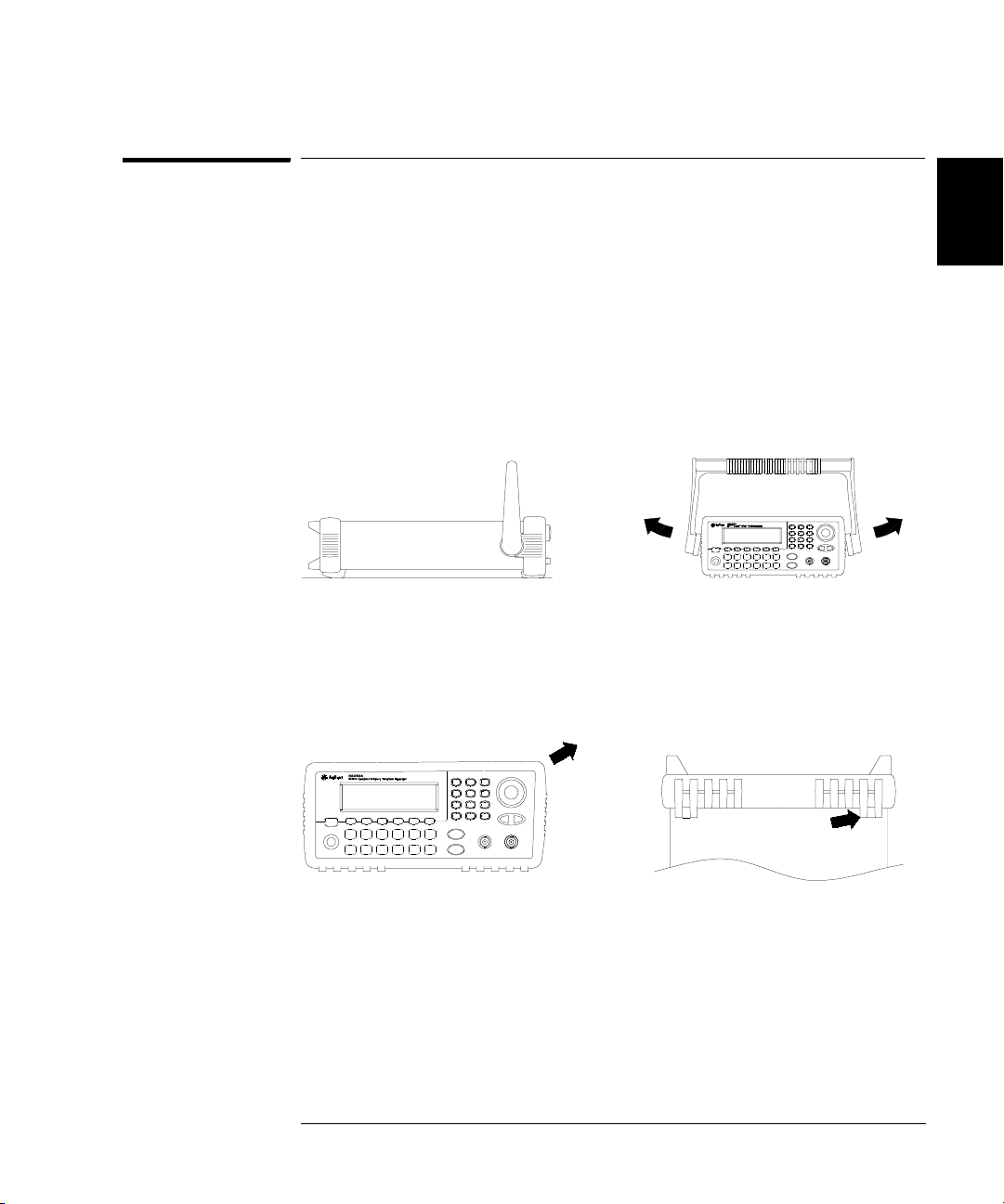
To Adjust the Carrying Handle
2
To adjust the position, grasp the handle by the sides and pull outward.
Then, rotate the handle to the desired position.
Bench-top viewing positions Carrying position
22

To Set the Output Frequency
Chapter 2 Quick Start
To Set the Output Frequency
At power-on, the function generator outputs a sine wave at 1 kHz with
an amplitude of 100 mV peak-to-peak (into a 50Ω termination).
The following steps show you how to change the frequency to 1.2 MHz.
1Press the “Freq” softkey.
The displayed frequency is either the power-on value or the frequency
previously selected. When you change functions, the same frequency is
used if the present value is valid for the new function. To set the
waveform period instead, press the Freq softkey again to toggle to the
Period softkey (the current selection is highlighted).
2 Enter the magnitude of the desired frequency.
Using the numeric keypad, enter the value “1.2”.
2
4
3 Select the desired units.
Press the softkey that corresponds to the desired units. When you select
the units, the function generator outputs a waveform with the displayed
frequency (if the output is enabled). For this example, press MHz
Note: You can also enter the desired value using the knob and arrow keys.
.
23

Chapter 2 Quick Start
To Set the Output Amplitude
To Set the Output Amplitude
2
At power-on, the function generator outputs a sine wave with an
amplitude of 100 mV peak-to-peak (into a 50Ω termination).
The following steps show you how to change the amplitude to 50 mVrms.
1Press the “Ampl” softkey.
The displayed amplitude is either the power-on value or the amplitude
previously selected. When you change functions, the same amplitude is
used if the present value is valid for the new function. To set the amplitude
using a high level and low level, press the Ampl softkey again to toggle to
the HiLevel and LoLevel softkeys (the current selection is highlighted).
2 Enter the magnitude of the desired amplitude.
Using the numeric keypad, enter the value “50”.
3 Select the desired units.
Press the softkey that corresponds to the desired units. When you select
the units, the function generator outputs the waveform with the displayed
amplitude (if the output is enabled). For this example, press mV
Note: You can also enter the desired value using the knob and arrow keys.
24
RMS
.

Chapter 2 Quick Start
To Set the Output Amplitude
You can easily convert the displayed amplitude from one unit to another.
For example, the following steps show you how to convert the amplitude
from Vrms to Vpp.
4 Enter the numeric entry mode.
Press the key to enter the numeric entry mode.
5 Select the new units.
Press the softkey that corresponds to the desired units. The displayed
value is converted to the new units. For this example, press the Vpp
softkey to convert 50 mVrms to its equivalent in volts peak-to-peak.
2
4
To change the displayed amplitude by decades, press the right-arrow
key to move the cursor to the units on the right side of the display.
Then, rotate the knob to increase or decrease the displayed amplitude
by decades.
25

Chapter 2 Quick Start
To Set a DC Offset Voltage
To Set a DC Offset Voltage
2
At power-on, the function generator outputs a sine wave with a dc offset
of 0 volts (into a 50Ω termination). The following steps show you how to
change the offset to –1.5 mVdc.
1Press the “Offset” softkey.
The displayed offset voltage is either the power-on value or the offset
previously selected. When you change functions, the same offset is used
if the present value is valid for the new function.
2 Enter the magnitude of the desired offset.
Using the numeric keypad, enter the value “–1.5”.
3 Select the desired units.
Press the softkey that corresponds to the desired units. When you select
the units, the function generator outputs the waveform with the displayed
offset (if the output is enabled). For this example, press mVdc.
Note: You can also enter the desired value using the knob and arrow keys.
Note: To select dc volts from the front panel, press and then select
the DC On softkey. Press the Offset softkey to enter the desired voltage level.
26

To Set the Duty Cycle
Chapter 2 Quick Start
To Set the Duty Cycle
Applies only to square waves. At power-on, the duty cycle for square
waves if 50%. You can adjust the duty cycle from 20% to 80% for output
frequencies up to 25 MHz. The following steps show you how to change
the duty cycle to 30%.
1 Select the square wave function.
Press the key and then set the desired output frequency to any
value less than 25 MHz.
2Press the “Duty Cycle” softkey.
The displayed duty cycle is either the power-on value or the percentage
previously selected. The duty cycle represents the amount of time per
cycle that the square wave is at a high level (note the icon on the right
side of the display).
3 Enter the desired duty cycle.
Using the numeric keypad or the knob, select a duty cycle value of “30”.
The function generator adjusts the duty cycle immediately and outputs a
square wave with the specified value (if the output is enabled).
2
4
27

Chapter 2 Quick Start
To Configure a Pulse Waveform
To Configure a Pulse Waveform
2
You can configure the function generator to output a pulse waveform
with variable pulse width and edge time. The following steps show you
how to configure a 500 ms pulse waveform with a pulse width of 10 ms
and edge times of 50 µs.
1 Select the pulse function.
Press the key to select the pulse function and output a pulse
waveform with the default parameters.
2 Set the pulse period.
Press the Period softkey and then set the pulse period to 500 ms.
3 Set the pulse width.
Press the Pulse Width softkey and then set the pulse width to 10 ms.
The pulse width represents the time from the 50% threshold of the rising
edge to the 50% threshold of the next falling edge (note the display icon).
4 Set the edge time for both edges.
Press the Edge Time softkey and then set the edge time for both the rising
and falling edges to 50 µs. The edge time represents the time from the
10% threshold to the 90% threshold of each edge (note the display icon).
28

To View a Waveform Graph
Chapter 2 Quick Start
To View a Waveform Graph
In the Graph Mode, you can view a graphical representation of the
current waveform parameters. Each softkey parameter is shown in a
different color corresponding to the lines above the softkeys at the
bottom of the display. Note that the softkeys are listed in the same order
as in the normal display mode.
1 Enable the Graph Mode.
Press the key to enable the Graph Mode. The name of the parameter
currently selected is shown in the upper-left corner of the display and the
numeric value is highlighted.
2 Select the desired parameter.
To select a specific parameter, note the colored bars above the softkeys at
the bottom of the display and select the corresponding color. For example,
to select amplitude, press the softkey below the magenta-colored bar.
• As in the normal display mode, you can edit numbers using the
numeric keypad or the knob and arrow keys.
2
4
• Parameters which normally toggle when you press a key a second time
(e.g., Freq / Period) also toggle in the Graph Mode.
• To exit the Graph Mode, press again.
The key also serves as a key to restore front-panel control
after remote interface operations.
29

Chapter 2 Quick Start
To Output a Stored Arbitrary Waveform
To Output a Stored Arbitrary Waveform
2
There are five built-in arbitrary waveforms stored in non-volatile memory.
The following steps show you how to output the built-in “exponential fall”
waveform from the front panel.
1 Select the arbitrary waveform function.
When you press the key to select the arbitrary waveform function,
a temporary message is displayed indicating which waveform is currently
selected (the default is “exponential rise”).
2 Select the active waveform.
Press the Select Wform softkey and then press the Built-In softkey to
select from the five built-in waveforms. Then press the Exp Fall softkey.
The waveform is output using the present settings for frequency,
amplitude, and offset unless you change them.
The selected waveform is now assigned to the key. Whenever you
press this key, the selected arbitrary waveform is output. To quickly
determine which arbitrary waveform is currently selected, press .
30

To Use the Built-In Help System
To Use the Built-In Help System
Chapter 2 Quick Start
The built-in help system is designed to provide context-sensitive
assistance on any front-panel key or menu softkey. A list of help topics
is also available to assist you with several front-panel operations.
1 View the help information for a function key.
Press and hold down the key. If the message contains more
information than will fit on the display, press the ↓ softkey or turn the
knob clockwise to view the remaining information.
Press DONE to exit the help menu.
2 View the help information for a menu softkey.
Press and hold down the Freq softkey. If the message contains more
information than will fit on the display, press the ↓ softkey or rotate the
knob clockwise to view the remaining information.
2
4
Press DONE to exit the help menu.
31

2
Chapter 2 Quick Start
To Use the Built-In Help System
3 View the list of help topics.
Press the key to view the list of available help topics. To scroll
through the list, press the ↑ or ↓ softkey or rotate the knob. Select the
third topic “Get HELP on any key” and then press SELECT.
Press DONE to exit the help menu.
4 View the help information for displayed messages.
Whenever a limit is exceeded or any other invalid configuration is found,
the function generator will display a message. For example, if you enter
a value that exceeds the frequency limit for the selected function,
a message will be displayed. The built-in help system provides additional
information on the most recent message to be displayed.
Press the key, select the first topic “View the last message displayed”,
and then press SELECT.
Local Language Help: The built-in help system in available in multiple
languages. All messages, context-sensitive help, and help topics appear
in the selected language. The menu softkey labels and status line
messages are not translated.
To select the local language, press the key, press the System
softkey, and then press the Help In softkey. Select the desired language.
32
Chapter 2 Quick Start
To Rack Mount the Function Generator
To Rack Mount the Function Generator
You can mount the Agilent 33250A in a standard 19-inch rack cabinet
using one of two optional kits available. Instructions and mounting
hardware are included with each rack-mounting kit. Any Agilent
System II instrument of the same size can be rack-mounted beside the
Agilent 33250A.
Note: Remove the carrying handle, and the front and rear rubber bumpers,
before rack-mounting the instrument.
To remove the handle, rotate it to vertical and pull the ends outward.
4
2
Front Rear (bottom view)
To remove the rubber bumper, stretch a corner and then slide it off.
33

2
Chapter 2 Quick Start
To Rack Mount the Function Generator
To rack mount a single instrument, order adapter kit 5063-9240.
To rack mount two instruments side-by-side, order lock-link kit 5061-9694
and flange kit 5063-9212. Be sure to use the support rails in the rack cabinet.
In order to prevent overheating, do not block the flow of air into or out of
the instrument. Be sure to allow enough clearance at the rear, sides, and
bottom of the instrument to permit adequate internal airflow.
34

3
3
Front-Panel Menu Operation

3
Front-Panel Menu Operation
This chapter introduces you to the front-panel keys and menu operation.
This chapter does not give a detailed description of every front-panel key
or menu operation. It does, however, give you an overview of the frontpanel menus and many front-panel operations. See the Agilent 33250A
User’s Guide for a complete discussion of the function generator’s
capabilities and operation.
• Front-Panel Menu Reference, on page 37
• To Reset the Function Generator, on page 39
• To Select the Output Termination, on page 39
• To Read the Calibration Information, on page 40
• To Unsecure and Secure for Calibration, on page 41
• To Store the Instrument State, on page 44
• To Configure the Remote Interface, on page 45
36
Chapter 3 Front-Panel Menu Operation
Front-Panel Menu Reference
Front-Panel Menu Reference
This section gives an overview of the front-panel menus. The remainder
of this chapter shows examples of using the front-panel menus.
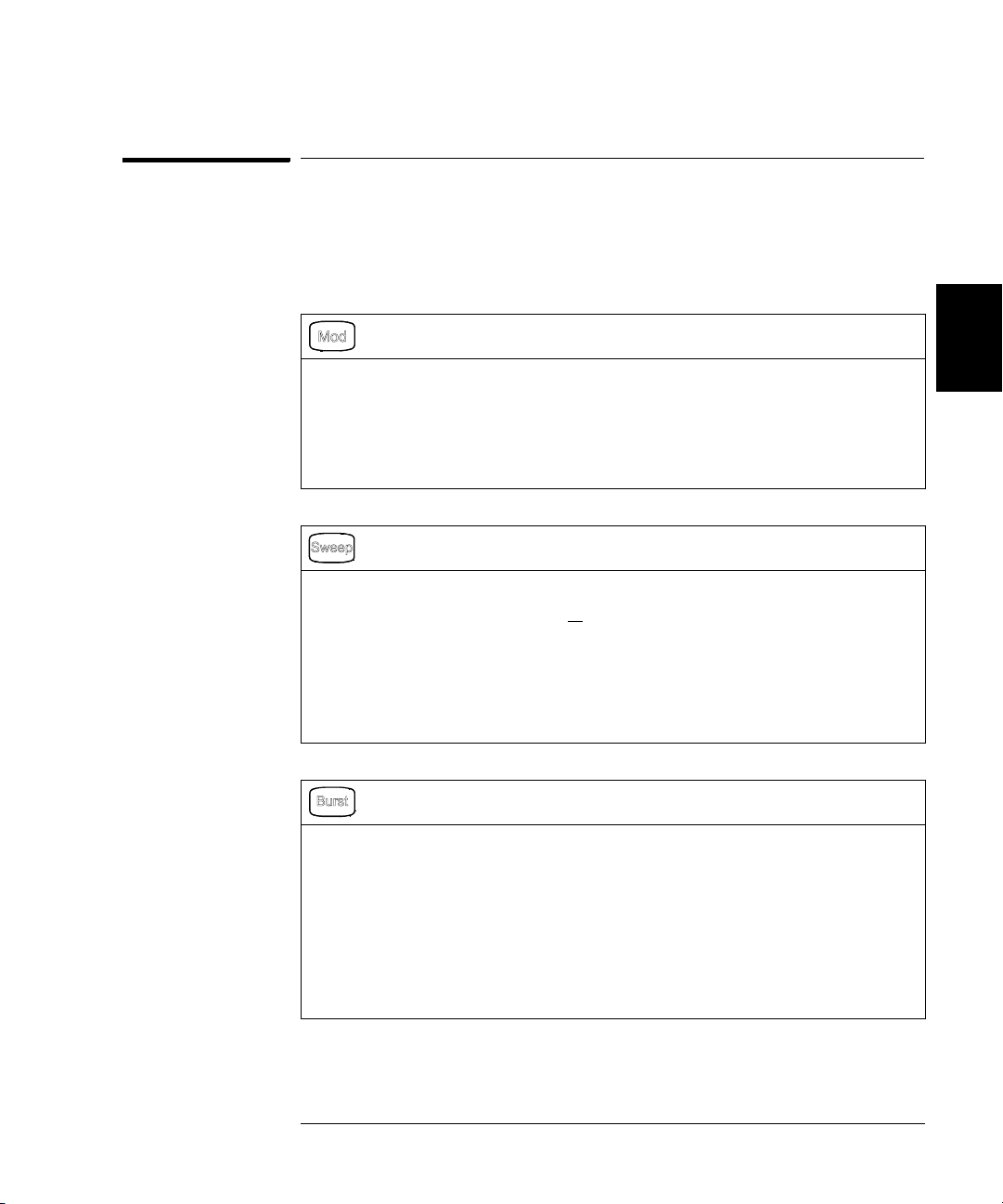
Configure the modulation parameters for AM, FM, and FSK.
• Select the modulation type.
• Select an internal or external modulation source.
• Specify the AM modulation depth, modulating frequency, and modulation shape.
Specify the FM frequency deviation, modulating frequency, and modulation shape.
•
• Specify the FSK “hop” frequency and FSK rate.
Configure the parameters for frequency sweep.
• Select linear or logarithmic sweeping.
• Select the start/stop frequencies or
• Select the time in seconds required to complete a sweep.
• Specify a marker frequency.
• Specify an internal or external trigger source for the sweep.
• Specify the slope (rising or falling edge) for an external trigger source.
• Specify the slope (rising or falling edge) of the “Trig Out” signal.
Configure the parameters for burst.
• Select the triggered (N Cycle) or externally-gated burst mode.
• Select the number of cycles per burst (1 to 1,000,000, or Infinite).
• Select the starting phase angle of the burst (-360° to +360°).
• Specify the time from the start of one burst to the start of the next burst.
• Specify a delay between the trigger and the start of the burst.
• Specify an internal or external trigger source for the burst.
• Specify the slope (rising or falling edge) for an external trigger source.
• Specify the slope (rising or falling edge) of the “Trig Out” signal.
center/ span frequencies.
4
3
37
3
Chapter 3 Front-Panel Menu Operation
Front-Panel Menu Reference
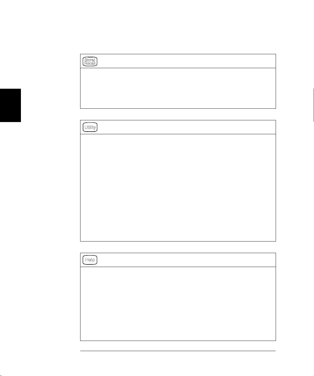
Store and recall instrument states.
• Store up to four instrument states in non-volatile memory.
• Assign a custom name to each storage location.
• Recall stored instrument states.
• Restore all instrument settings to their factory default values.
• Select the instrument’s power-on configuration (last or factory default).
Configure system-related parameters.
• Generate a dc-only voltage level.
• Enable/disable the Sync signal which is output from the “Sync” connector.
• Select the output termination (1Ω to 10 kΩ, or Infinite).
• Enable/disable amplitude autoranging.
• Select the waveform polarity (normal or inverted).
• Select the GPIB address.
• Configure the RS-232 interface (baud rate, parity, and handshake mode).
Select how periods and commas are used in numbers displayed on the front panel.
•
• Select the local language for front-panel messages and help text.
• Enable/disable the tone heard when an error is generated.
• Enable/disable the display bulb-saver mode.
• Adjust the contrast setting of the front-panel display.
• Perform an instrument self-test.
• Secure/unsecure the instrument for calibration and perform manual calibrations.
• Query the instrument’s firmware revision codes.
View the list of Help topics.
• View the last message displayed.
• View the remote command error queue.
• Get HELP on any key.
• How to generate a dc-only voltage level.
• How to generate a modulated waveform.
• How to create an arbitrary waveform.
• How to reset the instrument to its default state.
• How to view a waveform in the Graph Mode.
• How to synchronize multiple instruments.
• How to obtain Agilent Technical Support.
38

Chapter 3 Front-Panel Menu Operation
To Reset the Function Generator
To Reset the Function Generator
To reset the instrument to its factory default state, press and then
select the Set to Defaults softkey. Select YES to confirm the operation.
A complete listing of the instrument’s power-on and reset conditions,
see the “Factory Default Settings” table inside the rear cover of this manual.
To Select the Output Termination
The Agilent 33250A has a fixed series output impedance of 50 ohms to
the front-panel Output connector. If the actual load impedance is
different than the value specified, the displayed amplitude and offset
levels will be incorrect. The load impedance setting is simply provided
as a convenience to ensure that the displayed voltage matches the
expected load.
1Press .
2 Navigate the menu to set the output termination.
Press the Output Setup softkey and then select the Load softkey.
4
3
3 Select the desired output termination.
Use the knob or numeric keypad to select the desired load impedance
or press the Load softkey again to choose “High Z”.
39

3
Chapter 3 Front-Panel Menu Operation
To Read the Calibration Information
To Read the Calibration Information
You can use the instrument’s calibration memory to read the calibration
count and calibration message.
Calibration Count You can query the instrument to determine how
many calibrations have been performed. Note that your instrument was
calibrated before it left the factory. When you receive your instrument,
read the count to determine its initial value. The count value increments
by one for each calibration point, and a complete calibration may
increase the value by many counts.
Calibration Message The instrument allows you to store one message
in calibration memory. For example, you can store such information as
the date when the last calibration was performed, the date when the
next calibration is due, the instrument’s serial number, or even the name
and phone number of the person to contact for a new calibration.
You can record a calibration message only from the remote interface
and only when the instrument is unsecured.
You can read the message from either the front-panel or over the remote
interface. You can read the calibration message whether the instrument
is secured or unsecured.
1 Select the Cal Info interface.
Press and then select the Cal Info softkey from the “Test/Cal” menu.
The first line in the display shows the calibration count.
The second line shows the calibration message.
The last line indicates the current version of the firmware.
The calibration information will time-out and disappear after a few seconds.
Select the Cal Info softkey to show the information again.
2 Exit the menu.
Press the DONE softkey.
40

Chapter 3 Front-Panel Menu Operation
To Unsecure and Secure for Calibration
To Unsecure and Secure for Calibration
This feature allows you to enter a security code to prevent accidental
or unauthorized adjustments of the instrument. When you first receive
your instrument, it is secured. Before you can adjust the instrument,
you must unsecure it by entering the correct security code.
• The security code is set to AT33250A when the instrument is shipped
from the factory. The security code is stored in non-volatile memory,
and does not change when power has been off, after a Factory Reset
(*RST command), or after an Instrument Preset (SYSTem:PRESet
command).
• The security code may contain up to 12 alphanumeric characters.
The first character must be a letter, but the remaining characters
can be letters, numbers, or an underscore ( _ ). You do not have to
use all 12 characters but the first character must always be a letter.
Note: If you forget your security code, you can disable the security feature
by applying a temporary short inside the instrument as described in
“To Unsecure the Instrument Without the Security Code”, on page 69.
4
3
41

3
Chapter 3 Front-Panel Menu Operation
To Unsecure and Secure for Calibration
To Unsecure for Calibration
1 Select the Secure Code interface.
Press and then select the Test/C a l softkey.
2 Enter the Secure Code.
Use the knob to change the displayed character. Use the arrow keys to
move to the next character.
+
When the last character of the secure code is entered, the instrument
will be unsecured.
3 Exit the menu.
Press the DONE softkey.
42

Chapter 3 Front-Panel Menu Operation
To Unsecure and Secure for Calibration
To Secure After Calibration
1 Select the Secure Code interface.
Press and then select the Test/C a l softkey.
2Enter a Secure Code.
Enter up to 12 alphanumeric characters. The first character must be
a letter.
Use the knob to change the displayed character. Use the arrow keys to
move to the next character.
4
3
+
3 Secure the Instrument.
Select the Secure softkey.
4 Exit the menu.
Press the DONE softkey.
43

3
Chapter 3 Front-Panel Menu Operation
To Store the Instrument State
To Store the Instrument State
You can store the instrument state in one of four non-volatile storage
locations. A fifth storage location automatically holds the power-down
configuration of the instrument. When power is restored, the instrument
can automatically return to its state before power-down.
1 Select the desired storage location.
Press and then select the Store State softkey.
2 Select a custom name for the selected location.
If desired, you can assign a custom name to each of the four locations.
• The name can contain up to 12 characters. The first character must
be a letter but the remaining characters can be letters, numbers, or
the underscore character (“_”).
• To add additional characters, press the right-arrow key until the
cursor is to the right of the existing name and then turn the knob.
• To delete all characters to the right of the cursor position, press .
• To use numbers in the name, you can enter them directly from the
numeric keypad. Use the decimal point from the numeric keypad to
add the underscore character (“_” ) to the name.
3 Store the instrument state.
Press the STORE STATE softkey. The instrument stores the selected
function, frequency, amplitude, dc offset, duty cycle, symmetry, as well
as any modulation parameters in use. The instrument does not store
volatile waveforms created in the arbitrary waveform function.
44
Chapter 3 Front-Panel Menu Operation
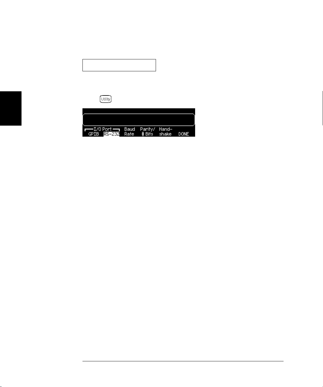
To Configure the Remote Interface
To Configure the Remote Interface
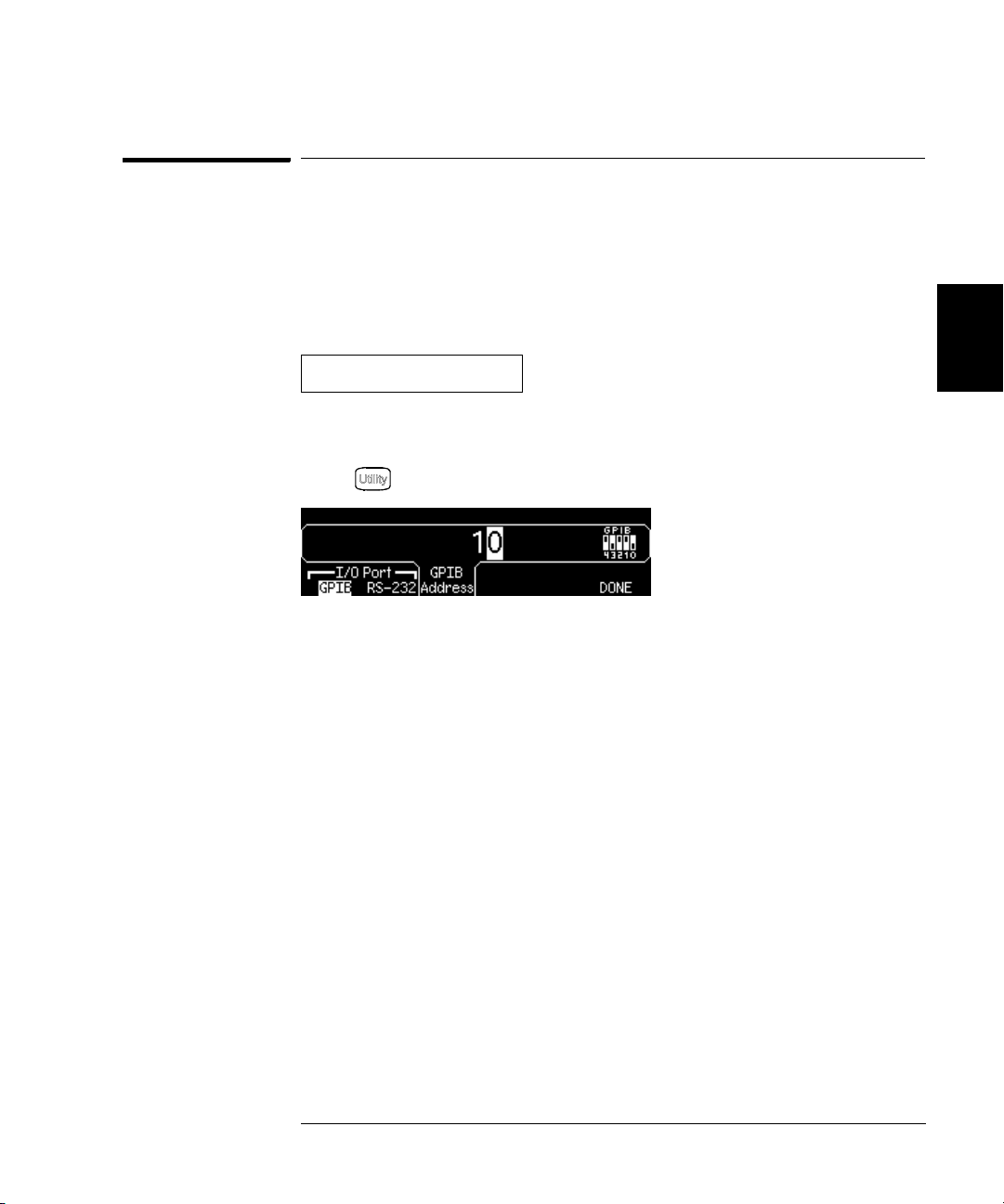
The instrument is shipped with both a GPIB (IEEE-488) interface and an
RS-232 interface. Only one interface can be enabled at a time. The GPIB
interface is selected when the instrument is shipped from the factory.
4
GPIB Configuration
1 Select the GPIB interface.
Press and then select the GPIB softkey from the “I/O” menu.
2 Select the GPIB address.
Press the GPIB Address softkey and enter the desired address using the
numeric keypad or knob. The factory setting is “10”.
The GPIB address is shown on the front-panel display at power-on.
3 Exit the menu.
Press the DONE softkey.
3
45
3
Chapter 3 Front-Panel Menu Operation
To Configure the Remote Interface
RS-232 Configuration
1 Select the RS-232 interface.
Press and then select the RS-232 softkey from the “I/O” menu.
2 Set the baud rate.
Press the Baud Rate softkey and select one of the following:
300, 600, 1200, 2400, 4800, 9600, 19200, 38400, 57600 (factory setting),
or 115200 baud.
3 Select the parity and number of data bits.
Press the Parity / # Bits softkey and select one of the following:
None (8 data bits, factory setting), Even (7 data bits), or Odd (7 data bits).
When you set the parity, you are also setting the number of data bits.
4 Select the handshake mode.
Press the Handshake softkey and select one of the following:
None, DTR /DSR (factory setting), Modem, RTS / CTS, or XON / XOFF.
5 Exit the menu.
Press the DONE softkey.
46

4
4
Calibration Procedures

4
Calibration Procedures
This chapter contains procedures for verification of the instrument’s
performance and adjustment (calibration). The chapter is divided into
the following sections:
• Agilent Technologies Calibration Services, on page 49
• Calibration Interval, on page 50
• Adjustment is Recommended, on page 50
• Time Required for Calibration, on page 51
• Automating Calibration Procedures, on page 52
• Recommended Test Equipment, on page 53
• Test Considerations, on page 54
• Performance Verification Tests, on page 55
• Internal Timebase Verification, on page 60
• AC Amplitude (high-impedance) Verification, on page 61
• Low Frequency Flatness Verification, on page 62
• 0 dB Range Flatness Verification, on page 63
• +10 dB Range Flatness Verification, on page 65
• +20 dB Range Flatness Verification, on page 66
• Calibration Security, on page 68
• Calibration Message, on page 70
• Calibration Count, on page 70
• General Calibration/Adjustment Procedure, on page 71
• Sequence of Adjustments, on page 72
• Aborting a Calibration in Progress, on page 72
• Self-Test, on page 73
• Frequency (Internal Timebase) Adjustment, on page 74
• Internal ADC Adjustment, on page 75
• Output Impedance Adjustment, on page 76
• AC Amplitude (high-impedance) Adjustment, on page 78
• Low Frequency Flatness Adjustment, on page 80
• 0 dB Range Flatness Adjustments, on page 81
• +10 dB Range Flatness Adjustments, on page 83
• +20 dB Range Flatness Adjustment, on page 85
• Pulse Width (Trailing Edge Delay) Adjustment, on page 87
• Pulse Edge Time Adjustment, on page 88
• Duty Cycle Adjustment, on page 89
• Output Amplifier Adjustment (Optional), on page 90
• Calibration Errors, on page 91
48

Chapter 4 Calibration Procedures
Agilent Technologies Calibration Services
Closed-Case Electronic Calibration The instrument features closedcase electronic calibration. No internal mechanical adjustments are
required. The instrument calculates correction factors based upon the
input reference value you set. The new correction factors are stored in
non-volatile memory until the next calibration adjustment is performed.
Non-volatile EEPROM calibration memory does not change when power
has been off or after a remote interface reset.
4
Agilent Technologies Calibration Services
When your instrument is due for calibration, contact your local
Agilent Technologies Service Center for a low-cost recalibration.
The Agilent 33250A is supported on automated calibration systems
which allow Agilent to provide this service at competitive prices.
4
49

Chapter 4 Calibration Procedures
Calibration Interval
Calibration Interval
The instrument should be calibrated on a regular interval determined by
the measurement accuracy requirements of your application. A 1-year
interval is adequate for most applications. Accuracy specifications are
warranted only if adjustment is made at regular calibration intervals.
Accuracy specifications are not warranted beyond the 1-year calibration
interval. Agilent Technologies does not recommend extending calibration
intervals beyond 2 years for any application.
Adjustment is Recommended
4
Whatever calibration interval you select, Agilent Technologies
recommends that complete re-adjustment should always be performed
at the calibration interval. This will assure that the Agilent 33250A
will remain within specification for the next calibration interval.
This criteria for re-adjustment provides the best long-term stability.
Performance data measured using this method can be used to extend
future calibration intervals.
Use the Calibration Count (see page 70) to verify that all adjustments
have been performed.
50
Chapter 4 Calibration Procedures
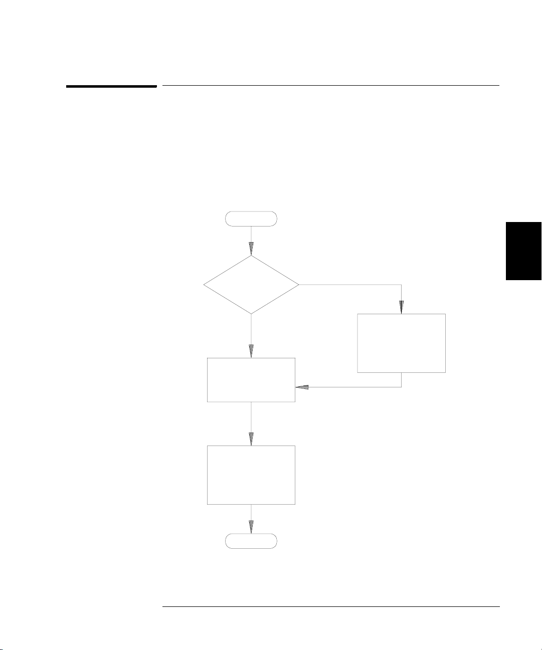
Time Required for Calibration
Time Required for Calibration
The Agilent 33250A can be automatically calibrated under computer control.
With computer control you can perform the complete calibration
procedure and performance verification tests in approximately 30 minutes
once the instrument is warmed-up (see “Test Considerations” on page 54).
Manual adjustments and verifications, using the recommended test
equipment, will take approximately 2 hours.
START
4
Incoming
Verification?
NO
Perform
Adjustments
(approx 1 Hour)
Do Performance
Verification Tests
(approx 1 Hour)
DONE
YES
4
Do Performance
Verification Tests
(approx 1 Hour)
51

4
Chapter 4 Calibration Procedures
Automating Calibration Procedures
Automating Calibration Procedures
You can automate the complete verification and adjustment procedures
outlined in this chapter if you have access to programmable test
equipment. You can program the instrument configurations specified
for each test over the remote interface. You can then enter readback
verification data into a test program and compare the results to the
appropriate test limit values.
You can also adjust the instrument from the remote interface. Remote
adjustment is similar to the local front-panel procedure. You can use a
computer to perform the adjustment by first selecting the required
function and range. The calibration value is sent to the instrument and
then the calibration is initiated over the remote interface. The instrument
must be unsecured prior to initiating the calibration procedure.
For further information on programming the instrument, see chapters
3 and 4 in the Agilent 33250A User’s Guide.
52

Chapter 4 Calibration Procedures
Recommended Test Equipment
Recommended Test Equipment
The test equipment recommended for the performance verification and
adjustment procedures is listed below. If the exact instrument is not
available, substitute calibration standards of equivalent accuracy.
Instrument Requirements Recommended Model Use*
Digital Multimeter
(DMM)
Power Meter 100 kHz to 100 MHz
ac volts, true rms, ac coupled
accuracy: ±0.02% to 1 MHz
dc volts
accuracy: 50 ppm
resolution: 100 µV
Resistance
Offset-compensated
accuracy: ±0.1Ω
1 µW to 100 mW (–30 dBm to +20 dBm)
accuracy: 0.02 dB
resolution: 0.01 dB
Agilent 3458A Q, P, T
Agilent E4418B Q, P, T
4
4
Power Head 100 kHz to 100 MHz
1 µW to 100 mW (–30 dBm to +20 dBm)
Attenuator –20 dB Agilent 8491A Opt 020 Q, P, T
Frequency Meter accuracy: 0.1 ppm Agilent 53131A Opt 010
Oscilloscope 500 MHz
2 Gs/second
50Ω input termination
Adapter N type (m) to BNC (m) N type (m) to BNC (m) Q, P, T
Cable BNC (m) to dual-banana (f) Agilent 10110B Q, P, T
Cable (2 required) Dual banana (m) to dual banana (m) Agilent 11000-60001 Q, P, T
Cable RG58, BNC (m) to dual banana Agilent 11001-60001 Q, P, T
Cable RG58, BNC (m) to BNC (m) Agilent 8120-1840 Q, P, T
* Q = Quick Verification P = Performance Verification
T = Troubleshooting O = Optional Verification
Agilent 8482A Q, P, T
Q, P, T
(high stability)
Agilent 54831B Q, P, T
53

4
Chapter 4 Calibration Procedures
Test Considerations
Test Considerations
For optimum performance, all procedures should comply with the
following recommendations:
• Assure that the calibration ambient temperature is stable and
between 18 °C and 28 °C. Ideally, the calibration should be performed
at 23 °C
• Assure ambient relative humidity is less than 80%.
• Allow a 1-hour warm-up period before verification or adjustment.
• Keep the measurement cables as short as possible, consistent with
the impedance requirements.
• Use only RG-58 or equivalent 50
±1 °C.
Ω cable.
54

Chapter 4 Calibration Procedures
Performance Verification Tests
Performance Verification Tests
Use the Performance Verification Tests to verify the measurement
performance of the instrument. The performance verification tests use
the instrument’s specifications listed in the “Specifications” chapter
beginning on page 13.
You can perform four different levels of performance verification tests:
• Self-Test A series of internal verification tests that give high
confidence that the instrument is operational.
• Quick Verification A combination of the internal self-tests and
selected verification tests.
• Performance Verification Tests An extensive set of tests that are
recommended as an acceptance test when you first receive the
instrument or after performing adjustments.
• Optional Verification Tests Tests not performed with every
calibration. Perform these tests following repairs to the output amplifier.
4
4
55

Chapter 4 Calibration Procedures
Performance Verification Tests
Self-Test
A brief power-on self-test occurs automatically whenever you turn on the
instrument. This limited test assures that the instrument is operational.
To perform a complete self-test:
1 Press on the front panel.
2 Select the Self Test softkey from the “Test/Cal” menu.
A complete description of the self-tests can be found in chapter 6.
The instrument will automatically perform the complete self-test
procedure when you release the key. The self-test will complete in
approximately 30 seconds.
4
• If the self-test is successful, “Self Test Pass” is displayed on the
front panel.
• If the self-test fails, “Self Test Fail” and an error number are displayed.
If repair is required, see chapter 6, “Service,” for further details.
56

Chapter 4 Calibration Procedures
Performance Verification Tests
Quick Performance Check
The quick performance check is a combination of internal self-test and
an abbreviated performance test (specified by the letter
performance verification tests). This test provides a simple method to
achieve high confidence in the instrument’s ability to functionally
operate and meet specifications. These tests represent the absolute
minimum set of performance checks recommended following any service
activity. Auditing the instrument’s performance for the quick check
points (designated by a Q) verifies performance for normal accuracy drift
mechanisms. This test does not check for abnormal component failures.
To perform the quick performance check, do the following:
1 Perform a complete self-test. A procedure is given on page 56.
Q in the
4
2 Perform only the performance verification tests indicated with the
letter Q.
3 If the instrument fails the quick performance check, adjustment or
repair is required.
Performance Verification Tests
The performance verification tests are recommended as acceptance
tests when you first receive the instrument. The acceptance test results
should be compared against the specifications given in chapter 1.
After acceptance, you should repeat the performance verification tests at
every calibration interval.
If the instrument fails performance verification, adjustment or repair
is required.
Adjustment is recommended at every calibration interval. If adjustment
is not made, you must guard band, using no more than 80% of the
specifications listed in chapter 1, as the verification limits.
4
57

4
Chapter 4 Calibration Procedures
Performance Verification Tests
Amplitude and Flatness Verification Procedures
Special Note: Measurements made during the AC Amplitude (highimpedance) Verification procedure (see page 61) are used as reference
measurements in the flatness verification procedures (beginning on
page 62). Additional reference measurements and calculated references
are used in the flatness verification procedures. Photo-copy and use the
table on page 59 to record these reference measurements and perform
the calculations.
The flatness verification procedures use both a DMM and a Power Meter
to make the measurements. To correct the difference between the DMM
and Power Meter measurements, the Power Meter reference measurement
level is adjusted to set the 0.00 dB level to the DMM measurement made
at 1 kHz. The flatness error of the DMM at 100 kHz is used to set the
required 0.00 dB reference.
The instrument internally corrects the difference between the high-Z
input of the DMM and the 50Ω input of the Power Meter when setting
the output level.
The reference measurements must also be converted from Vrms (made
by the DMM) to dBm (made by the Power Meter).
The equation used for the conversion from Vrms (High-Z) to dBm
(at 50Ω) is as follows:
Power (dBm) = 10 log(5.0 * V
Flatness measurements for the –10 dB, –20dB, and –30 dB attenuator
ranges are verified as a part of the 0 dB verification procedure.
No separate verification procedure is given for these ranges.
rms
2
)
58

Chapter 4 Calibration Procedures
Performance Verification Tests
Amplitude and Flatness Verification Worksheet
1. Enter the following measurements (from procedure on page 61).
1kHz_0dB_reference = __________________________ Vrms
1kHz_10dB_reference = __________________________ Vrms
1kHz_20dB_reference = __________________________ Vrms
2. Calculate the dBm value of the rms voltages.
1kHz_0dB_reference_dBm ==10 * log(5.0 * 1kHz_0dB_reference2)
__________________________ dBm
1kHz_10dB_reference_dBm ==10 * log(5.0 * 1kHz_10dB_reference
__________________________ dBm
1kHz_20dB_reference_dBm ==10 * log(5.0 * 1kHz_20dB_reference
__________________________ dBm
2
)
2
)
3. Enter the following measurements (from the procedure on page 62).
100kHz_0dB_reference = __________________________ Vrms
100kHz_10dB_reference = __________________________ Vrms
100kHz_20dB_reference = __________________________ Vrms
4. Calculate the dBm value of the rms voltages.
100kHz_0dB_reference_dBm ==10 * log(5.0 * 100kHz_0dB_reference2)
__________________________ dBm
100kHz_10dB_reference_dBm ==10 * log(5.0 * 100kHz_10dB_reference
__________________________ dBm
100kHz_20dB_reference_dBm ==10 * log(5.0 * 100kHz_20dB_reference
__________________________ dBm
2
)
2
)
5. Calculate the offset values.
4
100kHz_0dB_offset ==100kHz_0dB_reference_dBm – 1kHz_0dB_reference_dBm
__________________________ dBm (use on page 63)
100kHz_10dB_offset ==100kHz_10dB_reference_dBm
__________________________ dBm (use on page 65)
100kHz_20dB_offset ==100kHz_20dB_reference_dBm – 1kHz_20dB_reference_dBm
__________________________ dBm (use on page 66)
– 1kHz_10dB_reference_dBm
59
4
Chapter 4 Calibration Procedures
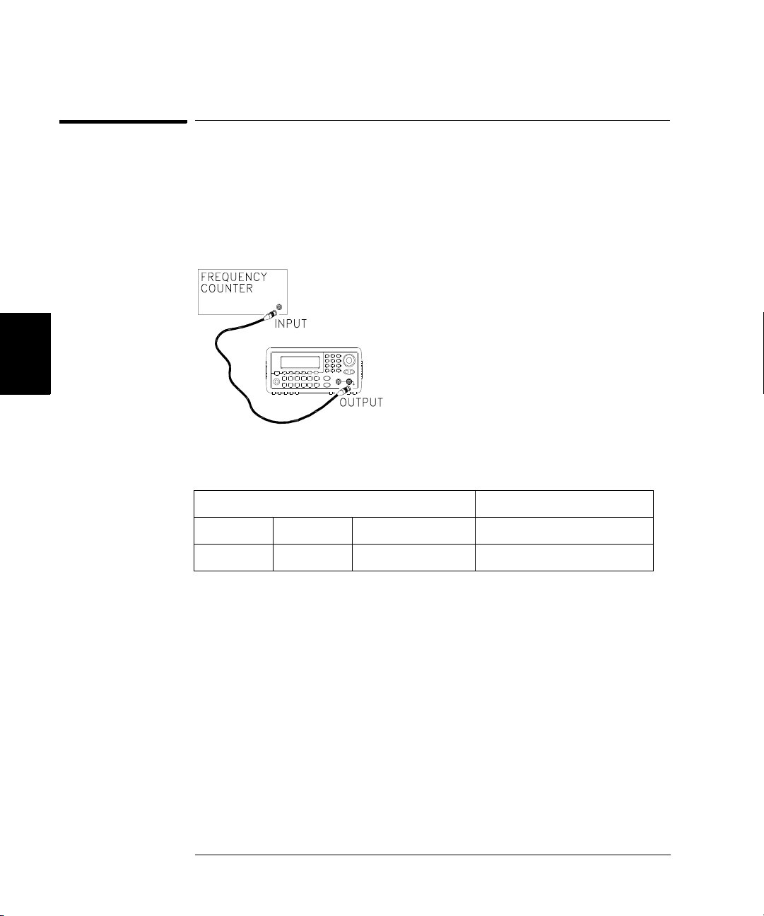
Internal Timebase Verification
Internal Timebase Verification
This test verifies the output frequency accuracy of the instrument.
All output frequencies are derived from a single generated frequency.
1 Connect a frequency counter as shown below (the frequency counter
input should be terminated at 50
Ω).
2 Set the instrument to the output described in the table below and
measure the output frequency. Be sure the instrument output is enabled.
Agilent 33250A Measurement
Function Amplitude Frequency Nominal Error
Q Sine Wave 1.00 Vpp 10.000,000,0 MHz 10.000 MHz ±20 Hz
3 Compare the measured frequency to the test limits shown in the table.
60
Chapter 4 Calibration Procedures
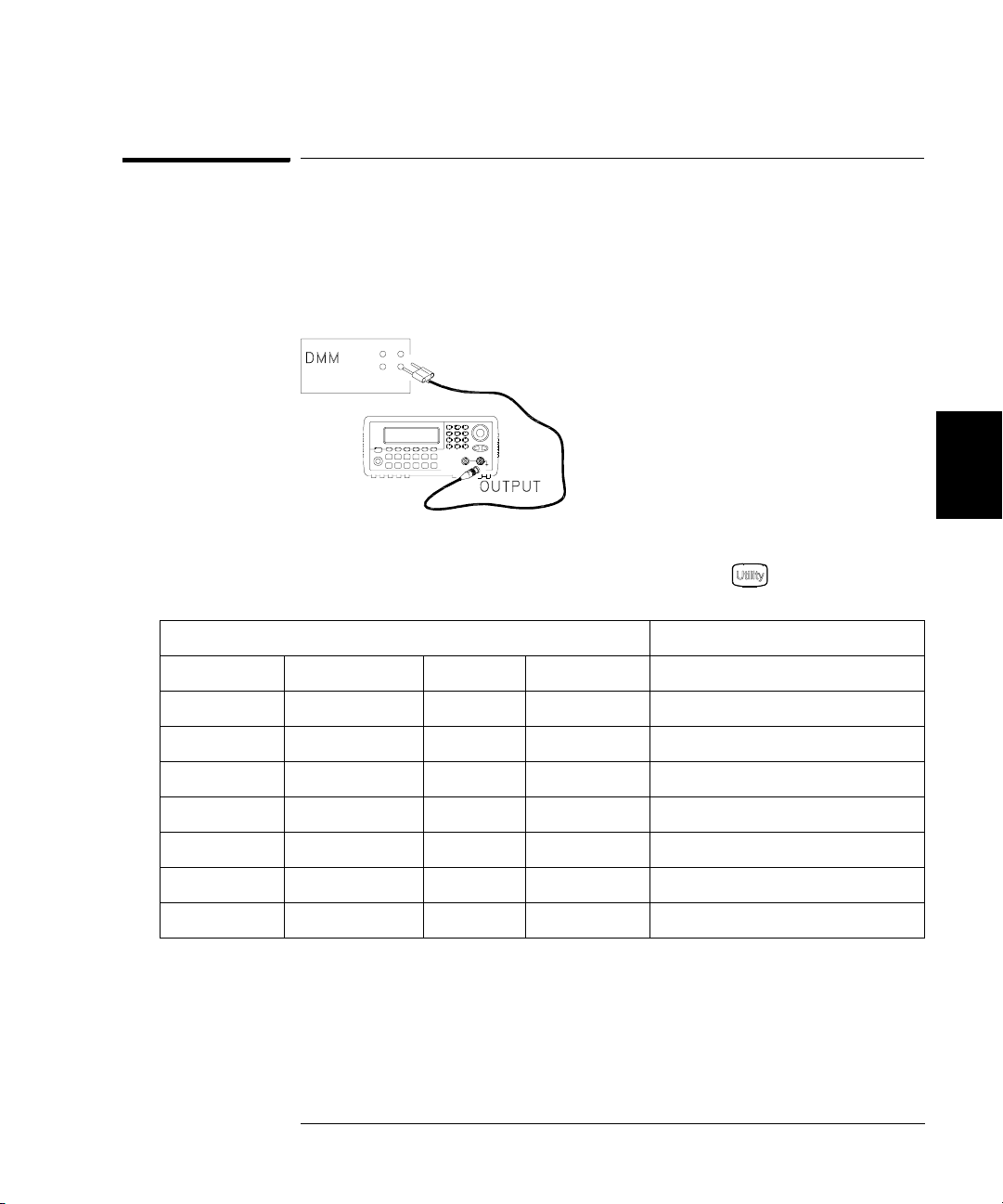
AC Amplitude (high-impedance) Verification
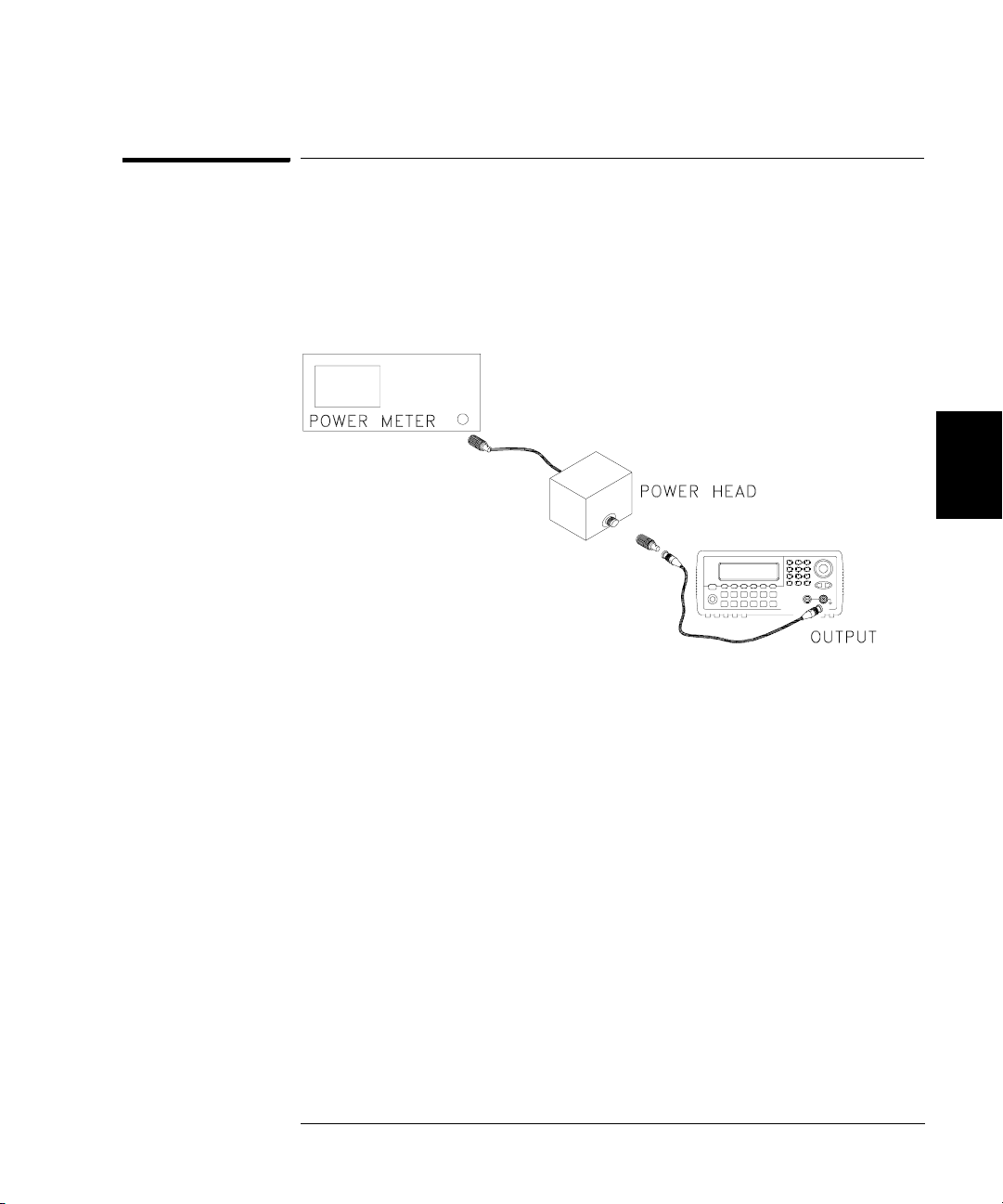
AC Amplitude (high-impedance) Verification
This procedure checks the ac amplitude output accuracy at a frequency
of 1 kHz, and establishes reference measurements for the higher
frequency flatness verification procedures.
1 Set the DMM to measure Vrms Volts. Connect the DMM as shown below.
4
2 Set the instrument to each output described in the table below and
measure the output voltage with the DMM. Press to set the output
impedance to High-Z. Be sure the output is enabled.
4
Agilent 33250A Measurement
Output Setup Function Frequency Amplitude Nominal Error*
Q High Z Sine Wave 1.000 kHz 20.0 mVrms 0.020 Vrms ± 0.00091 Vrms
Q High Z Sine Wave 1.000 kHz 67.0 mVrms 0.067 Vrms ± 0.00138 Vrms
Q High Z Sine Wave 1.000 kHz 200.0 mVrms 0.200 Vrms ± 0.00271 Vrms
1
Q High Z Sine Wave 1.000 kHz 670.0 mVrms 0.670 Vrms
Q High Z Sine Wave 1.000 kHz 2.000 Vrms 2.0000 Vrms 2± 0.0207 Vrms
Q High Z Sine Wave 1.000 kHz 7.000 Vrms 7.000 Vrms
4
Q High Z Square Wave
* Based upon 1% of setting ±1 mVpp (50Ω); converted to Vrms for High-Z.
1
Enter the measured value on the worksheet (page 59) as 1kHz_0dB_reference.
2
Enter the measured value on the worksheet (page 59) as 1kHz_10dB_reference.
3
Enter the measured value on the worksheet (page 59) as 1kHz_20dB_reference.
4
Square wave amplitude accuracy is not specified. This measurement and error
may be used as a guideline for typical operation.
1.000 kHz 900.0 mVrms 0.900 Vrms ± 0.0100 Vrms
± 0.00741 Vrms
3
± 0.0707 Vrms
3 Compare the measured voltage to the test limits shown in the table.
61

4
Chapter 4 Calibration Procedures
Low Frequency Flatness Verification
Low Frequency Flatness Verification
This procedure checks the AC amplitude flatness at 100 kHz using the
reference measurements recorded in the Amplitude and Flatness
Verification Worksheet. These measurements also establish an error value
used to set the power meter reference. The transfer measurements are
made at a frequency of 100 kHz using both the DMM and the power meter.
1 Set the DMM to measure ac Volts. Connect the DMM as shown in the
figure on page 61.
2 Set the instrument to each output described in the table below and
measure the output voltage with the DMM. Press to set the output
impedance to High-Z. Be sure the output is enabled.
Agilent 33250A Measurement
Output Setup Function Frequency Amplitude Nominal Error
Q High Z Sine Wave 100.000 kHz 670.0 mVrms 0.670 Vrms
Q High Z Sine Wave 100.000 kHz 2.0 Vrms 2.000 Vrms
Q High Z Sine Wave 100.000 kHz 7.000 Vrms 7.000 Vrms
1
Enter the measured value on the worksheet (page 59)
as 100kHz_0dB_reference.
2
Enter the measured value on the worksheet (page 59)
as 100kHz_10dB_reference.
3
Enter the measured value on the worksheet (page 59)
as 100kHz_20dB_reference.
1
± 0.0067 Vrms
2
± 0.020 Vrms
3
± 0.070 Vrms
3 Compare the measured voltage to the test limits shown in the table.
4 You have now recorded all the required measurements on the worksheet
(page 59). Complete the worksheet by making all the indicated calculations.
62
Chapter 4 Calibration Procedures
0 dB Range Flatness Verification
0 dB Range Flatness Verification
This procedure checks the high frequency ac amplitude flatness above
100 kHz on the 0 dB attenuator range.
1 Connect the power meter to measure the output amplitude of the
instrument as shown below.
4
4
2 Set the power meter reference level to equal 100kHz_0dB_offset.
This sets the power meter to directly read the flatness error
specification. 100kHz_0dB_offset is calculated on the Amplitude and
Flatness Verification Worksheet.
63

Chapter 4 Calibration Procedures
0 dB Range Flatness Verification
3 Set the instrument to each output described in the table below and
measure the output amplitude with the power meter. Press to set
the output impedance to 50Ω. Be sure the output is enabled.
Agilent 33250A Measurement
Output Setup Function Amplitude Frequency Nominal Error
Q 50 Ω Sine Wave +3.51 dBm 100.000 kHz 0 dB ± 0.086 dB
50 Ω Sine Wave +3.51 dBm 200.000 kHz 0 dB ± 0.086 dB
50 Ω Sine Wave +3.51 dBm 500.000 kHz 0 dB ± 0.086 dB
50 Ω Sine Wave +3.51 dBm 1.500 MHz 0 dB ± 0.086 dB
50 Ω Sine Wave +3.51 dBm 5.000 MHz 0 dB ± 0.086 dB
4
Q 50 Ω Sine Wave +3.51 dBm 10.000 MHz 0 dB ± 0.086 dB
50 Ω Sine Wave +3.51 dBm 25.000 MHz 0 dB ± 0.177 dB
50 Ω Sine Wave +3.51 dBm 40.000 MHz 0 dB ± 0.177 dB
Q 50 Ω Sine Wave +3.51 dBm 50.000 MHz 0 dB ± 0.177 dB
50 Ω Sine Wave +3.51 dBm 60.000 MHz 0 dB ± 0.423 dB
50 Ω Sine Wave +3.51 dBm 65.000 MHz 0 dB ± 0.423 dB
50 Ω Sine Wave +3.51 dBm 70.000 MHz 0 dB ± 0.423 dB
50 Ω Sine Wave +3.51 dBm 75.000 MHz 0 dB ± 0.423 dB
Q 50 Ω Sine Wave +3.51 dBm 80.000 MHz 0 dB ± 0.423 dB
4 Compare the measured output to the test limits shown in the table.
64
Chapter 4 Calibration Procedures
+10 dB Range Flatness Verification
+10 dB Range Flatness Verification
This procedure checks the high frequency ac amplitude flatness above
100 kHz on the +10 dB attenuator range.
1 Connect the power meter to measure the output amplitude of the
instrument as shown on page 63.
2 Set the power meter reference level to equal to the calculated
100kHz_10dB_offset value. This sets the power meter to directly read
the flatness error specification. 100kHz_10dB_offset is calculated on
the Amplitude and Flatness Verification Worksheet.
3 Set the instrument to each output described in the table below and
measure the output amplitude with the power meter. Press to set
the output impedance to 50Ω. Be sure the output is enabled.
Agilent 33250A Measurement
4
4
Output Setup Function Amplitude Frequency Nominal Error
Q 50 Ω Sine Wave +13.00 dBm 100.000 kHz 0 dB ± 0.086 dB
50 Ω Sine Wave +13.00 dBm 200.000 kHz 0 dB ± 0.086 dB
50 Ω Sine Wave +13.00 dBm 500.000 kHz 0 dB ± 0.086 dB
50 Ω Sine Wave +13.00 dBm 1.500 MHz 0 dB ± 0.086 dB
50 Ω Sine Wave +13.00 dBm 5.000 MHz 0 dB ± 0.086 dB
Q 50 Ω Sine Wave +13.00 dBm 10.000 MHz 0 dB ± 0.086 dB
50 Ω Sine Wave +13.00 dBm 25.000 MHz 0 dB ± 0.177 dB
50 Ω Sine Wave +13.00 dBm 40.000 MHz 0 dB ± 0.177 dB
Q 50 Ω Sine Wave +13.00 dBm 50.000 MHz 0 dB ± 0.177 dB
50 Ω Sine Wave +13.00 dBm 60.000 MHz 0 dB ± 0.423 dB
50 Ω Sine Wave +13.00 dBm 65.000 MHz 0 dB ± 0.423 dB
50 Ω Sine Wave +13.00 dBm 70.000 MHz 0 dB ± 0.423 dB
50 Ω Sine Wave +13.00 dBm 75.000 MHz 0 dB ± 0.423 dB
Q 50 Ω Sine Wave +13.00 dBm 80.000 MHz 0 dB ± 0.423 dB
4 Compare the measured output to the test limits shown in the table.
65

4
Chapter 4 Calibration Procedures
+20 dB Range Flatness Verification
+20 dB Range Flatness Verification
This procedure checks the high frequency ac amplitude flatness above
100 kHz on the +20 dB attenuator range.
1 Connect the power meter to measure the output voltage of the
instrument as shown below.
2 Set the power meter reference level to equal to the calculated
100kHz_20dB_offset value. This sets the power meter to directly read the
flatness error specification. 100kHz_20dB_offset is calculated on the
Amplitude and Flatness Verification Worksheet.
Caution Most power meters will require an attenuator or special power head to
measure the +20 dB output.
66

Chapter 4 Calibration Procedures
+20 dB Range Flatness Verification
3 Set the instrument to each output described in the table below and
measure the output amplitude with the power meter. Press to set
the output impedance to 50Ω. Be sure the output is enabled
Agilent 33250A Measurement
Output Setup Function Amplitude Frequency Nominal Error
Q 50 Ω Sine Wave +23.90 dBm 100.000 kHz 0 dB ± 0.086 dB
50 Ω Sine Wave +23.90 dBm 200.000 kHz 0 dB ± 0.086 dB
50 Ω Sine Wave +23.90 dBm 500.000 kHz 0 dB ± 0.086 dB
50 Ω Sine Wave +23.90 dBm 1.500 MHz 0 dB ± 0.086 dB
50 Ω Sine Wave +23.90 dBm 5.000 MHz 0 dB ± 0.086 dB
4
Q 50 Ω Sine Wave +23.90 dBm 10.000 MHz 0 dB ± 0.086 dB
50 Ω Sine Wave +23.90 dBm 25.000 MHz 0 dB ± 0.177 dB
50 Ω Sine Wave +23.90 dBm 40.000 MHz 0 dB ± 0.177 dB
Q 50 Ω Sine Wave +23.90 dBm 50.000 MHz 0 dB ± 0.177 dB
50 Ω Sine Wave +23.90 dBm 60.000 MHz 0 dB ± 0.423 dB
50 Ω Sine Wave +23.90 dBm 65.000 MHz 0 dB ± 0.423 dB
50 Ω Sine Wave +23.90 dBm 70.000 MHz 0 dB ± 0.423 dB
50 Ω Sine Wave +23.90 dBm 75.000 MHz 0 dB ± 0.423 dB
Q 50 Ω Sine Wave +23.90 dBm 80.000 MHz 0 dB ± 0.423 dB
4 Compare the measured output to the test limits shown in the table.
4
67

Chapter 4 Calibration Procedures
Calibration Security
Calibration Security
This feature allows you to enter a security code to prevent accidental
or unauthorized adjustments of the instrument. When you first receive
your instrument, it is secured. Before you can adjust the instrument,
you must unsecure it by entering the correct security code.
See “To Unsecure and Secure for Calibration”, on page 41 for a procedure
to enter the security code.
4
• The security code is set to
from the factory. The security code is stored in non-volatile memory,
and does not change when power has been off, after a Factory Reset
(
*RST command), or after an Instrument Preset (SYSTem:PRESet
command).
• The security code may contain up to 12 alphanumeric characters.
The first character must be a letter, but the remaining characters
can be letters, numbers, or an underscore ( _ ). You do not have to
use all 12 characters but the first character must always be a letter.
Note: If you forget your security code, you can disable the security feature
by applying a temporary short inside the instrument as described on the
following page.
AT33250A when the instrument is shipped
68
Chapter 4 Calibration Procedures
Calibration Security
To Unsecure the Instrument Without the Security Code
To unsecure the instrument without the correct security code, follow the
steps below. See “To Unsecure and Secure for Calibration” on page 41.
See “Electrostatic Discharge (ESD) Precautions” on page 133 before
beginning this procedure.
1 Disconnect the power cord and all input connections.
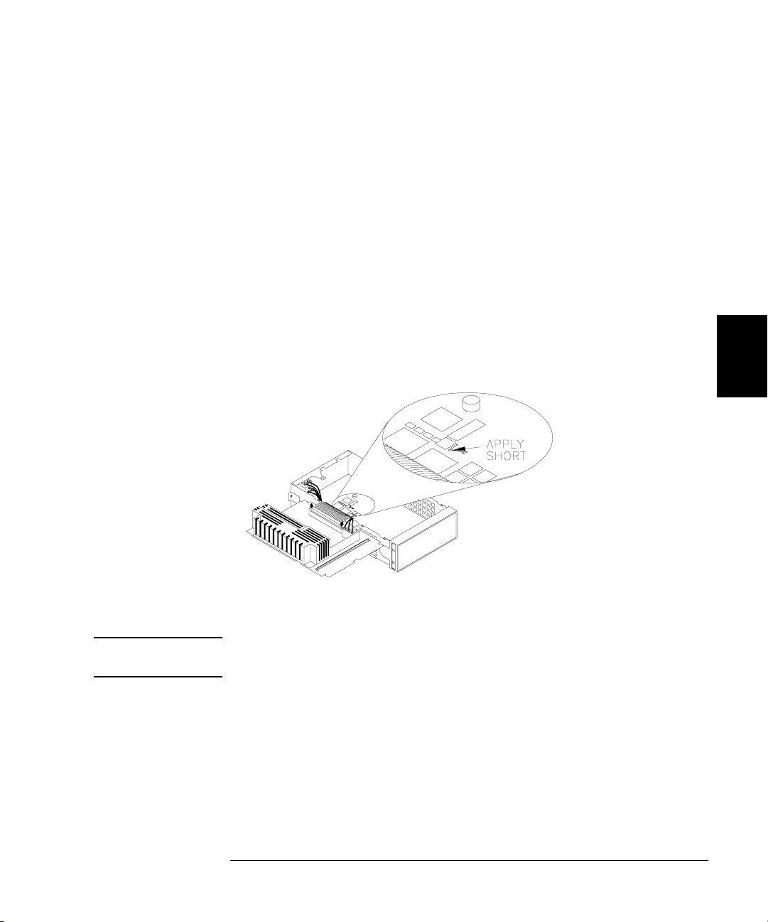
2 Remove the instrument cover. See “Disassembly” on page 140.
3 Remove the main power supply.
4 Apply a temporary short between the two exposed metal pads on the
A1 assembly. The general location is shown in the figure below. On the
PC board, the pads are marked CAL ORIDE.
5 Apply power and turn on the instrument.
WARNING Be careful not to touch the power line connections or high voltages on the
power supply module.
4
4
6 The display will show the message “Calibration security has been
disabled”. The instrument is now unsecured.
7 Turn off the instrument and remove the power cord.
8 Reassemble the instrument.
Now you can enter a new security code, see “To Unsecure and Secure for
Calibration”, on page 41. Be sure you record the new security code.
69

4
Chapter 4 Calibration Procedures
Calibration Message
Calibration Message
The instrument allows you to store one message in calibration memory.
For example, you can store such information as the date when the last
calibration was performed, the date when the next calibration is due,
the instrument’s serial number, or even the name and phone number
of the person to contact for a new calibration.
You can record a calibration message only from the remote interface
and only when the instrument is unsecured.
You can read the message from either the front-panel or over the remote
interface. You can read the calibration message whether the instrument
is secured or unsecured. Reading the calibration message from the front
panel is described on “To Read the Calibration Information”, on page 40.
Calibration Count
You can query the instrument to determine how many calibrations have
been performed. Note that your instrument was calibrated before it left
the factory. When you receive your instrument, read the count to
determine its initial value. The count value increments by one for each
calibration point, and a complete calibration may increase the value by
many counts. See “To Read the Calibration Information”, on page 40.
70

Chapter 4 Calibration Procedures
General Calibration/Adjustment Procedure
General Calibration/Adjustment Procedure
The following procedure is the recommended method to complete an
instrument calibration. This procedure is an overview of the steps
required for a complete calibration. Additional details for each step in
this procedure are given in the appropriate sections of this chapter.
1 Read “Test Considerations” on page 54.
2 Unsecure the instrument for calibration (see page 68).
3 Perform the verification tests, beginning on page page 55, to characterize
the instrument (incoming data).
4 Press on the front panel.
5 Select the “Test / Cal” menu.
6 Select Perform Cal.
7 Enter the Setup Number for the procedure being performed. The default
setup number is “1” and, from the front panel, the number will increment
as the procedures are performed.
8 Select BEGIN.
9 For setups that require an input, adjust the value shown in the display
to the measured value and select ENTER VALUE.
10 The setup will automatically advance to the next required value.
Note To cancel the adjustment procedure, select CANCEL STEP. The display
will return to the setup number entry.
4
4
11 When finished, select END CAL.
12 Secure the instrument against calibration.
13 Note the new security code and calibration count in the instrument’s
maintenance records.
71

4
Chapter 4 Calibration Procedures
Aborting a Calibration in Progress
Aborting a Calibration in Progress
Sometimes it may be necessary to abort a calibration after the procedure
has already been initiated. You can abort a calibration at any time by
turning off the power. When performing a calibration from the remote
interface, you can abort a calibration by issuing a remote interface device
clear message followed by a
The instrument stores calibration constants at the end of each
adjustment procedure. If you lose power, or otherwise abort an
adjustment in progress, you will only need to perform the interrupted
adjustment procedure again.
Caution If you abort a calibration in progress when the instrument is attempting
to write new calibration constants to EEPROM, you may lose all
calibration constants for the function. Typically, upon re-applying power,
the instrument will report error “705 Calibration Aborted”.
*RST.
Sequence of Adjustments
The adjustment sequence shown in the following sections of this chapter
is recommended to minimize the number of test equipment set-up and
connection changes.
You may perform individual adjustments as necessary. Setups 1 through 7
must be performed in order and must be performed before any other
setup procedure.
Note If you have repaired the output amplifier circuitry (U1903, U1904, and
associated components) you should perform the “Output Amplifier
Adjustment (Optional)”, on page 90 before beginning any other
adjustment procedures.
72

Chapter 4 Calibration Procedures
Self-Test
Self-Test
Self-Test is performed as the first step to ensure the instrument is in
working order before beginning any additional adjustments.
1 Press on the front panel. Select Perform Cal on the “Test / Cal”
menu. Enter setup number “1” and select BEGIN.
Setup
1 Performs the Self-test. The Main Output is disabled during test.
2 If the instrument fails any self-test, you must repair the instrument
before continuing the adjustment procedures.
4
4
73

4
Chapter 4 Calibration Procedures
Frequency (Internal Timebase) Adjustment
Frequency (Internal Timebase) Adjustment
The function generator stores a calibration constant that sets the TCXO
to output exactly 10 MHz.
1 Set the frequency counter resolution to better than 0.1 ppm and the
input termination to 50Ω (if your frequency counter does not have a 50Ω
input termination, you must provide an external termination). Make the
connections shown below.
2 Use a frequency counter to measure the output frequency for each setup
in the following table.
Nominal Signal
Setup Frequency Amplitude
2 <10 MHz 1 Vpp Output frequency is slightly less than 10 MHz
3 >10 MHz 1 Vpp Output frequency is slightly more than 10 MHz
4 ~10 MHz 1 Vpp Output frequency should be near 10 MHz
5* 10 MHz 1 Vpp Output frequency should be 10 MHz ±0.5 ppm
* Constants are stored after completing this setup.
3 Using the numerical keypad or knob, adjust the displayed frequency at
each setup to match the measured frequency. Select ENTER VALUE.
4 After performing setup 5:
a. If your calibration procedures require you to verify the adjustment just
made, exit the calibration menu and perform “Internal Timebase
Verification”, on page 60.
b. If you are making all the adjustments and then verifying the instrument’s
performance, continue with the next procedure in this chapter.
74

Chapter 4 Calibration Procedures
Internal ADC Adjustment
Internal ADC Adjustment
The function generator stores calibration constants related to the gain
and offset of the internal ADC. Setup 6 must always be performed
before any other adjustments are attempted. The internal ADC is then
used as a source for the calibration constants generated in setup 7.
1 Make the connections as shown below.
Modulation In
2 Set the DMM to display 5
Record the measurement.
3 Enter the following setup and use the numeric keypad or knob to enter
the measured value of the dc source.
Nominal Signal
½ digits and measure the dc value.
4
4
Setup DC level
6* ~1 Vdc ±10% Calibrates the internal ADC.
* Constants are stored after completing this setup.
4 Disconnect all cables from the rear panel Modulation In connector.
75
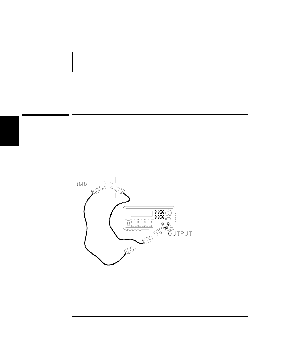
4
Chapter 4 Calibration Procedures
Output Impedance Adjustment
5 Enter and begin the following setup.
Setup
7* Self-calibration. The Main Output is disabled during test.
* Constants are stored after completing this setup.
6 There are no specific operational verification tests for setups 6 and 7
since the constants generated affect almost all behavior of the instrument.
Continue with the next adjustment procedure in this chapter.
Output Impedance Adjustment
The function generator stores calibration constants for the output
impedance. The output impedance constants are generated with and
without the distortion filter and using all five attenuator paths.
1 Set the DMM to measure offset-compensated, four-wire Ohms. Set the
DMM to use 100 NPLC integration. Make the connections as shown below.
76

Chapter 4 Calibration Procedures
Output Impedance Adjustment
2 Use the DMM to make a resistance measurement at the front panel
Output connector for each setup in the following table. The expected
measured value is approximately 50Ω.
Setup
8* -30 dB range with distortion filter
9* -20 dB range with distortion filter
10* -10 dB range with distortion filter
11* 0 dB range with distortion filter
12* +10 dB range with distortion filter
13* -30 dB range without distortion filter
4
14* -20 dB range without distortion filter
15* -10 dB range without distortion filter
16* 0 dB range without distortion filter
17* +10 dB range without distortion filter
* Constants are stored after completing this setup.
3 Using the numeric keypad or knob, adjust the displayed impedance at
each setup to match the measured impedance. Select ENTER VALUE.
4 There are no specific operational verification tests for Output Impedance.
Continue with the next adjustment procedure in this chapter.
4
77
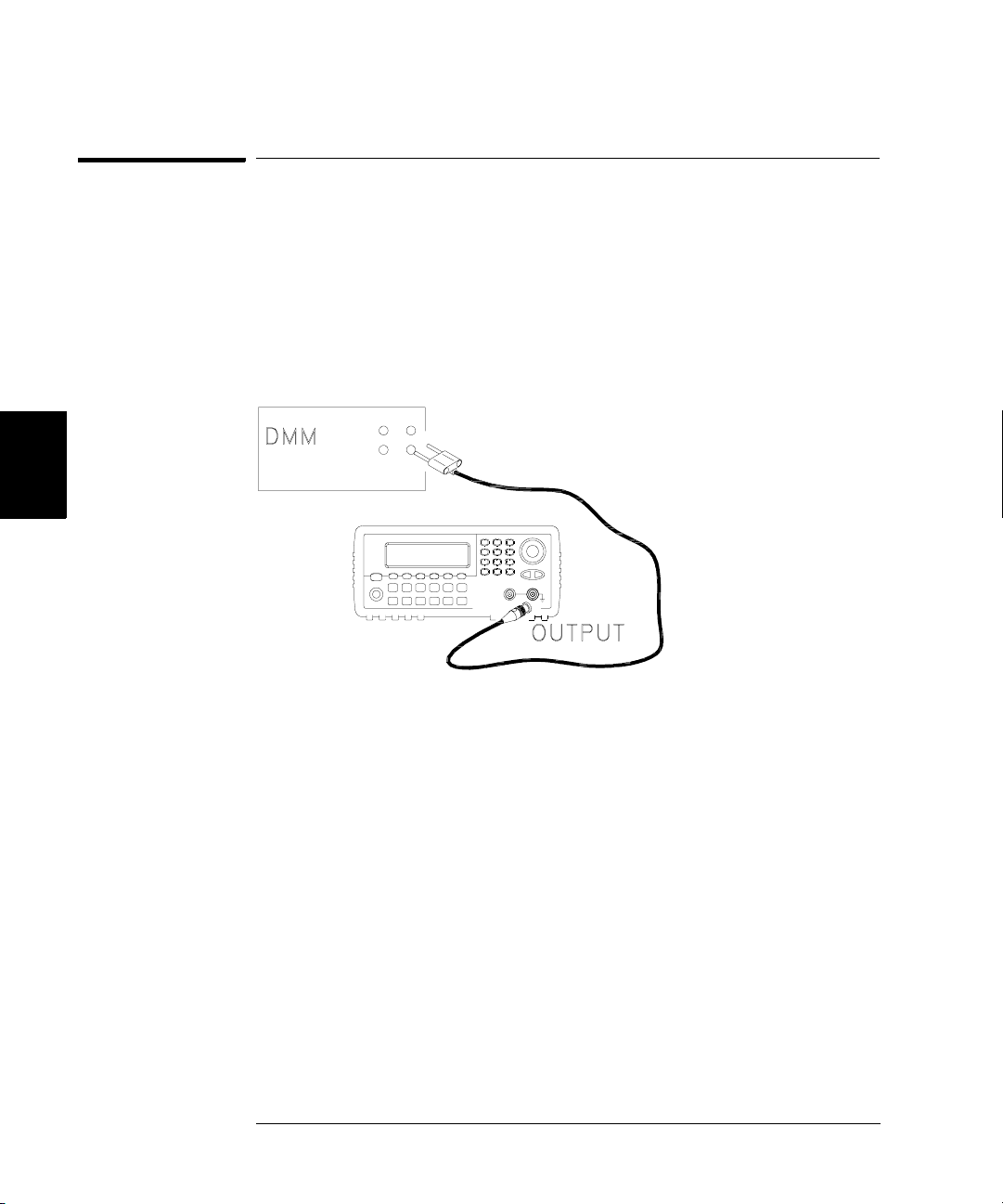
4
Chapter 4 Calibration Procedures
AC Amplitude (high-impedance) Adjustment
AC Amplitude (high-impedance) Adjustment
The function generator stores a calibration constant for each highimpedance attenuator path. The gain coefficient of each path is
calculated using two measurements; one with the waveform DAC at the
+ output and one with waveform DAC at the – output. The setups,
therefore, must be performed in pairs.
1 Connect the DMM as shown below.
78

Chapter 4 Calibration Procedures
AC Amplitude (high-impedance) Adjustment
2 Use the DMM to measure the dc voltage at the front-panel Output
connector for each setup in the following table.
Nominal Signal
Setup DC level
18 +0.015 V Output of -30 dB range
19* -0.015 V Output of -30 dB range
20 +0.05 V Output of -20 dB range
21* -0.05 V Output of -20 dB range
22 +0.15 V Output of -10 dB range
23* -0.15 V Output of -10 dB range
24 +0.50 V Output of 0 dB range
25* -0.50 V Output of 0 dB range
26 +0.15 V Output of -10 dB range (Amplifier In)
27* -0.15 V Output of -10 dB range (Amplifier In)
28 +0.50 V Output of 0 dB range (Amplifier In)
29* -0.50 V Output of 0 dB range (Amplifier In)
30 +1.5 V Output of +10 dB range (Amplifier In)
31* -1.5 V Output of +10 dB range (Amplifier In)
32 +5 V Output of +20 dB range (Amplifier In)
33* -5 V Output of +20 dB range (Amplifier In)
* Constants are stored after completing this setup.
4
4
3 Using the numeric keypad or knob, adjust the displayed voltage at each
setup to match the measured voltage. Select ENTER VALUE. (Entered
values are rounded to the nearest 100 µV.)
4 After performing setup 33:
a. If your calibration procedures require you to verify the adjustment
just made, exit the calibration menu and perform “AC Amplitude (highimpedance) Verification”, on page 61.
b. If you are making all the adjustments and then verifying the instrument’s
performance, continue with the next procedure in this chapter.
79

Chapter 4 Calibration Procedures
Low Frequency Flatness Adjustment
Low Frequency Flatness Adjustment
The Low Frequency Flatness adjustment calculates the flatness response
of 3 attenuator paths with the Elliptical filter and 2 attenuator paths
with the Linear Phase filter.
1 Set the DMM to measure Vrms. Make the connections shown on page 78.
2 Use the DMM to measure the output voltage for each of the setups in the
table below.
Nominal Signal
Setup Frequency Amplitude
4
34* 1 kHz 0.56 Vrms Flatness for 0 dB, Elliptical Filter
35* 100 kHz 0.56 Vrms Flatness for 0 dB, Elliptical Filter
36* 1 kHz 0.56 Vrms Flatness for 0 dB, Linear Phase Filter
37* 100 kHz 0.56 Vrms Flatness for 0 dB, Linear Phase Filter
38* 1 kHz 1.7 Vrms Flatness for +10 dB, Elliptical Filter
39* 100 kHz 1.7 Vrms Flatness for +10 dB, Elliptical Filter
40* 1 kHz 5.6 Vrms Flatness for +20 dB, Elliptical Filter
41* 100 kHz 5.6 Vrms Flatness for +20 dB, Elliptical Filter
42* 1 kHz 5.6 Vrms Flatness for +20 dB, Linear Phase Filter
43* 100 kHz 5.6 Vrms Flatness for +20 dB, Linear Phase Filter
* Constants are stored after completing this setup.
3 Using the numeric keypad or knob, adjust the displayed voltage at each
setup to match the measured voltage. Select ENTER VALUE.
4 After performing setup 43:
a. If your calibration procedures require you to verify the adjustment just
made, exit the calibration menu and perform “Low Frequency Flatness
Verification”, on page 62.
b. If you are making all the adjustments and then verifying the instrument’s
performance, continue with the next procedure in this chapter.
80

Chapter 4 Calibration Procedures
0 dB Range Flatness Adjustments
0 dB Range Flatness Adjustments
1 Connect the power meter as shown on page 83.
2 Use the power meter to measure the output amplitude for each of the
setups in the table below.
Note Setup 44 establishes the power meter reference for all the remaining
setups in this table. You must always perform setup 44 before any of the
following setups.
Nominal Signal
4
Setup Frequency Amplitude
44* 100 kHz 0.28 Vrms 2 dBm Power Meter Reference for 0 dB Range
45* 200 kHz 0.28 Vrms 2 dBm Flatness for 0 dB, Elliptical Filter
46* 500 kHz 0.28 Vrms 2 dBm Flatness for 0 dB, Elliptical Filter
47* 1.5 MHz 0.28 Vrms 2 dBm Flatness for 0 dB, Elliptical Filter
48* 5 MHz 0.28 Vrms 2 dBm Flatness for 0 dB, Elliptical Filter
49* 10.1 MHz 0.28 Vrms 2 dBm Flatness for 0 dB, Elliptical Filter
50* 25.1 MHz 0.28 Vrms 2 dBm Flatness for 0 dB, Elliptical Filter
51* 40.1 MHz 0.28 Vrms 2 dBm Flatness for 0 dB, Elliptical Filter
52* 50.1 MHz 0.28 Vrms 2 dBm Flatness for 0 dB, Elliptical Filter
53* 60.1 MHz 0.28 Vrms 2 dBm Flatness for 0 dB, Elliptical Filter
54* 65.1 MHz 0.28 Vrms 2 dBm Flatness for 0 dB, Elliptical Filter
55* 70.1 MHz 0.28 Vrms 2 dBm Flatness for 0 dB, Elliptical Filter
56* 75.1 MHz 0.28 Vrms 2 dBm Flatness for 0 dB, Elliptical Filter
57* 79.9 MHz 0.28 Vrms 2 dBm Flatness for 0 dB, Elliptical Filter
* Constants are stored after completing this setup.
4
Continued on next page...
81

4
Chapter 4 Calibration Procedures
0 dB Range Flatness Adjustments
Nominal Signal
Setup Frequency Amplitude
58* 200 kHz 0.28 Vrms 2 dBm Flatness for 0 dB, Linear Phase
59* 500 kHz 0.28 Vrms 2 dBm Flatness for 0 dB, Linear Phase
60* 1.5 MHz 0.28 Vrms 2 dBm Flatness for 0 dB, Linear Phase
61* 5 MHz 0.28 Vrms 2 dBm Flatness for 0 dB, Linear Phase
62* 10.1 MHz 0.28 Vrms 2 dBm Flatness for 0 dB, Linear Phase
63* 25.1 MHz 0.28 Vrms 2 dBm Flatness for 0 dB, Linear Phase
64 25.1 MHz 0.15 Vrms –4 dBm Flatness reference measurement
65* 79.9 MHz <0.15 Vrms –4 dBm Flatness high frequency measurement
* Constants are stored after completing this setup.
3 Using the numeric keypad or knob, adjust the displayed amplitude
at each setup to match the measured amplitude (in dBm).
Select ENTER VALUE.
4 After performing setup 65:
a. If your calibration procedures require you to verify the adjustment just
made, exit the calibration menu and perform “0 dB Range Flatness
Verification”, on page 63.
b. If you are making all the adjustments and then verifying the instrument’s
performance, continue with the next procedure in this chapter.
82
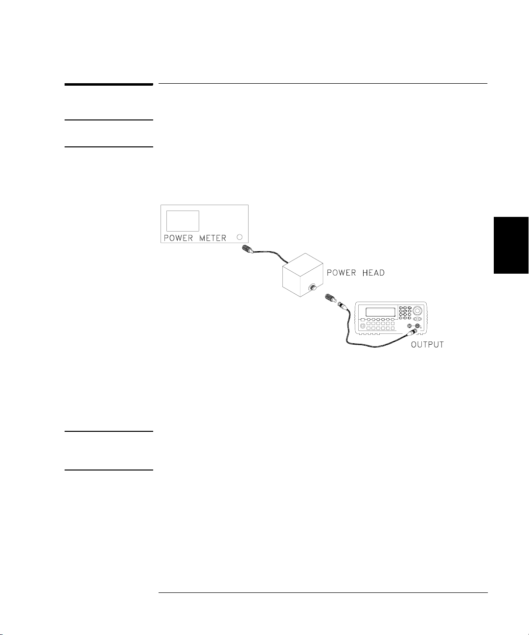
Chapter 4 Calibration Procedures
+10 dB Range Flatness Adjustments
+10 dB Range Flatness Adjustments
Note The Linear Phase path is not adjusted. It is approximated using the other
path’s values.
1 Connect the power meter as shown below.
2 Use the power meter to measure the output amplitude for each of the
setups in the table on the next page.
Note Setup 66 establishes the power meter reference for all the remaining
setups in this table. You must always perform setup 66 before any of
the following setups.
4
4
83

Chapter 4 Calibration Procedures
+10 dB Range Flatness Adjustments
Nominal Signal
Setup Frequency Amplitude
66* 100 kHz 0.9 Vrms 12 dBm Power Meter Reference for +10 dB Range
67* 200 kHz 0.9 Vrms 12 dBm Flatness for +10 dB, Elliptical Filter
68* 500 kHz 0.9 Vrms 12 dBm Flatness for +10 dB, Elliptical Filter
69* 1.5 MHz 0.9 Vrms 12 dBm Flatness for +10 dB, Elliptical Filter
70* 5 MHz 0.9 Vrms 12 dBm Flatness for +10 dB, Elliptical Filter
71* 10.1 MHz 0.9 Vrms 12 dBm Flatness for +10 dB, Elliptical Filter
4
72* 25.1 MHz 0.9 Vrms 12 dBm Flatness for +10 dB, Elliptical Filter
73* 40.1 MHz 0.9 Vrms 12 dBm Flatness for +10 dB, Elliptical Filter
74* 50.1 MHz 0.9 Vrms 12 dBm Flatness for +10 dB, Elliptical Filter
75* 60.1 MHz 0.9 Vrms 12 dBm Flatness for +10 dB, Elliptical Filter
76* 65.1 MHz 0.9 Vrms 12 dBm Flatness for +10 dB, Elliptical Filter
77* 70.1 MHz 0.9 Vrms 12 dBm Flatness for +10 dB, Elliptical Filter
78* 75.1 MHz 0.9 Vrms 12 dBm Flatness for +10 dB, Elliptical Filter
79* 79.9 MHz 0.9 Vrms 12 dBm Flatness for +10 dB, Elliptical Filter
* Constants are stored after completing this setup.
3 Using the numeric keypad or knob, adjust the displayed amplitude at
each setup to match the measured amplitude (in dBm).
Select ENTER VALUE.
4 After performing setup 79:
a. If your calibration procedures require you to verify the adjustment just
made, exit the calibration menu and perform “+10 dB Range Flatness
Verification”, on page 65.
b. If you are making all the adjustments and then verifying the instrument’s
performance, continue with the next procedure in this chapter.
84

Chapter 4 Calibration Procedures
+20 dB Range Flatness Adjustment
+20 dB Range Flatness Adjustment
Caution Most power meters will require an attenuator (-20 dB) or special power
head to measure the +20 dB output.
Be sure to correct the measurements for the specifications of the
attenuator you use. For example, if the nominal attenuator value
is –20 dB at the specified frequency, you must add 20 dB to the power
meter reading before entering the value.
1 Make the connections as shown below.
4
4
2 Use the power meter to measure the output amplitude for each of the
setups in the table on the next page.
Note Setup 80 establishes the power meter reference for all the remaining
setups in this table. You must always perform setup 80 before any of the
following setups.
Nominal Signal
Setup Frequency Amplitude
80* 100 kHz 2.8 Vrms 22 dBm Power Meter Reference
81* 200 kHz 2.8 Vrms 22 dBm Flatness for +20 dB, Elliptical Filter
82* 500 kHz 2.8 Vrms 22 dBm Flatness for +20 dB, Elliptical Filter
83* 1.5 MHz 2.8 Vrms 22 dBm Flatness for +20 dB, Elliptical Filter
* Constants are stored after completing this setup.
Continued on next page...
85

4
Chapter 4 Calibration Procedures
+20 dB Range Flatness Adjustment
Nominal Signal
Setup Frequency Amplitude
84* 5 MHz 2.8 Vrms 22 dBm Flatness for +20 dB, Elliptical Filter
85* 10.1 MHz 2.8 Vrms 22 dBm Flatness for +20 dB, Elliptical Filter
86* 25.1 MHz 2.8 Vrms 22 dBm Flatness for +20 dB, Elliptical Filter
87* 40.1 MHz 2.8 Vrms 22 dBm Flatness for +20 dB, Elliptical Filter
88* 50.1 MHz 2.8 Vrms 22 dBm Flatness for +20 dB, Elliptical Filter
89* 60.1 MHz 2.8 Vrms 22 dBm Flatness for +20 dB, Elliptical Filter
90* 65.1 MHz 2.8 Vrms 22 dBm Flatness for +20 dB, Elliptical Filter
91* 70.1 MHz 2.8 Vrms 22 dBm Flatness for +20 dB, Elliptical Filter
92* 75.1 MHz 2.8 Vrms 22 dBm Flatness for +20 dB, Elliptical Filter
93* 79.9 MHz 2.8 Vrms 22 dBm Flatness for +20 dB, Elliptical Filter
94* 200 kHz 2.8 Vrms 22 dBm Flatness for +20 dB, Linear Phase Filter
95* 500 kHz 2.8 Vrms 22 dBm Flatness for +20 dB, Linear Phase Filter
96* 1.5 MHz 2.8 Vrms 22 dBm Flatness for +20 dB, Linear Phase Filter
97* 5 MHz 2.8 Vrms 22 dBm Flatness for +20 dB, Linear Phase Filter
98* 10.1 MHz 2.8 Vrms 22 dBm Flatness for +20 dB, Linear Phase Filter
99* 25.1 MHz 2.8 Vrms 22 dBm Flatness for +20 dB, Linear Phase Filter
100 60.1 MHz 3.4 Vrms 24 dBm Flatness reference measurement
101* 79.9 MHz ~3.2 Vrms 23 dBm Flatness high frequency measurement
* Constants are stored after completing this setup.
3 Using the numeric keypad or knob, adjust the displayed amplitude at
each setup to match the measured amplitude (in dBm).
Select ENTER VALUE.
4 After performing setup 101:
a. If your calibration procedures require you to verify the adjustment just
made, exit the calibration menu and perform “+20 dB Range Flatness
Verification”, on page 66.
b. If you are making all the adjustments and then verifying the instrument’s
performance, continue with the next procedure in this chapter.
86

Chapter 4 Calibration Procedures
Pulse Width (Trailing Edge Delay) Adjustment
Pulse Width (Trailing Edge Delay) Adjustment
The function generator stores calibration constants used to set the
trailing edge delay (see the discussion on page 110). These setups place
the instrument in pulse mode (at 8 MHz). Setup 102 must be performed
immediately prior to setup 103.
1 Set the oscilloscope to use averaging to determine the pulse width.
Set the oscilloscope to 50Ω input termination (if your oscilloscope
does not have a 50Ω input termination, you must provide an external
termination). Make the connections as shown below.
2 Use the oscilloscope to measure the pulse width of signal at the front-
panel Output terminal for each of the following setups.
Nominal Signal Measurement: Pulse Width(s)
Setup Freq Amplitude Pulse Width
102 8 MHz 1 Vpp 30 ns Narrow pulse width
4
4
103* 8 MHz 1 Vpp 42 ns Wide pulse width
* Constants are stored after completing this setup.
3 Using the numeric keypad or knob, adjust the displayed pulse width at
each setup to match the measured pulse width. Select ENTER VALUE.
4 There are no specific operational verification tests for the Pulse Width
Adjustment. Continue with the next adjustment procedure in this chapter.
87

4
Chapter 4 Calibration Procedures
Pulse Edge Time Adjustment
Pulse Edge Time Adjustment
The function generator stores calibration constants used to calculate the
slope and offset of the edge time DAC outputs. These setups output
100 Hz pulses with 5 ms pulse widths. The setups, following the first
three, must be done in pairs (i.e., 107 immediately before 108).
1 Set the oscilloscope to 50Ω input termination (if your oscilloscope does
not have a 50Ω input termination, you must provide an external
termination). Measure the rise time from the 10% to 90% points on the
waveform. Make the connections shown on page 87.
2 Use an oscilloscope to measure the rise time of the output signal at the
front-panel Output connector for each setup in the following table.
Nominal Signal
Setup Freq Amplitude Rise Time
104 100 Hz 1 Vpp 3.2 ns Fastest transition range 0
105* 100 Hz 1 Vpp 4.5 ns Mid transition range 0
106* 100 Hz 1 Vpp 64 ns Slowest transition range 0
107 100 Hz 1 Vpp 8 ns Fastest transition range 1
108* 100 Hz 1 Vpp 241 ns Slowest transition range 1
109 100 Hz 1 Vpp 161 ns Fastest transition range 2
110* 100 Hz 1 Vpp 4.9 µs Slowest transition range 2
111 100 Hz 1 Vpp 2.6 µs Fastest transition range 3
112* 100 Hz 1 Vpp 82 µs Slowest transition range 3
113 100 Hz 1 Vpp 57 µs Fastest transition range 4
114* 100 Hz 1 Vpp 1.75 ms Slowest transition range 4
* Constants are stored after completing this setup.
1
Rise time measured can vary greatly from the nominal values shown.
1
3 Using the numeric keypad or knob, adjust the displayed rise time
(10% to 90%) at each setup to match the measured rise time.
Select ENTER VALUE.
4 There are no specific operational verification tests for the Pulse Edge Time
Adjustment. Continue with the next adjustment procedure in this chapter.
88

Chapter 4 Calibration Procedures
Duty Cycle Adjustment
Duty Cycle Adjustment
The function generator stores a calibration constant used to calculate
the square wave duty cycle. This setup outputs a 25.1 MHz square wave.
The output frequency in this procedure is chosen to avoid artifacts of
DDS signal generation and internal clock frequencies.
The “Internal ADC Adjustment”, on page 75 must be completed before
doing this procedure.
1 Set the oscilloscope to 50Ω input termination (if your oscilloscope
does not have a 50Ω input termination, you must provide an external
termination). Make the connections shown on page 87.
2 Use an oscilloscope to measure the duty cycle of the signal at the front-
panel Output connector.
Nominal Signal
Setup Freq Amplitude Duty Cycle
115* 25.1 MHz 1 Vpp 50% Enter measured duty cycle
* Constants are stored after completing this setup.
3 Using the numeric keypad or knob, adjust the displayed duty cycle at
each setup to match the measured duty cycle. Select ENTER VALUE.
4 There are no specific operational verification tests for the
Duty Cycle Adjustment.
5 Secure the instrument against further adjustments as described
on page 43.
4
4
You have now completed the recommended adjustment procedures.
You should now verify the output specifications of the instrument using
the “Performance Verification Tests”, on page 55.
89

Chapter 4 Calibration Procedures
Output Amplifier Adjustment (Optional)
Output Amplifier Adjustment (Optional)
This adjustment should only be performed if repairs have been made the
output amplifier circuitry (U1903, U1904, and associated components).
This adjustment is performed at the factory and re-adjustment is not
needed or recommended.
Note You must perform a complete calibration of the instrument following
this adjustment.
1 Disconnect the power cord and all input connections.
2 Remove the instrument cover. See “Disassembly”, on page 140.
4
3 Attach the power cord. Press and hold the “1” button and then turn on
the instrument. Be careful not to touch the power line connections.
4 The display shows a bar graph.
5 Use a long, small, flat-bladed screwdriver to adjust R1959 to minimize
the length of the bar in the display. The adjustment tool can reach R1959
through the slot in the sheet metal as shown.
6 Turn off the instrument and remove the power cord.
7 Re-assemble the instrument.
8 Perform the Adjustment and Verification procedures.
90

Chapter 4 Calibration Procedures
Calibration Errors
Calibration Errors
The following errors are failures that may occur during a calibration.
System error messages are described in chapter 5 of the Agilent 33250A
User’s Guide. Self-test error messages are described in this manual
beginning on page 137.
701 Calibration error; security defeated by hardware jumper
If you short the calibration secure jumper while turning ON the
instrument, this error will occur indicating the security password has
been overwritten.
702 Calibration error; calibration memory is secured
703 Calibration error; calibration memory is secured
704 Calibration error; secure code provided was invalid
705 Calibration error; calibration aborted
706 Calibration error; value out of range
You have typed in a value that was unexpected by the calibration firmware.
For example, if a number is expected such a 50.XX ohms, and you enter
10 ohms, that number is outside the expected range of valid inputs.
707 Calibration error; value out of range
Occurs during the ADC Adjustment, setup 6, if the 1 Volt input voltage is
too high.
850 Calibration error; set up is invalid
You have selected an invalid calibration setup number.
851 Calibration error; set up is out of order
Certain calibration steps require a specific beginning and ending sequence.
You may not enter into the middle of a sequence of calibration steps.
4
4
91

4
92

5
Theory of Operation
5

5
Theory of Operation
This chapter provides descriptions of the circuitry shown on the
schematics in chapter 9.
• Block Diagram, on page 95
• Main Power Supply, on page 97
• On-Board Power Supplies, on page 98
• Waveform DAC and Filters, on page 100
• Digital Waveform, Pulse, and Sync, on page 101
• Digital Waveform Translator, on page 104
• Amplitude Multiplier, on page 106
• Main Output Circuitry, on page 107
• System ADC, on page 110
• System DAC, on page 112
• Synthesis IC, on page 113
• Timebase, on page 115
• Phase Locked Loops, on page 116
• Clock Divider, on page 118
• Trigger and Delay, on page 120
• Waveform RAM, on page 122
• Synchronous Multiplexer, on page 123
• Main Processor, on page 124
• Main Gate Array, on page 125
• DSP and Gateway, on page 126
• Earth-Referenced Logic, on page 126
• Front Panel, on page 127
94

Chapter 5 Theory of Operation
Block Diagram
Block Diagram
A block diagram is shown on the next page. The function generator’s
circuits may be divided into three main categories: power supplies, analog
circuits, and digital circuits. Each portion of the block diagram is
described in the following sections.
The line input voltage is filtered, and then applied to the main power
supply. The main power supply provides all power to the instrument.
Secondary power supplies are contained on the main circuit board.
The secondary supplies control the fan, create the –2.1 V and +3.3 V
voltages, and provide the isolated +5 V supply.
The analog circuitry begins at the Waveform DAC and continues to the
main output. Sine, ramp, noise, and arbitrary waveforms pass directly
from the Waveform DAC to the main output circuitry. Square waves and
pulses are formed in the digital waveform and variable rate edge and
level translation circuits.
The digital circuitry contains all the waveform generation circuitry and
waveform memory. The main CPU and communications CPU (outguard)
are also included.
4
Conventions Used on Schematics and in this Discussion
Major signal and control lines are marked with a name in uppercase.
If the name is followed by an * (for example, TRIG_SYNC*), the line
is inverted logic. If the name is followed by a lowercase e, (for example,
TRIGe), the line is the ECL-level version of a TLL or CMOS signal.
5
95

5
Agilent 33250A Block Diagram
96

Chapter 5 Theory of Operation
Main Power Supply
Power Supplies
The line input voltage is filtered, and then applied to the main power
supply. The main power supply provides all power to the instrument.
Secondary power supplies are contained on the main circuit board.
The secondary supplies control the fan, create the –2.1 V and +3.3 V
voltages, and provide the isolated +5 V supply.
Main Power Supply
The main power supply is a switching supply. No schematic is given for
this supply since it should be replaced as a unit. It features a universal
input, eliminating the need to set power line voltage or frequency.
The main supply provides the following voltages to the main board:
• +5 V (for logic and analog circuitry)
4
• +16 V, –16 V (for analog circuitry)
• –5.2 V (for ECL logic and analog circuitry)
• +12 V isolated (for fan and earth-referenced logic)
• +12 V standby (for power switch and over-temperature shutdown
circuitry)
The main supply uses an electronic power switch, controlled by logic on
the main board, to turn the supplies on or off. The +12 V standby power
is always available when line power is applied. All the power supply
outputs can be checked on the main board.
97
5

5
Chapter 5 Theory of Operation
On-Board Power Supplies
On-Board Power Supplies
See “A1 Power Supply Schematic” on page 204.
The on-board power supply controls the on/off state of the power supply
and conditions the main supplies for use by the analog and digital circuits.
Over-temperature protection is also provided.
The main supply provides a +12 V standby power supply that is used by
the power on/off circuitry. The electronic power switch is controlled by
the PWR_SWITCH* line. This line is grounded when the front-panel
power switch is pushed and turns on Q2004 through R2026.
Pressing the power switch turns on Q2004, and C2043 and C2047 begin
to charge up. Depending upon the state of relay K2001, R2025 will be in
parallel with either R2023 or R2024, so one of the capacitors will charge
much faster than the other. The charged capacitor turns on either Q2006
or Q2008 and energizes the coil of K2001, changing the relay to the
opposite state. Repeatedly pushing the power switch toggles the relay
from one state to the other. In the ON state, PWR_ON* is grounded
through Q2009, turning on the main power supply.
Q2009 can turn off the main supplies if an over-temperature condition is
sensed by U2006, which is powered by the +12 V standby power supply.
U2006 has two trip points for over-temperature. The first trip point is set
at approximately 85 °C and is asserted by OUT 1. This is a warning to
the microprocessor and this condition can be read via GPIB in the status
byte. The second trip point is set at approximately 90 °C and is an actual
over-temperature condition that asserts OUT 2. This turns off Q2009
and shuts off the main supplies.
The actual temperature sensed by U2006 can be read by the microprocessor
through the MEAS_TEMP signal. This reading is used during the
calibration and adjustment process.
Secondary logic supplies are derived from the main power supply’s +5 V
(VCC). Switching regulator U2004 provides the +3.3 V supply (VDD) for
the synthesis IC and waveform memory. U2005 provides the –2.1 V ECL
termination supply (VTT).
The +12 V earth-referenced supply, +12V_ER, is reduced to +5 V by
voltage regulator U2003. This is the earth-referenced logic power supply
(+5_ER).
98

Chapter 5 Theory of Operation
On-Board Power Supplies
The variable-speed fan is driven by a temperature-controlled switching
regulator which is powered by +12V_ER. Comparator U2002-A is
configured as an oscillator whose output (at C2013) is a triangle wave.
Thermistor R2016 senses the incoming air temperature and U2001-A
converts it to a voltage. U2002-B compares this voltage to the triangle
wave and outputs a square wave whose duty cycle varies with temperature.
The square wave is buffered by U104-C and Q2001 and then filtered by
L2003 and C2004 to create a dc voltage that varies with the temperature
and is used to power the fan. Below 30 °C, the fan voltage is set to
approximately 7 volts by R2003 and R2015 (since CR2004 is reversebiased). Above 50 °C, U2001-A’s output voltage is below the minimum
voltage of the triangle wave, keeping Q2001 on constantly and applying
full voltage to the fan.
The PWR_FAIL* line is provided by the main supply to indicate brownout or sagging line input condition. The microprocessor uses this line to
initiate saving the current state of the instrument in non-volatile memory.
4
99
5

5
Chapter 5 Theory of Operation
Waveform DAC and Filters
Analog Circuitry
The analog circuitry begins at the Waveform DAC and continues to the
main output.
Sine, ramp, noise, and arbitrary waveforms pass directly from the
Waveform DAC to the main output circuitry. Square waves and pulses are
formed in the digital waveform and variable-rate level translation circuits.
Waveform DAC and Filters
See “A1 Waveform DAC, Filters, and Comparator Schematic” on page 201.
The 12-bit waveform DAC, U1701, is loaded with data by the
Synchronous Multiplexer of the digital circuitry. The most significant bit
of this data is inverted by U1401-B to convert the 2’s complement value
in memory to the offset-binary representation required by the DAC.
Data is clocked at a 200 MHz rate through differential clock inputs
WFDAC_CLK±. The waveform DAC clock is out of phase with the
LOGIC_CLK to provide ample setup and hold times for the data.
The DAC output, at pins 17 and 18, is centered at –250 mV and ranges
from 0 mV to –500 mV full scale.
Latching relay K1701 connects the DAC output to one of two filters:
•A 9
•A 7
Relay K1701 is driven by the SET_STEP and SET_SINE lines from U306.
The output of the selected filter is applied to amplifier U1703. U1703 has
a gain of 4.3 and the output is level shifted to center at ground potential.
The output ranges from –1.1 V to +1.1 V. U1702 uses VREF (+2.5 V) to
provide an output level appropriate to shift the waveform DAC output to
center around ground.
th
order elliptical filter with a cutoff frequency of 85 MHz.
This filter includes
sine and square waves.
th
order linear-phase filter with a cutoff frequency of 50 MHz. It is
used for ramp, noise, and arbitrary waveforms. It is also used for sine
and square waves in burst mode.
100
sin(x)/x correction. It is used for continuous
 Loading...