Agilent 33220A Service Manual

Download

Service Guide

For safety and warranty information see 

the page immediately after the schematics.

Publication Number 33220-90012 (order as 33220-90100 manual set) Edition 2, March 2005

Agilent 33220A 20 MHz Function/ Arbitrary Waveform Generator

Agilent 33220A at a Glance

The Agilent Technologies 33220A is a 20 MHz synthesized function generator with built-in arbitrary waveform and pulse capabilities. Its combination of bench-top and system features makes this function generator a versatile solution for your testing requirements now and in the future.

Convenient bench-top features

• 10 standard waveforms

• Built-in 14-bit 50 MSa/s arbitrary waveform capability

• Precise pulse waveform capabilities with adjustable edge time

• LCD display provides numeric and graphical views

• Easy-to-use knob and numeric keypad

• Instrument state storage with user-defined names

• Portable, ruggedized case with non-skid feet

Flexible system features

• Four downloadable 64K-point arbitrary waveform memories

• GPIB (IEEE-488), USB, and LAN remote interfaces are standard

• SCPI (Standard Commands for Programmable Instruments) compatibility

Note:

Unless otherwise indicated, this manual applies to all Serial

Numbers.

The Front Panel at a Glance

1 Graph Mode/Local Key 2 On/Off Switch 3 Modulation/Sweep/Burst Keys 4 State Storage Menu Key 5 Utility Menu Key 6 Help Menu Key 7 Menu Operation Softkeys 8 Waveform Selection Keys

9 Manual Trigger Key (used for

Sweep and Burst only)

10 Output Enable/Disable Key 11

Knob

Cursor Keys

Sync Connector

Output Connector

Note: To get context-sensitive help on any front-panel key or menu softkey, press and hold down that key.

The Front-Panel Display at a Glance

Menu Mode

Numeric Readout

Mode

Information

Trigger

Information

Softkey Labels

Units

Output

Status

Graph Mode

To enter or exit the Graph Mode, press the key.

Parameter

Name

Parameter

Value

Display Icon

Signal

Ground

In Graph Mode, only one parameter label is displayed for each key at one time.

Front-Panel Number Entry

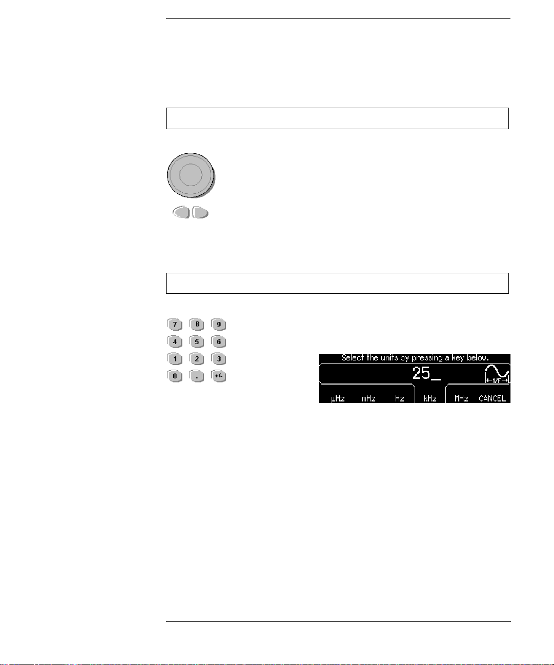
1. Use the keys below the knob to move the cursor left or right.

1. Key in a value as you would on a typical calculator.

You can enter numbers from the front-panel using one of two methods.

Use the knob and cursor keys to modify the displayed number.

2. Rotate the knob to change a digit (clockwise to increase).

Use the keypad to enter numbers and the softkeys to select units.

2. Select a unit to enter the value.

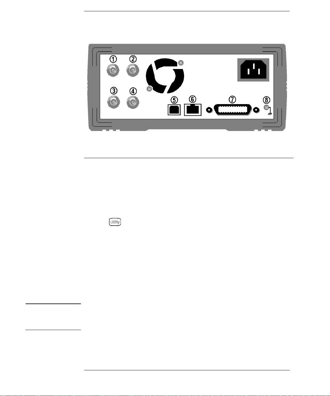
The Rear Panel at a Glance

External 10 MHz Reference Input Terminal (Option 001 only)

Internal 10 MHz Reference Output Terminal (Option 001 only)

3 External Modulation Input Terminal

Input: External Trig/ FSK / Burst Gate

Output: Trigger Output

. .

5 USB Interface Connector 6 LAN Interface Connecto r 7 GPIB Interface Connector 8 Chassis Ground

Use the menu to:

• Select the GPIB address (see chapter 3).

• Set the network parameter s for the LAN interface (see chapter 3).

• Display the current network parameters (see chapter 3).

Note: The External and Internal 10 MHz Reference Terminals (1 and 2, above) are present only if Option 001, External Timebase Reference, is installed. Otherwise, the holes for these connectors are plugged.

WARNING For protection from electrical shock, the power cord ground must not be

defeated. If only a two-contact electrical outlet is available, connect the instrument’s chassis ground screw (see above) to a good earth ground.

In This Book

Specifications Chapter 1 lists the function generator’s specifications.

Quick Start Chapter 2 prepares the function generator for use and

helps you get familiar with a few of its front-panel features.

Front-Panel Menu Operation Chapter 3 introduces you to the frontpanel menu and describes some of the function generator’s menu features.

Calibration Procedures

and adjustment procedures for the

Theory of Operation Chapter 5 describes block and circuit level theory related to the operation of the function generator.

Service Chapter 6 provides guidelines for returning your function generator to Agilent Technologies for servicing, or for servicing it yourself.

Replaceable Parts Chapter 7 contains a detailed parts list of the function generator.

Backdating Chapter 8 describes the differences between this manual and older issues of this manual.

Schematics Chapter 9 contains the function generator’s schematics and component locator drawings.

You can contact Agilent T echnologies at one of the following telephone numbers for warranty, service, or technical support information.

Chapter 4 provides calibration, verification,

function generator.

In the United States: (800) 829-4444 In Europe: 31 20 547 2111 In Japan: 0120-421-345

Or use our Web link for information on contacting Agilent worldwide.

www.agilent.com/find/assist

Or contact your Agilent Technologies Representative.

Chapter 1 Specifications 13 Chapter 2 Quick Start 19

To Prepare the Function Generator for Use 21 To Adjust the Carrying Handle 22 To Set the Output Frequency 23 To Set the Output Amplitude 24 To Set a DC Offset Voltage 26 To Set the High-Level and Low-Level Values 27 To Select “DC Volts” 28 To Set the Duty Cycle of a Square Wave 29 To Configure a Pulse Waveform 30 To View a Waveform Graph 31 To Output a Stored Arbitrary Waveform 32 To Use the Built-In Help System 33 To Rack Mount the Function Generator 35

Chapter 3 Front-Panel Menu Operation 37

Front-Panel Menu Reference 39 To Select the Output Termination 41 To Reset the Function Generator 41 To Read the Calibration Information 42 To Unsecure and Secure for Calibration 43 To Store the Instrument State 46 To Configure the Remote Int erface 47

Contents

Chapter 4 Calibration Procedures 53

Agilent Technologies Calibration Services 55 Calibration Interval 55 Adjustment is Recommended 55 Time Required for Calibration 56 Automating Calibration Procedures 57 Recommended Test Equipment 58 Test Considerations 59 Performance Verification Tests 60 Internal Timebase Verification 64 AC Amplitude (high-impedance) Verification 65 Low Frequency Flatness Verification 66 0 dB Range Flatness Verification 67 +10 dB Range Flatness Verification 69 +20 dB Range Flatness Verification 71 Calibration Security 73 Calibration Message 75 Calibration Count 75 General Calibration/Adjus tment Procedure 76 Aborting a Calibration in Progress 77 Sequence of Adjustments 77 Self-Test 78 Frequency (Internal Timebase) Adjustment 79 Internal ADC Adjustment 80 Output Impedance Adjustment 81 AC Amplitude (high-impedance) Adjustment 83 Low Frequency Flatness Adjustment 85 0 dB Range Flatness Adjustments 86 +10 dB Range Flatness Adjustments 88 +20 dB Range Flatness Adjustment 90 Calibration Errors 93

Chapter 5 Theory of Operation 95

Block Diagram 97 Power Supplies 100 Main Power Supply 100 Earth Referenced Power Supplies 101 Floating Power Supplies 102 Analog Circuitry 103 Waveform DAC and Filters 103 Squarewave Comparator 104 Square and P ulse Level Translator 104 Main Output Circuitry 106 System ADC 107 System DAC 108 Digital Circuitry 110 Synthesis IC and Waveform Memory 110 Timebase, Sync Output, and Relay Drivers 111 Main Processor 112 Front Panel 114 External Timebase (Option 001) 115

Contents

Chapter 6 Service 117

Operating Checklist 118 Types of Service Available 119 Repackaging for Shipment 120 Cleaning 120 Electrostatic Discharge (ESD) Precauti ons 121 Surface Mount Repair 121 Troubleshooting Hi nts 122 Self-Test Procedures 124 Disassembly 127

Chapter 7 Replaceable Parts 139

33220-66511 – Main PC Assembly 141 33220-66502 – Front-Panel PC Assembly 155 33220-66503 – External Timebase PC Assembly 156 33220A Chassis Assembly 158 Manufacturer List 159

Contents

Chapter 8 Backdating 161 Chapter 9 Schematics 163

A1 Clocks, IRQ, RAM, ROM, and USB Schematic 165 A1 Front Panel Interface, LAN, GPIB, and Beeper Schematic 166 A1 Cross Guard, Serial Communications, Non-Volatile Memory, and

Trigger Schematic 167 A1 Power Distribution Schematic 168 A1 Synthesis IC and Wa veform RAM Schematic 169 A1 Timebase, Sync, and Relay Drivers Schematic 170 A1 System ADC Schematic 171 A1 System DAC Schematic 172 A1 Waveform DAC and Filters and Square Wave Comparator Schematic

173 A1 Square / Pulse Level Translation Schematic 174 A1 Gain Switching and Output Amplifier Schematic 175 A1 Earth Referenced Power Supply Schematic 176 A1 Isolated Power Supply S chematic 177 A2 Keyboard Scanner and Display Connector Schematic 178 A2 Key Control Schematic 179 A3 External Timebase Schematic 180 A1 Component Locator (top) 181 A1 Component Locator (bottom) 182 A2 Compone nt Locator 183 A3 Compone nt Locator 184

Specifications

Chapter 1 Specificat ions

Agilent 33220A Function/Arbitrary Waveform Generator

Waveforms

Standard: Sine, Squa re, Ramp,

Built-in Arbitrary: Exponential rise,

Triangle, Pulse, Noise, DC

Exponential fall, Negative ramp, Sin(x)/x, Cardiac.

Waveform Characteristics

Sine

Frequency: 1 µHz to 20 MHz,

Amplitude Flatness:

< 100 kHz 0.1 dB

100 kHz to 5 MHz 0.15 dB

5 MHz to 20 MHz 0.3 dB

Harmonic Distortion:

DC to 20 kHz -70 dBc -70 dBc

20 kHz to 100 kH z -65 dBc -60 dBc

100 kHz to 1 MHz -50 dBc -45 dBc

1 MHz to 20 MHz -40 dBc -35 dBc

Total Harmonic Distortion: DC to 20 kHz 0.04%

Spurious (Non-Harmonic) Output: DC to 1 MHz -70 dBc

1 MHz to 20 MHz -70 dBc +6 dB/octave Phase Noise

(10 kHz offset): -115 dBc / Hz, typical

[1], [2]

[2], [3]

1 µHz resolution

(Relative to 1 kHz)

< 1 Vpp >

[2], [3]

[2], [4]

1 Vpp

Square

Frequency: 1 µHz to 20 MHz,

1 µHz resolution Rise/Fall Time: < 13 ns Overshoot: < 2% Variable Duty Cycle: 20% - 80% (to 10 MHz)

40% - 60% (to 20 MHz) Asymmetry (@ 50% Duty): 1% of period + 5 ns Jitter (RMS): 1 ns + 100 ppm of

period

Ramp, Triangle

Frequency: 1 µHz to 200 kHz,

1 µHz resolution Linearity: < 0.1% of peak output Variable Symmetry: 0.0% to 100.0%

Pulse

Frequency: 500 µHz to 5 MHz,

1 µHz resolution Pulse Width

(period < 10 s): 20 ns minimum,

10 ns resolution Variable Edge Time: < 13 ns to 100 ns

Overshoot: < 2% Jitter (RMS): 300 ps + 0.1 ppm of

period

Noise

Bandwidth: 10 MHz, typical

Arbitrary

Frequency: 1 µHz to 6 MHz,

1 µHz resolution Waveform Length: 2 to 64 K points Amplitude Resolution: 14 bits (including sign) Sample Rate: 50 MSa/s Minimum Rise/Fa ll Time: 35 ns, typical Linearity: < 0.1% of peak output Settling Time: < 250 ns to 0.5% of

final value Jitter (RMS): 6 ns + 30 ppm Non-volatile Memory: Four waveforms

Chapter 1 Specifications

Agilent 33220A Function /Arbitrary Waveform Generator

Common Characteristics

Amplitude

Range:

Into 50 Ω: 10 mVpp to 10 Vpp Into open circuit: 20 mVpp to 20 Vpp

Accuracy (at 1 kHz): Units: Vpp, Vrms, dBm

Resolution: 4 digits

DC Offset

Range (peak AC + DC): ± 5 V into 50 Ω

Accuracy: Resolution: 4 digits

[1], [2]

Main Output

Impedance: 50 Ω typical Isolation: 42 Vpk maximum to

Protection: S hort-circuit prot ected,

Internal Frequency Reference

Accuracy:

[5]

± 10 ppm in 90 days,

External Frequency Reference (Option 001)

Rear Panel Input:

Lock Range: 10 MHz ± 500 Hz Level: 100 mVpp to 5 Vpp Impedance: 1 kΩ typical, AC

Lock Time: < 2 seconds

Rear Panel Output:

Frequency: 10 MHz Level: 632 mVpp (0 dBm),

Impedance: 50 Ω typical, AC

[1], [2]

± 1% of setting

± 1 mVpp

±10 V into open circuit

± 2% of offset setting

± 0.5% of ampl. ± 2 mV

earth overload automatically

disables main output

± 20 ppm in 1 year

coupled

typical coupled

Phase Offset:

Range: +360 to -360 degrees Resolution: 0.001 degrees Accuracy: 20 ns

Modulation

Carrier Waveforms: Sine, Square, Ramp,

Arb Source: Internal/External Internal Modulation: Sine, Square, Ramp,

Triangle, Noise, Arb

(2 mHz to 20 kHz) Depth: 0.0% to 120.0%

Carrier Waveforms: Sine, Square, Ramp,

Arb Source: Internal/External Internal Modulation: Sine, Square, Ramp,

Triangle, Noise, Arb

(2 mHz to 20 kHz) Deviation: DC to 10 MHz

Carrier Waveforms: Sine, Square, Ramp,

Arb Source: Internal/External Internal Modulation: Sine, Square, Ramp,

Triangle, Noise, Arb

(2 mHz to 20 kHz) Deviation: 0.0 to 360.0 degrees

PWM

Carrier Waveforms : Pulse Source: Internal/External Internal Modulation: Sine, Square, Ramp,

Triangle, Noise, Arb

(2 mHz to 20 kHz) Deviation: 0% to 100% of pulse

width

Chapter 1 Specificat ions

Agilent 33220A Function/Arbitrary Waveform Generator

FSK

Carrier Waveforms: Sine, Square, Ramp, Source: Internal/External

Internal Modulation: 50% duty cycle square

External Modulation Input

Arb

(2 mHz to 100 kHz)

[6]

(for AM, FM, PM, PWM)

Voltage Range: ± 5 V full scale Input Resistance: 5 kΩ typical Bandwidth: DC to 20 kHz

Sweep

Waveforms: Sine, Square, Ramp, Type: Linear or Logarithmic

Direction: Up or Down Sweep Time: 1 ms to 500 s Trigger: Single, External or

Marker Falling edge of Sync

Burst

Waveforms: Sine, Square, Ramp,

Type: Counted (1 to 50,000 Start/Stop Phas e: -360 to +360 degrees

Internal Period: 1 µs to 500 s Gate Source: External Trigger Trigger Source: Single, External, or

[7]

Arb

Internal signal (programmable

frequency)

Triangle, Pulse, Noise, Arb

cycles), Infinite, Gated

Internal

T rigger Cha rac teris ti cs

Trigger Input:

Input Level: TTL compatible Slope: Rising or falling,

Pulse Width: > 100 ns Input Impedance: > 10 kΩ, DC coupled Latency: < 500 ns Jitter (RMS) 6 ns (3.5 ns for Pulse)

Trigger Output:

Level: TTL compatible into Pulse Width: > 400 ns

Output Impedance: 50 Ω, typical Maximum Rate: 1 MHz Fanout: <

selectable

1 kΩ

4 Agilent 33220As

Programming Times (typical)

Configuration Times

USB 2.0

Function

Change

Frequency

Change

Amplitude

Change

Select User

Arb

111 m s 111 ms 111 ms

1.5 ms 2.7 ms 1.2 ms

30 ms 30 ms 30 ms

124 ms 124 ms 123 ms

Arb Download Times (binary transfer)

USB 2.0

64 K points 96.9 ms 191.7 ms 336.5 ms 16 K points 24.5 ms 48.4 ms 80.7 ms

4 K points 7.3 ms 14.6 ms 19.8 ms

Download times do not include setup or output time.

LAN

(VXI-11)

LAN

(VXI-11)

GPIB

Chapter 1 Specifications

Agilent 33220A Function /Arbitrary Waveform Generator

General

Power Supply: CAT II

100 to 240 V 50/60 Hz (-5%, +10%)

100 to 120 V @

400 Hz (± 10%) Power Consumption: 50 VA maximum Operating Environment: IEC 61010

Pollution Degree 2

Indoor Location Operating Temperature: 0 °C to 55 °C Operating Humidity: 5% to 80% RH,

non-condensing Operating Altitude: Up to 3000 meters Storage Temperature: -30 °C to 70 °C State Storage Memory: Power off state

automatically sav ed .

Four user-configurabl e

stored states. Interface: GPIB, USB, and LAN

standard Language: SCPI - 1993,

IEEE-488.2 Dimensions (W x H x D):

Bench T op: 261.1 mm by 103.8 mm

by 303.2 mm

Rack Mount: 212.8 mm by 88.3 mm

by 272.3 mm Weight: 3.4 kg (7.5 lbs) Safety Designed to: UL-1244, CSA 1010,

EN61010 EMC Tested to: MIL-461C, EN55011,

EN50082-1 Vibration and Shock: MIL-T-28800, Type III,

Class 5 Acoustic Noise: 30 dBa Warm-up Time: 1 hour

Note: Specifications are subject to change without notice. For the latest specifications, go to the Agilent 33220A product page and find the 33220A Datasheet.

www.agilent.com/find/33220A

This ISM device complie s w ith C ana di an ICES-001. Cet appareil ISM est conforme à la norme NMB-001

du Canada.

N10149

________________

Footnotes:

Add 1/10th of output amplitude and offset

specification per the range of 18

Autorange enabled.

DC offset set to 0 V.

Spurious output at low amplitude is

°C for operation outside

°C to 28 °C.

-75 dBm (typical).

Add 1 ppm / °C (average) for operation out-

side the range of 18

FSK uses trigger input (1 MHz maximum).

Sine and square waveforms above 6 MHz

°C to 28 °C.

are allowed only with an “infinite” burst count.

Product Dimensions

Chapter 1 Specifications

Agilent 33220A Function/Arbitrary Waveform Generator

All dimensions are shown in millimeters.

Quick Start

One of the first things yo u will want to do w ith your function ge nerator is to become acquainted with the fro nt panel. We have w ri tten the exercises in this chapter to prepare the instrument for use and help you get familiar with some of its front-panel operations. This chapter is divided into the following sections:

• To Prepare the Function Generator for Use, on page 21

• To Adjust the Carrying Handle, on page 22

• To Set the Output Frequency, on page 23

• To Set the Output Amplitude, on page 24

• To Set a DC Offset Voltage, on page 26

• To Set the High-Level and Low-Level Values, on page 21

• To Select “DC Volts”, on page 22

• To Set the Duty Cycle of a Square Wave, on page 29

• To Configure a Pulse Waveform, on page 30

• To View a Waveform Graph, on page 31

• To Output a Stored Arbitrary Waveform, on page 32

• To Use the Built-In Help System, on page 33

• To Rack Mount the Function Generator, on page 35

Chapter 2 Quick Start

To Prepare the Function Generator for Use

Power Switch

1 Check the list of supplied items.

Verify that you have received the following items with your instrument. If anything is missing, please contact your nearest Agilent Sales Office.

 One power cord.  One User’s Guide.  This Service Guide.  One folded Quick Start Tutorial.  One folded Quick Reference Guide.  Certificate of Calibration.  Connectivity software on CD-ROM.  One USB 2.0 cable.

2 Connect the power cord and turn on the function generator.

The instrument runs a short power-on self test, which takes a few seconds. When the instrument is ready for use it displays a message about how to obtain help, along with the current GPIB address. The function generator powers up in the sine wave function at 1 kHz with an amplitude of 100 mV peak-to-peak (into a 50Ω termination). the

Output

the key

connector

is disabled. To enable the Output

At power-on,

connector, press

If the function generator does not turn on, verify that the power cord is firmly connected to the power receptacle on the rear p a ne l (t he po w er -line voltage is automatically sensed at power-on). You should also make sure that the function generator is connected to a power source that is energized Then, verify that the function generator is turned on.

If the power-on self test fails, “Self-T est Failed” is displayed along with an error code. See Chapter 6 for information on self-test error codes, and for

instructions on returning the function generator to Agilent for service.

Chapter 2 Quick Start

To Adjust the Carrying Handle

To adjust the position, grasp the handle by the sides and pull outward. Then, rotate the handle to the desired position.

Retracted

Carrying

Position

Extended

To Set the Output Frequency

Chapter 2 Quick Start

To Set the Output Frequency

At power-on, the function generator outputs a sine wave at 1 kHz with an amplitude of 100 mV peak-to-peak (into a 50Ω termination). The following steps show you how to change the frequency to 1.2 MHz.

1Press the “Freq” softkey.

The displayed frequency is either the power-on value or the frequency previously selected. When you change functions, the same frequency is used if the present value is valid for the new function. To set the waveform period instead, press the Freq softkey again to toggle to the Period softkey (the current selection is highlighted).

2 Enter the magnitude of the desired frequency.

Using the numeric keypad, enter the value “1.2”.

3 Select the desired units.

Press the softkey that corresponds to the desired units. When you select the units, the function generator outputs a waveform with the displayed frequency (if the output is enabled). For this example, press MHz

Note: Y keys.

ou can also enter the desired value using the knob and cursor

Chapter 2 Quick Start

To Set the Output Amplitude

At power-on, the function generator outputs a sine wave with an amplitude of 100 mV peak-to-peak (into a 50Ω termination) .

The following steps show you how to change the amplitude to 50 mVrms.

1Press the “Ampl” softkey.

The displayed amplitude is either the power-on value or the amplitude previously selected. When you change functions, the same amplitude is used if the present value is valid for the new function. To set the amplitude using a high level and low level, press the Ampl softkey again to toggle to the HiLevel and LoLevel softkeys (the current selection is highlighted).

2 Enter the magnitude of the desired amplitude.

Using the numeric keypad, enter the value “50”.

3 Select the desired units.

Press the softkey that corresponds to the desired units. When you select the units, the functio n ge ner ator out puts the wave form w ith the disp layed amplitude (if the output is enabled). For this example, press mV

Note: Y keys.

ou can also enter the desired value using the knob and cursor

RMS

Chapter 2 Quick Start

To Set the Output Amplitude

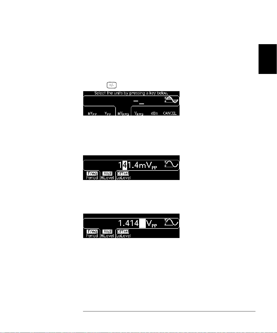
You can easily convert the displayed amplitude from one unit to another. For example, the following steps show you how to convert the amplitude from Vrms to Vpp.

4 Enter the numeric entry mode.

Press the key to enter the numeric entry mode.

5 Select the new units.

Press the softkey that corresponds to the desired units. The displayed value is converted to the new units. For this example, press the Vpp softkey to convert 50 mVrms to its equivalent in volts peak-to-peak.

To change the displayed amplitude by decades, press the right-cursor key to move the cursor to the units on the right side of the display. Then, rotate the knob to increase or decrease the displayed amplitude by decades.

Chapter 2 Quick Start

T o Set a DC Offset Voltage

To Set a DC Offset Voltage

At power-on, the function generator outputs a sine wave with a dc offset of 0 volts (into a 50Ω termination). The following steps show you how to

change the offset to –1.5 mVdc.

1Press the “Offset” softkey.

The displayed off set voltage is either the power-on value or the offset previously selected. When you change functions, the same offset is used if the present value is valid for the new function.

2 Enter the magnitude of the desired offset.

Using the numeric keypad, enter the value “–1.5”.

3 Select the desired units.

Press the softkey that corresponds to the desired units. When you select the units, the functio n ge ner ator out puts the wave form w ith the disp layed offset (if the output is enabled). For this example, press mV

Note: Y keys.

ou can also enter the desired value using the knob and cursor

Chapter 2 Quick Start

To Set the High-Level and Low-Level Values

To Set the High-Level and Lo w-Level Values

You can specify a signal by setting its amplitude and dc offset values, as described previously. Another way to set the limits of a signal is to specify its high-level (maximum) and low-level (minimum) values. This is typically convenient for digital applications. In the following example, let's set the high-level to 1.0 V and the low-level to 0.0 V.

1 Press the "Ampl" softkey to select "Ampl".

2 Press the softkey again to toggle to "HiLevel".

Note that both the Ampl and Offset softkeys toggle together, to HiLevel and LoLevel, respectively.

3 Set the "HiLevel" value.

Using the numeric keypad or the knob, select a value of "1.0 V". (If you are using the keypad, you will need to select the unit, "V", to enter the value.)

4 Press the "LoLevel" softkey and set the value.

Again, use the numeric keyp ad or the knob to enter a value of "0.0 V".

Note that these settings (high-level = "1.0 V" and low-level = "0.0 V") are equivalent to setting an amplitude of "1.0 Vpp" and an offset of "500 mVdc".

Chapter 2 Quick Start

T o Select “DC Volts”

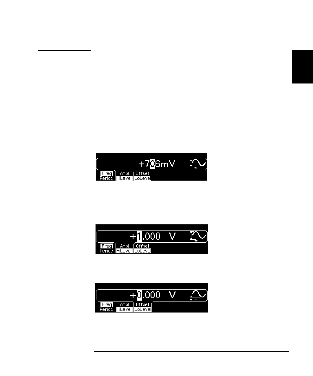
To Select “DC Volts”

You can select the "DC Volts" feature from the “Utility” menu, and then set a constant dc voltage as an "Offset" value. Let's set "DC Volts" = 1.0 Vdc.

1 Press and then select the DC On softkey.

The Offset value becomes selected.

2 Enter the desired voltage level as an "Offset".

Enter 1.0 Vdc with the numeric keypad or knob.

You can enter any dc voltage from -5 Vdc to +5 Vdc.

Chapter 2 Quick Start

T o Set the Duty Cycle of a Square Wave

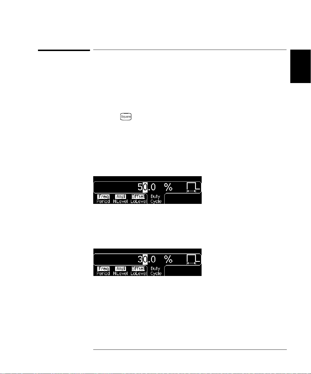
To Set the Duty Cycle of a Square Wave

At power-on, the duty cycle for square waves is 50%. You can adjust th e duty cycle from 20% to 80% for output frequencies up to 10 MHz. The

following steps show you how to change the duty cycle to 30%.

1 Select the square wave function.

Press the key and then set the desired output frequency to any value up to 10 MHz.

2Press the “Duty Cycle” softkey.

The displayed duty cycle is either the power-on value or the percentage previously selected. Th e duty cycle represents the amount of time per cycle that the square wave is at a high level (note the icon on the right side of the display).

3 Enter the desired duty cycle.

Using the numeric keypad or the knob, select a duty cycle value of “30”. The function generator adjusts the duty cy cle immediately and outputs a square wave with the specified value (if the output is enabled).

Chapter 2 Quick Start

T o Configure a Pulse Waveform

To Configure a Pulse Waveform

You can configure the function generator to output a pulse waveform with variable pulse width and edge time. The following steps show you

how to configure a 500 ms pulse waveform with a pulse width of 10 ms and edge times of 50 ns.

1 Select the pulse function.

Press the key to select the pulse function and output a pulse waveform with the default parameters.

2 Set the pulse period.

Press the Period softkey and then set the pulse period to 500 ms.

3 Set the pulse width.

Press the Width softkey and then set the pulse width to 10 ms. The pulse width represents the time from the 50% threshold of the rising edge to the 50% threshold of the next falling edge (note the display icon).

4 Set the edge time for both edges.

Press the Edge Time softkey and then set the edge time for both the rising and falling edges to 50 ns. The edge time represents the time from the 10% threshold to the 90% threshold of each edge (note the display icon

To View a Wav e f o r m Graph

Chapter 2 Quick Start

To View a Waveform Graph

In the Graph Mode, you can view a graphical representation of the current waveform parameters. The softkeys are listed in the same order as in the normal display mode, and they perform the same functions. However, only one label (for example, Freq or Period) is displayed for each softkey at one time.

1 Enable the Graph Mode.

Press the key to enable the Graph Mode. The name of the selected parameter’s numeric value field are both highlighted.

2 Select the desired parame ter.

To select a specific parameter, note the softkey labels at the bottom of the display.

• As in the normal disp lay mode , you can e dit numb ers using either the

parameter,

For example

numeric keypad or the knob and cursor keys.

shown in the up per-left corne r of the display, a nd the

, to select period, press the Period softkey.

currently

•

Param ete rs w h ic h n o rmally toggle wh en you press a key a se cond time also toggle in the Graph Mode. Howev er, you can see on ly on e label for each softkey at one time (for example, Freq or Period).

• To exit the Graph Mode, press again.

The key also serves as a key to restore front-panel control after remote interface operation s.

Chapter 2 Quick Start

To Output a Stored Arbitrary Waveform

There are five built-in arbitrary waveforms stored in non-volatile memory

The following steps show you how to output the built-in “exponential fall” waveform

For information on creating a custom arbitrary waveform, refer to “To Create and Store an Arbitrary Waveform” in the User’s Guide.

1 Select the arbitrary waveform function.

When you press the key to select the arbitrary waveform function, a temporary message is displayed indicating which waveform is currently selected (the default is “exponential rise”).

2 Select the active waveform.

Press the Select Wform softkey and then press the Built-In softkey to select from the five built-in waveforms. Then press the Exp Fall softkey. The waveform is output using the present settings for frequency, amplitude, and offset unless you change them.

from the front panel.

The selected waveform is now assigned to the key. Whenever you press this key, the selected arbitrary waveform is output. To quickly determine which arbitrary waveform is currently selected, press .

To Use the Built-In Help System

Chapter 2 Quick Start

The built-in help system is designed to provide context-sensitive assistance on any front-panel key or menu softkey. A list of help topics is also available to assist you with several front-panel operations.

1 View the help information for a function key.

Press and hold down the key. If the message contains information than will fit on the di spla y, pre s s th e ↓ softkey or turn the knob clockwise to view the remaining information.

Press DONE to exit Help.

2 View the help information for a menu softkey.

Press and hold down the Freq softkey. information than will fit on the di spla y, pre s s th e ↓ softkey or rotate the knob clockwise to view the remaining information.

If the message con tai ns

Press DONE to exit Help.

Chapter 2 Quick Start

To Use the Built-In Help System

3 View the list of help topics.

Press the key to view the list of available help topi cs. To scroll through the list, press the ↑ or ↓ softkey or rotate the knob. Select the third topic “Get HELP on any key” and then press SELECT.

Press DONE to exit Help.

4 View the help information for displayed messages.

Whenever a limit is exceeded or an y other invali d config uration i s found, the function generator will display a message. For example, if you enter a value that exceeds the frequency limit for the selected function, a message will be displayed. The built-in help system provides additional information on the most recent message to be displayed.

Press the k ey, select the first top ic “ and then press SELECT.

Press DONE to exit Help.

Local Language Help: The built-in help system in available in multiple languages. All messages, context-sensitive help, and help topics appear in the selected language. The menu softkey labels and status line messages are not translated.

To select the local language, press the key, press the System softkey, and then press the Help In softkey. Select the desired language.

View the last message displayed”,

Chapter 2 Quick Start

To Rack Mount the Function Generator

You can mount the Agilent 33220A in a standard 19-inch rack cabinet using one of two optional kits available. Instructions and mounting hardware are included with each rack-mounting kit. Any Agilent System II instrument of the same size can be rack-mounted beside the Agilent 33220A.

Note:

before rack-mounting the instrument.

T o remove the handle, rotate it to vertical and pull the ends outward.

Remove the carrying handle, and the front and rear rub ber bumpers

Front

To remove the rubber bumper, stretch a corner and then slide it off.

Rear (bottom view)

Chapter 2 Quick Start

To Rack Mount the Function Generator

T o rack mount a single instrument, order adapter kit 5063-9240.

To rack mount two instruments side-by-side, order lock-link kit 5061-9694 and flange kit 5063-9212. Be sure to use the support rails in the rack cabinet.

Note: The lock-link kit works only for instruments of equal depth. If you want to mount an Agilent 33220A and an instrument of a different depth (for example, an Agilent 33250A) contact your Agilent Representative for further information.

In order to prevent overheating, do not block the flow of air into or out of the instrument. Be sure to allow enough clearance at the rear, sides, and bottom of the instrument to permit adequate internal air flow.

Front-Panel Menu Operation

This chapter introduces you t o the fro nt-pane l keys and menu oper ation. This chapter does not give a deta iled descri ption of eve ry front-pa nel key or menu operation. It does, however, give you an overview of the frontpanel menus and many front-panel operations. Refer to the Agilent 33220A User’s Guide for a complete discussion of the function generator’s capabilities and operation.

• Front-Panel Menu Reference, on page 39

• To Select the Output Termination, on page 41

• To Reset the Function Generator, on page 41

• To Read the Calibration Information, on page 42

• To Unsecure and Secure for Calibration, on page 43

• To Store the Instrument State, on page 46

• To Configure the Remote Interface, on page 47

Chapter 3 Front-Panel Menu Operation

Front-Panel Menu Reference

This section gives an overview of the front-panel menus. The remainder of this chapter contains examples of using the front-panel menus.

Configure the modulation p aramete rs for AM, F M, PM , FSK and PWM.

• Select the modulation type.

• Select an internal or external modulation source.

• Specify AM modulation depth, modulating frequency, and modulation shape. Specify FM frequency deviation, modulating frequency, and modulation shape.

•

Specify PM phase deviation, modulating frequency, and modulation shape.

• Specify FSK “hop” frequency and FSK rate.

• Specify PWM deviation, modulating frequency, and modulation shape.

Configure the parameters for frequency sweep.

• Select linear or logarithmic sweeping.

• Select the start/stop frequencies or

• Select the time in seconds required to complete a sweep.

• Specify a marker frequency.

• Specify an internal or external trigger source for the sweep.

• Specify the slope (rising or falling edge) for an external trigger source.

• Specify the slope (rising or falling edge) of the “Trig Out” signal.

Configure the parameters for burst.

center/span frequencies.

• Select the triggered (N Cycle) or externally-gated burst mode.

• Select the number of cycles per burst (1 to 50,000, or Infinite).

• Select the starting phase angle of the burst (-360° to +360°).

• Specify the time from the start of one burst to the start of the next burst.

• Specify an internal or external trigger source for the burst.

• Specify the slope (rising or falling edge) for an external trigger source.

• Specify the slope (rising or falling edge) of the “Trig Out” signal.

Chapter 3 Front-Panel Menu Operation

Front-Panel Menu Reference

Store and recall instrument states.

• Store up to four instrument states in non-volatile memory.

• Assign a custom name to each storage location.

• Recall stored instrument states.

• Restore all instrument settings to their factory default values.

• Select the instrument’s power-on configuration (last or factory default).

Configure system-related parameters.

• Generate a dc-only voltage level.

• Enable/disable the Sync signal which is output from the “Sync” connector.

• Select the output termination (1Ω to 10 kΩ, or Infinite).

• Enable/disable amplitude autoranging.

• Select the waveform polarity (normal or inverted).

• Select the GPIB address.

• Specify the LAN configuration (IP address and network configuration). Select how periods and commas are used in numbe rs displayed on the front pa nel.

•

• Select the local language for front-panel messages and help text.

• Enable/disable the tone heard when an error is generated.

• Enable/disable the display bulb-saver mode.

• Adjust the contrast setting of the front-panel display.

• Perform an instrument self-test.

• Secure/unsecure the instrument for calibration and perform manual calibrations.

• Query the instrument’s firmware revision codes.

View the list of Help topics.

• View the last message displayed.

• View the remote command error queue.

• Get HELP on any key.

• How to generate a dc-only voltage level.

• How to generate a mo dulated waveform.

• How to create an arbitrary waveform.

• How to reset the instrument to its default state.

• How to view a waveform in the Graph Mode.

• How to synchronize multiple instruments.

• How to obtain Agilent Technical Support.

Chapter 3 Front-Panel Menu Operation

To Select the Output Termination

The Agilent 33220A has a fixed series output impedance of 50 ohms to the front-panel Output connector. If the actual load im pedance is different than the value specified, the displayed amplitude and offset levels will be incorrect. The load impedance setting is simply provided as a convenience to ensure that the displayed voltage matches the expected load.

1Press .

2 Navigate the menu to set the output termination.

Press the Output Setup softkey and then select the Load softkey.

3 Select the desired ou tput termination.

Use the knob or numeric keypad to select the desired load impedance or press the Load softkey again to choose “High Z”.

To Reset the Function Generator

To reset the instrument to its factory default state, press and then select the Set to Defaults softkey. Press YES to confirm the operation.

For a complete listing of the instrument’s power-on and reset conditions, see “Agilent 33220A Factory Default Settings” in the User’s Guide.

Chapter 3 Front-Panel Menu Operation

To Read the Calibration Information

You can access the instrument’s calibration memory to read the calibration count and calibration message.

Calibration Count You can query the instrument to determine how many calibrations have been performed. Note that your instrument was calibrated before it left the factory. When you receive your instrument, read the count to determine its initial value. The count value increments by one for each calibration point, and a complete calibration may increase the value by many counts.

Calibration Message The instrument allows you to store one message in calibration memory. Fo r example, you can s tore the d ate when the last calibration was perfor med, the date wh en th e next calibrat ion is due , the instrument’s serial number, or even the name and phone number of the person to contact for a new calibration.

You can record a calibration message only from the remote interface and only when the instrument is unsecured.

Y ou can read the message from either the front-panel or over the remote interface. You can read the calibration message whether the instrument is secured or unsecured.

1 Select the Cal Info interface.

Press and then select the Cal Info softkey from the “Test/Cal” menu. The first line in the display shows th e calibration count.

The second line shows the calibration message. The last line indicates the current version of the firmware.

The calibration info rmation will tim e-out and disappea r after a few sec onds. Select the Cal Info softkey to show t he inf orma tio n agai n.

2 Exit the menu.

Press the DONE softkey.

Chapter 3 Front-Panel Menu Operation

T o Unsecure and Secure for Calibration

To Unsecure and Secure for Calibration

This feature allows you to enter a security code to prevent accidental or unauthorized adjustments of the instrument. When you first receive your instrument, it is secured. Before you can adjust the instrument, you must unsecure it by entering the correct security code.

• The security code is set to AT33220A when the instrument is shipped from the factory. The security code is stored in non-volatile memory, and does not change when power has been off, after a Factory Reset (*RST command), or after an Instrument Preset (SYSTem:PRESet command).

• The security code may contain up to 12 alphanumeric characters. The first character must be a letter, but the remaining characters can be letters, numbers, or an underscore ( _ ). You do not have to use all 12 characters but the first character must always be a letter.

Note If you forget your security code, you can disable the security feature by

applying a temporary short inside the instrument as described in “To Unsecure the Instrument Without the Security Code” on page 73.

Chapter 3 Front-Panel Menu Operation

To Unsecure and Secure for Calibration

To Unsecure for Calibration

1 Select the Secure Code interface.

Press and then select the Test/Cal softkey.

2 Enter the Secure Code.

Use the knob to change the displayed character. Use the arrow keys to move to the next character.

When the last character of the secure code is entered, the instrument will be unsecured.

3 Exit the menu.

Press the DONE softkey.

Chapter 3 Front-Panel Menu Operation

T o Unsecure and Secure for Calibration

To Secure After Calibration

1 Select the Secure Code interface.

Press and then select the Test/Cal softkey.

2Enter a Secure Code.

Enter up to 12 alphanumeric characters. The first character must be a letter.

Use the knob to change the displayed character. Use the arrow keys to move to the next character.

3 Secure the Instrument.

Select the Secure softkey.

4 Exit the menu.

Press the DONE softkey.

Chapter 3 Front-Panel Menu Operation

T o Store the Instrument State

To Store the Instrument State

You can store the instrument state in one of four non-volatile storage locations. A fifth storage location automatically holds the power-down configuration of the instrument. When power is restored, the instrument can automatically return to its state before power-down.

1 Select the desired storage location.

Press and then select the Store State softkey.

2 Select a custom name for the selected location.

If desired, you can assign a custom name to each of the four locations.

• The name can contain up to 12 characters. The first character be a letter but the remaining characters can be letters, numbers the underscore character (“_”).

• To add additional characters, press the right-cursor key until the cursor is to the right of the existing name and then turn the knob.

• To delete all characters to the right of the cursor position, press .

• To use numbers in the name, you can enter them directly from the numeric keypad. Use the de cimal point from the numeric keypad to add the underscore character (“_”) to the name.

3 Store the instrument state.

Press the STORE STATE softkey. The instrument stores the selected function, frequency, amplitude, dc offset, duty cycle, symmetry, as well as any modulation parameters in use. The instrument does not store volatile waveforms created in the arbitrary waveform function.

must

, or

Chapter 3 Front-Panel Menu Operation

To Configure the Remote Interface

The Agilent 33220A supports remote interface communication using a choice of three interfaces: GPIB, USB, and LAN. All three interfaces are "live" at power up. The instructions that follow tell how to conf igure y our remote interface from the instrument front panel.

Note Connectivity software is provided with your instrument on CD-ROM to

enable communications over these interfaces. Install this software as described in the instructions provided with the CD-ROM.

GPIB Configuration

You need only select a GPIB address.

1 Select the “I/O” menu.

Press and then press the

2 Select the GPIB address.

Use the knob and cursor keys or the numeric keypad to select a GPIB address in the range 0 through 30 (the factory default is “10”).

The GPIB address is shown on the front-panel display at power-on.

3 Exit the menu.

I/O softkey.

Press the DONE softkey.

USB Configuration

The USB interface requires no front panel configuration parameters. Just connect the Agilent 33220A to your PC with the appropriate USB cable. The interface will self configure. Press the Show USB Id softkey in the “I/O menu” to see the USB interface identification string. Both USB

1.1 and USB 2.0 are supported.

Chapter 3 Front-Panel Menu Operation

To Configure the Remote Interface

LAN Configuration

There are several parameters that you may need to set to establish network communication using the LAN interface. Primarily, you will need to establish an IP address. You may need to contact your network administrator for help in establishing communication with the LAN interface.

1 Select the “I/O” menu.

Press and then press the

2 Select the “LAN” menu.

Press the

From this menu, you can select IP Setup to set an IP address and relat ed parameters, DNS Setup to configure DNS, or Current Config to view the current LAN configuration.

3 Establish an “IP Setup.”

To use the Agilent 33220A on the network, you must first establish an IP setup, including an I P addre ss, and pos sib ly a su bnet mask and ga te way address. Press the IP Setup softkey. By default, DHCP is set to On.

LAN softkey.

I/O softkey.

With DHCP On, an IP address will automatically be set by DHCP (Dynamic Host Configuration Pr otocol) when you connect the Agilent 33220A to the network, provided the DHCP server is found and is able to do so. DHCP also automatically deals with the subnet mask and gateway

Chapter 3 Front-Panel Menu Operation

To Configure the Remote Interface

address, if required. This is typically the easiest way to establish LAN communication for your instrument. All you need to do is leave DHCP On.

However, if you cannot establ ish communicati on by means of DH CP, you will need to manually set an IP address, and a subnet mask and gateway address if they are in use. Follow these steps:

a. Set the “IP Address.” Press the softkey to select DHCP Off. The

manual selection softkeys appear an d the current IP address is displayed:

Contact your network administrator for the IP address to use. All IP addresses take the dot-notation form "nnn.nnn.nnn.nnn" where "nnn" in each case is a byte value in the range 0 through 255. You can enter a new IP address using the numeric keypad (not the knob). Just type in the numbers and the period delimiters using the keypad. Use the left cursor key as a backspace key. Do not enter leading zeros. For further informa tion, s ee “More about IP Addre sses an d Dot No tatio n” at the end of this section.

b. Set the “Subnet Mas k.” The subnet mask is required if your

network has been divided into subnets. Ask your network administrator whether a subnet mask is needed, and for the correct mask. Press the Subnet Mask softkey and enter the subnet mask in the IP address format (using the keypad).

c. Set the “Default Gateway.” The gateway address is the address of

a gateway, which is a device that connects two networks. Ask your network administrator whether a gate way is in use and for the correct address. Press the Default Gateway softkey and enter the gateway address in the IP address format (using the keypad).

d. Exit the “IP Setup” menu. Press DONE to return to the "LAN"

menu.

Chapter 3 Front-Panel Menu Operation

To Configure the Remote Interface

4 Configure the “DNS Setup” (optional).

DNS (Domain Name Service) is an Internet service that translates domain names into IP addresses. Ask your network administrator whether DNS is in use, and if it is, for the host name, domain name, and DNS server address to use.

Start at the “LAN” menu.

Press the DNS Setup softkey to display the “Host Name” field.

a. Set the “Host Name.” Enter the host name. The host name is the

host portion of the domain name, which is translated into an IP address. The host name is entered as a string using the knob and cursor keys to select and change characters. The host name may include letters, numbers, and dashes (“-”). You can use the keypad for the numeric characters only.

Press to delete all characters to the right of the cursor position.

b. Set the “Domain Name.” Press the Domain Name softkey and enter

the domain name. The domain name is translated into an IP address. The domain name is entered as a string using the knob and cursor keys to select and change characters. The domain name may include letters, numbers, dashes (“-”), and periods (“.“). You can use the keypad for the numeric characters only.

Press to delete all characters to the right of the cursor position.

c. Set the “DNS Server” address. Press the DNS Server softkey and

enter the address of the DNS server in the IP address format (using the keypad).

d. Exit the “DNS Setup” menu. Press DONE to return to the "LAN"

menu.

Chapter 3 Front-Panel Menu Operation

To Configure the Remote Interface

5 View the current LAN configuration.

Press the Current Config soft key to view the current LAN configu ration. To scroll through the configuratio n, use the ↑ and ↓ softkeys or rotate the knob. Press DONE to return to the “LAN” menu.

6 Exit the menu.

Press DONE to exit each menu in turn, or p menu directly.

More about IP Addresses and Dot Notation

Dot-notation addresses ("nnn.nnn.nnn.nnn" where "nnn" is a byte value) such as IP addresses must be expressed with care. This is because most web software on the PC will interpret byte values with leading zeros as octal numbers. Thus, "255.255.020.011" is actually equivalent to the decimal "255.255.16.9" rather than "255.255.20.11" because ".020" is interpreted as "16" expressed in octal, and ".011" as "9". To avoid confusion it is best to use only decimal expressions of byte values (0 to

255), with no leading zeros. The Agilent 33220A assumes that all IP addresses and other dot-

notation addresses are expressed as decimal byte values, and strips all leading zeros from these byte values. Thus, if you try to enter "255.255.020.011" in the IP address field, it becomes "255.255.20.11" (a purely decimal expression). You should enter exactly the same expression, "255.255.20.11" in your PC web software to address the instrument. Do not use "255.255.020.011"—the PC will interpret that address differently due to the leading zeros.

ress

to exit the “Utility”

Calibration Procedures

This chapter contains procedures for verification of the instrument's performance and adjustment (calibration). The chapter is divided into the following sections:

• Agilent Technologies Calibration Services, on page 55

• Calibration Interval, on pag e 55

• Adjustment is Recommended, on page 55

• Time Required for Calibration, on page 56

• Automating Calibration Procedures, on page 57

• Recommended Test Equipment, on page 58

• Test Considerations, on page 59

• Performance Verification Tests, on page 60

• Internal Timebase Verification, on page 64

• AC Amplitude (high-impedance) Verification, on page 65

• Low Frequency Flatness Verification, on page 66

• 0 dB Range Flatness Verification, on page 67

• +10 dB Range Flatness Verification, on page 69

• +20 dB Range Flatness Verification, on page 71

• Calibration Security, on page 73

• Calibration Message, on page 75

• Calibration Count, on page 75

• General Calibration/Adjustment Procedure, on page 76

• Aborting a Calibration in Progress, on page 77

• Sequence of Adjustments, on page 77

•Self-Test, on page 78

• Frequency (Internal Timebase) Adjustment, on page 79

• Internal ADC Adjustment, on page 80

• Output Impedance Adjustment, on page 81

• AC Amplitude (high-impedance) Adjustment, on page 83

• Low Frequency Flatness Adjustment, on page 85

• 0 dB Range Flatness Adjustments, on page 86

• +10 dB Range Flatness Adjustments, on page 88

• +20 dB Range Flatness Adjustment, on page 90

• Calibration Errors, on page 93

Chapter 4 Calibration Procedures

Agilent Technologies Calibration Services

Closed-Case Electronic Calibration The instrument features closed-case electronic calibration. No internal mechanical adjustments are required. The instrument calculates correction factors based upon the input reference value you set. The new correction factors are stored in nonvolatile memory until the next calibration adjus tment is performed. Nonvolatile EEPROM calibration memory does not change when power has been off or after a remote interface reset.

Agilent Technologies Calibration Services

When your instrument is due for calibration, contact your local Agilent Technologies Service Center for a low-cost recalibration. The Agilent 33220A is supported on automated calibration systems which allow Agilent to provide this service at competitive prices.

Calibration Interval

The instrument should be calibrated on a regular interval determined by the measurement accuracy requirements of your application. A 1-year interval is adequate for most applications. Accuracy specifications are warranted only if adjustment is made at regular calibration intervals. Accuracy specifications are not warranted beyond the 1-year calibration interval. Agilent Technologies does not recommend extending calibration intervals beyond 2 years for any application.

Adjustment is Recommended

Whatever calibration interval you select, Agilent Technologies recommends that complete re-adjustment should always be performed at the calibration interval. This will assure that the Agilent 33220A will remain within specification for the next calibration interval. This criteria for re-adjustment provides the best long-term stability. Performance data measured using this method can be used to extend future calibration intervals.

Use the Calibration Count (see page 75) to verify that all adjustments have been performed.

Chapter 4 Calibration Procedures

Time Required for Calibration

The Agilent 33220A can be automa tically c alibrat ed under computer control. With computer control you can perform the complete calibration procedure and performance verification tests in approximately 30 minutes once the instrument is warmed-up (see “Test Considerations” on page 59). Manual adjustments and verifications, using the recommended test equipment, will take appro x imat el y 2 hours .

START

Incoming

Verification?

Perform

Adjustments

(approx 1 Hour)

Do Performance Verification Tests

(approx 1 Hour)

DONE

YES

Do Performance Verification Tests

(approx 1 Hour)

Chapter 4 Calibration Procedures

Automating Calibration Procedures

You can automate the complete verification and adjustment procedures outlined in this chapter if you have access to programmable test equipment. You can program the instrument configurations specified for each test over the remote interface. You can then enter read-back verification data into a test program and compare the results to the appropriate test limit values.

You can also adjust the instrument from the remote interface. Remote adjustment is similar to the local front-panel procedure. You can use a computer to perform the adjustment by first selecting the required function and range. The calibration value is sent to the instrument and then the calibration is initiated over the rem ote interfac e. The instrument must be unsecured prior to initiating the calibration procedure.

For further information on programming the instrument, see chapters 3 and 4 in the Agilent 33220A User’s Guide.

Chapter 4 Calibration Procedures

Recommended Test Equipment

The test equipment recommended for the performance verification and adjustment procedures is listed below. If the exact instrument is not available, substitute calibration standards of equivalent accuracy.

Instrument Requirements Recommended Model Use*

Digital Multimeter (DMM)

Power Meter 100 kHz to 100 MHz

Power Head 100 kHz to 100 MHz

Attenuator –20 dB Agilent 8491A Opt 020 Q, P, T Frequency Meter accuracy: 0.1 ppm Agilent 53131A Opt 010

Oscilloscope** 500 MHz

Adapter N type (m) to BNC (m) N type (m) to BNC (m) Q, P, T Cable BNC (m) to dual-banana (f) Agilent 10110B Q, P, T

ac volts, true rms, ac coupled

accuracy: ±0.02% to 1 MHz

dc volts

accuracy: 50 ppm resolution: 100 µV

Resistance

Offset-compensated accuracy: ±0.1Ω

1 µW to 100 mW (–30 dBm to +20 dBm) accuracy: 0.02 dB resolution: 0.01 dB

1 µW to 100 mW (–30 dBm to +20 dBm)

2 Gs/second 50Ω input termination

Agilent 3458A Q, P, T

Agilent E4418B Q, P, T

Agilent 8482A Q, P, T

Q, P, T

(high stability) Agilent 54831B T

Cable (2 required) Dual banana (m) to dual banana (m) Agilent 11000-60001 Q, P, T Cable RG58, BNC (m) to dual banana Agilent 11001-60001 Q, P, T Cable RG58, BNC (m) to BNC (m) Agilent 8120-1840 Q, P, T

* Q = Quick Verification P = Performance Verification T = Troublesh ooting ** An oscilloscope is not required for calibration, only for troubleshooting.

Chapter 4 Calibration Procedures

Tes t Considerations

Test Considerations

For optimum performance, all procedures should comply with the following recommendations:

• Assure that the calibration ambient temperature is stable and between 21 °C and 25 °C (23 °C

• Assure ambient relative humidity is less than 80%.

• Allow a 1-hour warm-up period before verification or adjustment.

• Keep the measurement cables as short as possible, consistent with the impedance requirements.

±2 °C).

• Use only RG-58 or equivalent 50

Ω cable.

Chapter 4 Calibration Procedures

Performance Verification Tests

Use the Performance Verification Tests to verify the measurement performance of the instrument. The performance verification tests use the instrument’s specifications listed in the “Specifications” chapter beginning on page 13.

You can perform three different levels of performance verification tests:

• Self-Test A series of internal verification tests that give high confidence that the instrument is operational.

• Quick Verification A combination of the in ternal self-tests and selected verification tests.

• Performance Verification Tests An extensive set of t es ts tha t a re recommended as an acceptance test when you first receive the instrument or after performing adjustments.

Self-Test

A brief power-on self-test occurs automatically whenev er you turn o n the instrumen t. This limited test assures that the instrument is operational.

To perform a complete self-test:

1 Press on the front panel.

2 Select the Self Test softkey from the “Test/Cal” menu.

A complete description of the self-tests can be found in chapter 6. The instrument will automatically perform the complete self-test procedure when you release the key. The self-test will complete in approximately 15 seconds.

• If the self-test is successful, “Self Test Passed” is displayed on the front panel.

• If the self-test fails, “Self Test Failed” and an error number are displayed. If repair is required, see chapter 6, “Service,” for further details.

Chapter 4 Calibration Procedures

Performance V erification Tests

Quick Performance Check

The quick performance check is a combination of internal self-test and an abbreviated performance test (specified by the letter Q in the performance verification tests). This test provides a simple method to achieve high confidence in the instrument's ability to functionally operate and meet specifications. These tests represent the absolute minimum set of performance checks recommended following any service activity. Auditing the instrument’s performance for the quick check points (designated by a Q) verifies performance for normal accuracy drift mechanisms. This test does not check for abnormal component failures.

To perform the quick performance check, do the following:

1 Perform a complete self-test. A procedure is given on page 60.

2 Perform only the performance verification tests indicated with the

letter Q.

3 If the instrument fails the quick performance check, adjustment or

repair is required.

Performance Verification Tests

The performance verification tests are recommended as acceptance tests when you first receive the instrument. The acceptance test results should be compared against the specifications given in chapter 1. After acceptance, you should repeat the performance verification tests at every calibration interval.

If the instrument fails performance verification, adjustment or repair is required.

Adjustment is recommended at every calibration interval. If adjustment is not made, you must guard band, using no more than 80% of the specifications listed in chapter 1, as the verification limits.

Chapter 4 Calibration Procedures

Performance Verification Tests

Special Note: Amplitude and Flatness Verification Procedures

Measurements made during the AC Amplitude (high-impedance) Verification procedure (see page 65 ) are used as refere nce measurements in the flatness verification procedures (beginning on page 66). Additional reference measurements and calculated references are used in the flatness verification proc edures. Pho to-copy and use the table on page 6 3 to record these reference measurements and perform the calculations.

The flatness verificat ion proced ures use bo th a DMM and a Po wer Meter to make the measurements. To correct the difference between the DMM and Power Meter measurements, the Power Meter reference measurement level is adjusted to set the 0.00 dB level to the DMM measurement made at 1 kHz. The flatness error of the DMM at 100 KHz is used to set the required 0.00 dB reference.

The instrument internally corrects the difference betwee n the high-Z input of the DMM and the 50 Ω input of the Power Meter when setting the output level.

The reference measurements must a lso be converted from Vrms (made by the DMM) to dBm (made by the Power Meter).

The equation used for the conversion from Vrms (High-Z) to dBm (at 50 Ω) is as follows:

Power (dBm) = 10 log(5.0 * V

Flatness measurements for the –10 db, –20d B, and –30 dB attenuator ranges are verified as a part of the 0 dB verification procedure. No separate verification procedure is given for these ranges.

rms

)

Chapter 4 Calibration Procedures

Performance V erification Tests

Amplitude and Flatness Verification Worksheet

1. Enter the following measurements (from procedure on page 65).

1kHz_0dB_reference = __________________________ Vrms 1kHz_10dB_reference = __________________________ Vrms 1kHz_20dB_reference = __________________________ Vrms

2. Calculate the dBm value of the rms voltages.

1kHz_0dB_reference_dBm ==10 * log(5.0 * 1kHz_0dB_reference

_______________ ___ ___ ___ __ dBm

1kHz_10dB_reference_dBm ==10 * log(5.0 * 1kHz_10dB_reference2)

__________________________ dBm

1kHz_20dB_reference_dBm ==10 * log(5.0 * 1kHz_20dB_reference

_______________ ___ ___ ___ __ dBm

3. Enter the following measurements (from the procedure on page 66).

100kHz_0dB_reference = __________________________ Vrms 100kHz_10dB_reference = __________________________ Vrms

)

100kHz_20dB_reference = __________________________ Vrms

4. Calculate the dBm value of the rms voltages.

100kHz_0dB_reference_dBm ==10 * log(5.0 * 100kHz _0dB_reference

__________________________ dBm

100kHz_10dB_reference_dBm ==10 * log(5.0 * 100kHz_10dB_reference

__________________________ dBm

100kHz_20dB_reference_dBm ==10 * log(5.0 * 100kHz_20dB_reference

__________________________ dBm

5. Calculate the offset values.

100kHz_0dB_offset ==100kHz_0dB_reference_dBm – 1kHz_0dB_reference_dBm

__________________________ dBm (use on page 67)

100kHz_10dB_offset ==100kHz_10dB_reference_dBm

__________________________ dBm (use on page 69)

100kHz_20dB_offset ==100kHz_20dB_reference_dBm – 1kHz_20dB_reference_dBm

__________________________ dBm (use on page 71)

)

– 1kHz_10dB_reference_dBm

Chapter 4 Calibration Procedures

Internal Timebase Verification

This test verifies the output frequency accuracy of the instrument. All output frequencies are derived from a single generated frequency.

1 Connect a frequency counter as shown below (the frequency counter

input should be terminated at 50 Ω).

2 Set the instrument to the output described in the table below and

measure the output frequency. Be sure the instrument output is enabled.

Agilent 33220A Measurement

Function Amplitude Frequency Nominal Error

Q Sine Wave 1.00 Vpp 10.000,000,0 MHz 10.000 MHz ± 200 Hz

The error is ± 100 Hz within 90 days of calibration, or ± 200 Hz within one year.

3 Compare the measured frequency to the test limits shown in the table.

Chapter 4 Calibration Procedures

AC Amplitude (high-impedance) Verification

This procedure checks the ac amplitude output accuracy at a frequency of 1 kHz, and establishes reference measurements for the higher frequency flatness verification procedures.

1 Set the DMM to measure Vrms Volts. Connect the DMM as shown below.

2 Set the instrument to each output described in the table below and

measure the output voltage with the DMM. Press to set the output impedance to High–Z. Be sure the output is enabled.

Agilent 33220A Measurement

Output Setup Function Frequency Amplitude Nominal Error*

Q High Z Sine Wave 1.000 kHz 20.0 mVrms 0.020 Vrms ± 0.00091 Vrms Q High Z Sine Wave 1.000 kHz 67.0 mVrms 0.067 Vrms ± 0.00138 Vrms Q High Z Sine Wave 1.000 kHz 200.0 mVrms 0.200 Vrms ± 0.00271 Vrms

Q High Z Sine Wave 1.000 kHz 670.0 mVrms 0.670 Vrms Q High Z Sine Wave 1.000 kHz 2.000 Vrms 2.0000 V r m s Q High Z Sine Wave 1.000 kHz 7.000 Vrms 7.000 Vrms Q High Z Square Wave 41.000 kHz 900.0 mVrms 0.900 Vrms ± 0.0100 Vrms

* Based upon 1% of setting ±1 mVpp (50 Ω); converted to Vrms for High–Z.

Enter the measured value on the worksheet (page 63) as 1kHz_0dB_reference.

Enter the measured value on the worksheet (page 63) as 1kHz_10dB_reference.

Enter the measured value on the worksheet (page 63) as 1kHz_20dB_reference.

Square wave amplitude accuracy is not specified. This measurement an d error

may be used as a guideline for typical operation.

± 0.00741 Vrms

± 0.0207 Vrms

± 0.0707 Vrms

3 Compare the measured voltage to the test limits shown in the table.

Chapter 4 Calibration Procedures

Low Frequency Flatness Verification

This procedure checks the AC amplitude flatness at 100 kHz using the reference measurements recorded in the Amplitude and Flatness Verification Worksheet. These measurements also establish an error value used to set the powe r meter reference. The tra nsfer measu rements are made at a frequency of 100 kHz using both the DMM and the power meter.

1 Set the DMM to measure ac Volts. Connect the DMM as shown in the

figure on page 65.

2 Set the instrument to each output described in the table below and

measure the output voltage with the DMM. Press to set the output

impedance to High-Z. Be sure the output is enabled.

Agilent 33220A Measurement

Output Setup Function Frequency Amplitude Nominal Error

Q High Z Sine Wave 100.000 kHz 670.0 mVrms 0.670 Vrms Q High Z Sine Wave 100.000 kHz 2.000 Vrms 2.000 Vrms Q High Z Sine Wave 100.000 kHz 7.000 Vrms 7.000 Vrms

Enter the measured value on the worksheet (page 63) as

100kHz_0dB_reference.

Enter the measured value on the worksheet (page 63) as

1k00Hz_10dB_reference.

Enter the measured value on the worksheet (page 63) as

100kHz_20dB_reference.

± 0.0067 Vrms

± 0.020 Vrms

± 0.070 Vrms

3 Compare the measured voltage to the test limits shown in the table. 4 You have now recorded all the required measurements on the worksheet

(page 63). Complete the worksheet by making all the indicated calculations.

Chapter 4 Calibration Procedures

0 dB Range Flatness Verification

This procedure checks the high frequency ac amplitude flatness above 100 kHz on the 0dB attenuator range. (Flatness is relative to 1 kHz.)

1 Connect the power meter to measure the output amplitude of the

instrument as shown below.

2 Set up the function generator as follows:

• Output impedance: 50 Ω (press and select Output Setup).

•Waveform: Sine

• Frequency: 100 kHz

• Amplitude: 3.51 dBm

Make sure the output is enabled.

3 On the power meter, use the Relative Power function to set the current

reading as the reference value. This will allow you to compare future measurement results in dB.

4 Set the power met er offset to equal the 100kHz_0dB_offset value

previously calculated. This sets the power meter to directly read the flatness error specification relative to 1 kHz. 100kHz_0dB_offset is calculated on the Amplitude and Flatness Verification Worksheet.

Chapter 4 Calibration Procedures

0 dB Range Flatness Verification

5 Set the function generator to each output described in the table below

and measure the output amplitude with the power meter (the relative measurement in dB).

Agilent 33220A Measurement

Output Setup Function Amplitude Frequency Nominal Error

Q 50 Ω Sine Wave +3.51 dBm 100.000 kHz 0 dB ±0.1 dB

50 Ω Sine Wave +3.51 dBm 200.000 kHz 0 dB ±0.15 dB 50 Ω Sine Wave +3.51 dBm 500.000 kHz 0 dB ±0.15 dB 50 Ω Sine Wave +3.51 dBm 2.000 MHz 0 dB ±0.15 dB 50 Ω Sine Wave +3.51 dBm 3.000 MHz 0 dB ±0.15 dB

Q 50 Ω Sine Wave +3.51 dBm 4.000 MHz 0 dB ±0.15 dB

50 Ω Sine Wave +3.51 dBm 5.000 MHz 0 dB ±0.15 dB 50 Ω Sine Wave +3.51 dBm 8.000 MHz 0 dB ± 0.3 dB

Q 50 Ω Sine Wave +3.51 dBm 10.000 MHz 0 dB ± 0.3 dB

50 Ω Sine Wave +3.51 dBm 12.500 MHz 0 dB ± 0.3 dB 50 Ω Sine Wave +3.51 dBm 14.000 MHz 0 dB ± 0.3 dB 50 Ω Sine Wave +3.51 dBm 16.000 MHz 0 dB ± 0.3 dB 50 Ω Sine Wave +3.51 dBm 17.500 MHz 0 dB ± 0.3 dB

Q 50 Ω Sine Wave +3.51 dBm 20.000 MHz 0 dB ± 0.3 dB

6 Compare the measured output to the test limits shown in the table.

Chapter 4 Calibration Procedures

+10 dB Range Flatness Verification

This procedure checks the high frequency ac amplitude flatness above 100 kHz on the +10dB attenuator range. (Flatness is relative to 1 kHz.)

1 Connect the power meter to measure the output amplitude of the

instrument as shown on page 67.

2 Set up the function generator as follows:

• Output impedance: 50 Ω (press and select Output Setup).

•Waveform: Sine

• Frequency: 100 kHz

• Amplitude: 13.00 dBm

Make sure the output is enabled.

3 On the power meter, use the Relative Power function to set the current

reading as the reference value. This will allow you to compare future measurement results in dB.

4 Set the power met er offset to equal the 100kHz_10dB_offset value

previously calculated. This sets the power meter to directly read the flatness error specification relative to 1 kHz. 100kHz_10dB_offset is calculated on the Amplitude and Flatness Verification Worksheet.

Chapter 4 Calibration Procedures

+10 dB Range Flatness Verification

5 Set the instrument to each output described in the table below and

measure the output amplitude with the power meter (the relative measurement in dB).

Agilent 33220A Measurement

Output Setup Function Amplitude Frequency Nominal Error

Q 50 Ω Sine Wave +13.00 dBm 100.000 kHz 0 dB ±0.1 dB

50 Ω Sine Wave +13.00 dBm 200.000 kHz 0 dB ±0.15 dB 50 Ω Sine Wave +13.00 dBm 500.000 kHz 0 dB ±0.15 dB 50 Ω Sine Wave +13.00 dBm 2.000 MHz 0 dB ±0.15 dB 50 Ω Sine Wave +13.00 dBm 3.000 MHz 0 dB ±0.15 dB

Q 50 Ω Sine Wave +13.00 dBm 4.000 MHz 0 dB ±0.15 dB

50 Ω Sine Wave +13.00 dBm 5.000 MHz 0 dB ±0.15 dB 50 Ω Sine Wave +13.00 dBm 8.000 MHz 0 dB ±0.3 dB

Q 50 Ω Sine Wave +13.00 dBm 10.000 MHz 0 dB ±0.3 dB

50 Ω Sine Wave +13.00 dBm 12.500 MHz 0 dB ±0.3 dB 50 Ω Sine Wave +13.00 dBm 14.000 MHz 0 dB ±0.3 dB 50 Ω Sine Wave +13.00 dBm 16.000 MHz 0 dB ±0.3 dB 50 Ω Sine Wave +13.00 dBm 17.500 MHz 0 dB ±0.3 dB

Q 50 Ω Sine Wave +13.00 dBm 20.000 MHz 0 dB ±0.3 dB

6 Compare the measured output to the test limits shown in the table.

Chapter 4 Calibration Procedures

+20 dB Range Flatness Verification

This procedure checks the high frequency ac amplitude flatness above 100 kHz on the +20dB attenuator range. (Flatness is relative to 1 kHz.)

1 Connect the power meter to measure the output voltage of the

instrument as shown below.

Caution Most power meters will require an attenuator or special power head to

measure the +20 dB output.

2 Set up the function generator as follows:

• Output impedance: 50 Ω (press and select Output Setup).

•Waveform: Sine

• Frequency: 100 kHz

• Amplitude: 23.90 dBm

Make sure the output is enabled.

3 On the power meter, use the Relative Power function to set the current

reading as the reference value. This will allow you to compare future measurement results in dB.

Chapter 4 Calibration Procedures

+20 dB Range Flatness Verification

4 Set the power met er offset to equal the 100kHz_20dB_offset value

previously calculated. This sets the power meter to directly read the flatness error specification relative to 1 kHz. 100kHz_20dB_offset is calculated on the Amplitude and Flatness Verification Worksheet.

5 Set the instrument to each output described in the table below and

measure the output amplitude with the power meter.

Agilent 33220A Measurement

Output Setup Function Amplitude Frequency Nominal Error

Q 50 Ω Sine Wave +23.90 dBm 100.000 kHz 0 dB ± 0.1 dB

50 Ω Sine Wave +23.90 dBm 200.000 kHz 0 dB ±0.15 dB 50 Ω Sine Wave +23.90 dBm 500.000 kHz 0 dB ±0.15 dB 50 Ω Sine Wave +23.90 dBm 2.000MHz 0 dB ±0.15 dB 50 Ω Sine Wave +23.90 dBm 3.000MHz 0 dB ±0.15 dB

Q 50 Ω Sine Wave +23.90 dBm 4.000 MHz 0 dB ±0.15 dB

50 Ω Sine Wave +23.90 dBm 5.000MHz 0 dB ±0.15 dB 50 Ω Sine Wave +23.90 dBm 8.000MHz 0 dB ± 0.3 dB

Q 50 Ω Sine Wave +23.90 dBm 10.000 MHz 0 dB ± 0.3 dB

50 Ω Sine Wave +23.90 dBm 12.500 MHz 0 dB ± 0.3 dB 50 Ω Sine Wave +23.90 dBm 14.000 MHz 0 dB ± 0.3 dB 50 Ω Sine Wave +23.90 dBm 16.000 MHz 0 dB ± 0.3 dB 50 Ω Sine Wave +23.90 dBm 17.500 MHz 0 dB ± 0.3 dB

Q 50 Ω Sine Wave +23.90 dBm 20.000 MHz 0 dB ± 0.3 dB

6 Compare the measured output to the test limits shown in the table.

Chapter 4 Calibration Procedures

Calibration Security

See “To Unsecure and Secure for Calibration”, on pag e 43 for a proc edure to enter the security code from the front panel. Use the CAL:SEC:STAT ON command to enter the security code using the remote interface.

Note If you forget your security code, you can disable the security feature by

applying a temporary short inside the instrument as described below.

To Unsecure the Instrument Without the Security Code

To unsecure the instrument without the correct security code, follow t he steps below. See “To Unsecure and Secure for Calibration” on page 43. See “Electrostatic Discharge (ESD) Precautions” on page 121 before beginning this procedure.

Note If you do not have a record of the security code, there are two codes you

may wish to try before you use the procedure below. First try AT33220A (the factory default code). If that code does not work, you may wi sh to try the single letter A as the security code. If someone has re-secured calibration without entering a new code, the default code is the letter A.

1 Disconnect the power cord and all input connections. 2 Disassemble the instrume nt using the “Gene ral Dis assembl y Procedu re”

on page 128.

Chapter 4 Calibration Procedures

Calibration Security

3 Apply a temporary short between the two exposed metal pads on the

A1 assembly. The general location is shown in the figure below. On the PC board, the pads are marked CAL ENABLE.

U101

U102

Pads

4 Apply power and turn on the instrument.

WARNING Be careful not to touch the power line connections or high voltages on the

power supply module. Power is present even if the instrument is turned off.

5 The display will show the message “Calibration security has been

disabled”. The instrument is now unsecured.

6 Turn off the instrument and remove the power cord. 7 Reassemble the instrument.

Now you can enter a new security code, see “To Unsecure and Secure for Calibration”, on page 43. Be sure you record the new security code.

Chapter 4 Calibration Procedures

Calibration Message

The instrument allows you to store one message in calibration memory. For example, you can store the date when the last calibration was performed, the date when the next calibration is due, the instrument's serial number, or even the name and phone number of the person to contact for a new calibration.

You can record a calibration message only from the remote interface and only when the instrument is unsecured. Use the CAL:STRING <message> command.

You can read the message from either the front-panel or over the remote interface. You can read the calibration message whether the instrument is secured or unsecured. Reading the calibration message from the front panel is described on “To Read the Calibration Information”, on page 42. Use the CAL:STRING? query to read the message over the remote interface.

Calibration Count

You can query the instrument to determine how many calibrations have been performed. Note that your instrument was calibrated before it left the factory. When you receive your instrument, read the count to determine its initial value. The count value increments by one for each calibration point, and a complete calibration may increase the value by many counts. See “To Read the Calibration Information”, on page 42. Use the CAL:COUNT? query to read the count over th e remote interface.

Chapter 4 Calibration Procedures

General Calibration/Adjustment Procedure

The following procedure is the recommended method to complete an instrument calibration. Th is procedure is an overview of the steps required for a complete calibration. Additional details fo r each step in this procedure are given in the appropriate sections of this chapter.

1 Read “Test Considerations” on page 59. 2 Unsecure the instrument for calibration (see page 73). 3 Perform the verification tests, beginning on page page 60, t o characterize

the instrument (incoming data).

4 Press on the front panel. 5 Select the “Test / Cal” menu. 6 Select Perform Cal. 7 Enter the Setup Number for the procedure bei ng per formed . The de fa ult

setup number is “1” and, from the front panel, the number will increment as the procedures are performed.

8 Select BEGIN. 9 For setups that require an input, adjust the value shown in the display

to the measured value and select ENTER VALUE.

10 The setup will automatically advance to the next required value.

Note To cancel the adjustment procedure, select CANCEL STEP. The display

will return to the setup number entry.

11 When finished, select END CAL. 12 Secure the instrument against calibration. 13 Note the new security code and calibration count in the instrument’s

maintenance records.

Chapter 4 Calibration Procedures

Aborting a Calibration in Progress

Sometimes it may be necessary to abort a calibration after the procedure has already been initiated. You can abort a calibration at any time by turning off the power. When performing a calibration from the remote interface, you can abort a calibration by issuing a remote interface device clear message followed by a *RST.

The instrument stores calibration constants at the end of each adjustment procedure. If you lose power, or otherwise abort an adjustment in progress, you will only need to perform the interrupted adjustment procedure again.

Caution If power is lost when the instrument is attempting to write new

calibration constants to EEPROM, you may l ose al l calibration constants for the function. Typically, upon re-applying power, the instrument will report error “-313, Calibration Memory Lost”.

Sequence of Adjustments

The adjustment sequence shown in the following sections of this chapter is recommended to minimize the number of test equipment set-up and connection changes.

You may perform individual adjustments as necessary. Setups 1 through 7 must be performed in order and must be performed before any other setup procedure.

Chapter 4 Calibration Procedures

Self-Test

Self-Test is performed as the first step to ensure the instrument is in working order before beginning any additional adjustments.

Note Be sure to follow the requirements listed in “Test Considerations” on

page 59 before beginning any adjustments.

1 Press on the front panel. Select Perform Cal on the “Test / Cal”

menu. Enter setup number “1” and select BEGIN.

Setup

1 Performs the Self-test. The Main Output is disabled during test.

2 If the instrument fails any self-test, you must repair the instrument

before continuing the adjustment procedures.

Note The self-test procedure takes approximately 15 seconds to complete.

Chapter 4 Calibration Procedures

Frequency (Internal Timebase) Adjustment

The function generator stores a calibration constant that sets the VCXO to output exactly 10 MHz.

1 Set the frequency counter resolution to better than 0.1 ppm and the

input termination to 50 Ω (if your frequency counter does not have a 50 Ω input termination, you must provide an external termination). Make the connections shown below.

2 Use a frequency counter to measure the output frequency for each setup

in the following table.

Nominal Signal Setup Frequency Amplitude 2 <10 MHz 1 Vpp Output frequency is slightly less than 10MHz 3 >10 MHz 1 Vpp Output frequency is slightly more than 10MHz 4 ~10 MHz 1 Vpp Output frequency should be near 10MHz 5* 10 MHz 1 Vpp Output frequency should be 10MHz ±1ppm

* Constants are stored after completing this setup.

3 Using the numerical keypad or knob, adjust the displayed frequency at

each setup to match the measured frequency. Select ENTER VALUE.

4 After performing setup 5:

a. If your calibration procedures require yo u to verify t he adjustment

just made, exit the calibration menu and perform “Internal Timebase Verification”, on page 64.

b. If you are making all the adjustments and then verifying the

instrument’s performance, continue with the next procedure in this chapter.

Chapter 4 Calibration Procedures

Internal ADC Adjustment

The function generator stores calibration constants related to the gain and offset of the internal ADC. Setup 6 must always be performed before any other adjustments are attempted. The internal ADC is then used as a source for the calibration constants generated in setup 7.

1 Make the connections as shown below.

Modulation In

2 Set the DMM to display 5 1/2 digits and measure the dc value. Record

the measurement.

3 Enter the following setup and use the numeric keypad or knob to enter

the measured value of the dc source.

Nominal Signal Setup DC level 6* ~1.1 Vdc ±10% Calibrates the internal ADC.

* Constants are stored after completing this setup.

Note This setup requires approximately 15 seconds to complete.

4 Disconnect all cables from the rear panel Modulation In connector.

Chapter 4 Calibration Procedures

Output Impedance Adjustment

5 Enter and begin the following setup.

Setup 7* Self-calibration. The output is disabled.

* Constants are stored after completing this setup.

6 There are no specific operational verification tests for setups 6 and 7

since the constants generated affect almost all behavior of the instrument. Continue with the next adjustment procedure in this chapter.

Output Impedance Adjustment

The function generator stores calibration constants for the output impedance. The output impedance constants are generated with and without the distortion filter and using all five attenuator paths.

1 Set the DMM to measure offset-compensated, four-wire Ohms. Set the

DMM to use 100 NPLC integration. Make the connections as shown below.

Chapter 4 Calibration Procedures

Output Impedance Adjustment

2 Use the DMM to make a resistan ce measurement at the front panel

Output connector for each setup in the following table. The expected measured value is approximately 50 Ω.

Setup 8* -30dB range 9* -20dB range 10* -10dB range 11* 0dB range 12* +10dB range

* Constants are stored after completing this setup.

3 Using the numeric keypad or knob, adjust the displayed impedance at

each setup to match the measured impedance. Select ENTER VALUE.

4 There are no specific operational verification tests for Output

Impedance. Continue with the next adjustment procedure in this chapter.

Chapter 4 Calibration Procedures

AC Amplitude (high-impedance) Adjustment

The function generator stores a calibration constant for each highimpedance attenuator path. The gain coefficient of each path is calculated using tw o measurements; one with the waveform DAC at + output and one with waveform DAC at – output. The setups, therefore, must be performed in pairs.

1 Connect the DMM as shown below.

Chapter 4 Calibration Procedures

AC Amplitude (high-impedance) Adjustment

2 Use the DMM to measure the dc vo ltage at the front-panel Output

connector for each setup in the following table.

Nominal Signal Setup DC level 13 +0.015 V Output of -30dB range 14* -0.015 V Output of -30dB range 15 +0.05 V Output of -20dB range 16* -0.05 V Output of -20dB range 17 +0.15 V Output of -10dB range 18* -0.15 V Output of -10dB range 19 +0.50 V Output of 0dB ran ge 20* -0.50 V Output of 0dB range 21 +0.15 V Output of -10dB range (Amplifier In) 22* -0.15 V Output of -10dB range (Amplifier In) 23 +0.50 V Output of 0dB range (Amplifier In) 24* -0.50 V Output of 0dB range (Amplifier In) 25 +1.5 V Output of +10dB range (Amplifier In) 26* -1.5 V Output of +10dB range (Amplifier In) 27 +5 V Output of +20dB range (Amplifier In) 28* -5 V Output of +20dB range (Amplifier In)

* Constants are stored after completing this setup.

3 Using the numeric keypad or knob, adjust the displayed voltage at each

setup to match the measured voltage. Select ENTER VALUE. (Entered values are rounded to the nearest 100 µV).

4 After performing setup 28:

a. If your calibration procedures require yo u to verify t he adjust ment

just made, exit the calibration menu and perform “AC Amplitude (high-impedance) Verification”, on page 65.

b. If you are making all the adjustments and then verifying the

instrument’s performance, continue with the ne xt procedure in this chapter.

Chapter 4 Calibration Procedures

Low Frequency Flatness Adjustment

The Low Frequency Flatness adjustment calculates the flatness response of 3 attenuator paths with the Elliptical filter and 2 attenuator paths with the Linear Phase filter.

1 Set the DMM to measure Vrms. Make the connections sho wn on p age 8 3.

2 Use the DMM to measure t he out put volt age fo r each of the setups in t he

table below.

Nominal Signal Setup Frequency Amplitude 29* 1 kHz 0.56 Vrms Flatness for 0dB, Elliptical Filter 30* 100 kHz 0.56 Vrms Flatness for 0dB, Elliptical Filter 31* 1 kHz 0.56 Vrms Flatness for 0dB, Linear Phase Filter 32* 100 kHz 0.56 Vrms Flatness for 0dB, Linear Phase Filter 33* 1 kHz 1.7 Vrms Flatness for +10dB, Elliptical Filter 34* 100 kHz 1.7 Vrms Flatness for +10dB, Elliptical Filter 35* 1 kHz 5.6 Vrms Flatness for +20dB, Elliptical Filter 36* 100 kHz 5.6 Vrms Flatness for +20dB, Elliptical Filter 37* 1 kHz 5.6 Vrms Flatness for +20dB, Linear Phase Filter 38* 100 kHz 5.6 Vrms Flatness for +20dB, Linear Phase Filter

* Constants are stored after completing this setup.

3 Using the numeric keypad or knob, adjust the displayed voltage at each setu p

to match the measured voltage. Select ENTER VALUE.

4 After performing setup 38:

a. If your calibration procedures require yo u to verify t he adjustment

just made, exit the calib ration menu an d perfo rm “ Low F req uency Flatness Verification”, on page 66.

b. If you are making all the adjustments and then verifying the

instrument’s performance, continue with the next procedure in this chapter.

Chapter 4 Calibration Procedures

0 dB Range Flatness Adjustments

1 Connect the power meter as shown on pag e 88. 2 Use the power meter to measure the output amplitude for each of the

setups in the table below.

Note Setup 39 establishes the power meter reference for all the remaining

setups in this table. You must always perform setup 39 before any of the following setups.

Nominal Signal Setup Frequency Amplitude 39* 100 kHz 0.28 Vrms 2 dBm Power Meter Reference for 0dB Range 40* 200 kHz 0.28 Vrms 2 dBm Flatness for 0dB, Elliptical Filter 41* 500 kHz 0.28 Vrms 2 dBm Flatness for 0dB, Elliptical Filter 42* 1.5 MHz 0.28 Vrms 2 dBm Flatness for 0dB, Elliptical Filter 43* 3 MHz 0.28 Vrms 2 dBm Flatness for 0dB, Elliptical Filter 44* 4 MHz 0.28 Vrms 2 dBm Flatness for 0dB, Elliptical Filter 45* 6 MHz 0.28 Vrms 2 dBm Flatness for 0dB, Elliptical Filter 46* 8 MHz 0.28 Vrms 2 dBm Flatness for 0dB, Elliptical Filter 47* 10.1 MHz 0.28 Vrms 2 dBm Flatness for 0dB, Elliptical Filter 48* 12.5 MHz 0.28 Vrms 2 dBm Flatness for 0dB, Elliptical Filter 49* 14.1 MHz 0.28 Vrms 2 dBm Flatness for 0dB, Elliptical Filter 50* 16.1 MHz 0.28 Vrms 2 dBm Flatness for 0dB, Elliptical Filter 51* 17.5 MHz 0.28 Vrms 2 dBm Flatness for 0dB, Elliptical Filter 52* 19.9 MHz 0.28 Vrms 2 dBm Flatness for 0dB, Elliptical Filter

* Constants are stored after completing this setup.

This table is continued on the next page.

Chapter 4 Calibration Procedures

0 dB Range Flatness Adjustments

Nominal Signal Setup Frequency Amplitude 53* 200 kHz 0.28 Vrms 2 dBm Flatness for 0dB, Linear Phase Filter 54* 500 kHz 0.28 Vrms 2 dBm Flatness for 0dB, Linear Phase Filter 55* 1.5 MHz 0.28 Vrms 2 dBm Flatness for 0dB, Linear Phase Filter 56* 3.0 MHz 0.28 Vrms 2 dBm Flatness for 0dB, Linear Phase Filter 57* 4 MHz 0.28 Vrms 2 dBm Flatness for 0dB, Linear Phase Filter 58* 6 MHz 0.28 Vrms 2 dBm Flatness for 0dB, Linear Phase Filter 59 0 dBm Setup not used for this instrument 60* 0 dBm Setup not used for this instrument

* Constants are stored after completing this setup.

Note Setups 59 and 60 are not used in this instrument. From the front panel,

press the Enter softkey to advance the setup from 59 to 61. No number entry is required .

3 Using the numeric keypad, adjust the displayed amplitude at each setup

to match the measured amplitude (in dBm). Then select ENTER VALUE.

Note In order to get dBm you must use the numeric keypad (not the knob) to

enter the number, and then select “dBm”.

4 After performing setup 58:

a. If your calibration procedures require yo u to verify t he adjustment

just made, exit the calibratio n menu and perform “0 dB Range Flatness Verification”, on page 67.

b. If you are making all the adjustments and then verifying the

instrument’s performance, continue with the next procedure in this chapter.

Chapter 4 Calibration Procedures

+10 dB Range Flatness Adjustments

Note The Linear Phase path is not adjusted. It is approximated using the

other path’s va lu es .

1 Connect the powe r met er as sh o wn below.

2 Use a power meter to measure the output amplitude for each of the

setups in the table on the next page.

Note Setup 61 establishes the power meter reference for all the remaining

setups in this table. You must always perform setup 61 before any of the following setups.

Chapter 4 Calibration Procedures

+10 dB Range Flatness Adjustments

Nominal Signal Setup Frequency Amplitude 61* 100 kHz 0.9 Vrms 12 dBm Power Meter Reference for +10dB Range 62* 200 kHz 0.9 Vrms 12 dBm Flatness for +10dB, Elliptical Filter 63* 500 kHz 0.9 Vrms 12 dBm Flatness for +10dB, Elliptical Filter 64* 1.5 MHz 0.9 Vrms 12 dBm Flatness for +10dB, Elliptical Filter 65* 3 MHz 0.9 Vrms 12 dBm Flatness for +10dB, Elliptical Filter 66* 4 MHz 0.9 Vrms 12 dBm Flatness for +10dB, Elliptical Filter

67* 6 MHz 0.9 Vrms 12 dBm Flatness for +10dB, Elliptical Filter 68* 8 MHz 0.9 Vrms 12 dBm Flatness for +10dB, Elliptical Filter 69* 10.1 MHz 0.9 Vrms 12 dBm Flatness for +10dB, Elliptical Filter 70* 12.5 MHz 0.9 Vrms 12 dBm Flatness for +10dB, Elliptical Filter 71* 14.1 MHz 0.9 Vrms 12 dBm Flatness for +10dB, Elliptical Filter 72* 16.1 MHz 0.9 Vrms 12 dBm Flatness for +10dB, Elliptical Filter 73* 17.5 MHz 0.9 Vrms 12 dBm Flatness for +10dB, Elliptical Filter 74* 19.9 MHz 0.9 Vrms 12 dBm Flatness for +10dB, Elliptical Filter

* Constants are stored after completing this setup.

3 Using the numeric keypad, adjust the displayed amplitude at each setup

to match the measured amplitude (in dBm). Then select ENTER VALUE.

Note In order to get dBm you must use the numeric keypad (not the knob) to

enter the number, and then select “dBm”.

4 After performing setup 74:

a. If your calibration procedures require yo u to verify t he adjustment

just made, exit the calibratio n menu and perform “+10 dB Range Flatness Verification”, on page 69.

b. If you are making all the adjustments and then verifying the

instrument’s performance, continue with the next procedure in this chapter.

Chapter 4 Calibration Procedures

+20 dB Range Flatness Adjustment

Caution Most power meters will require an attenuator (–20 dB) or special power

head to measure the +20 dB output.

Be sure to correct the measurements for the specifications of the attenuator you use. For example, if the nominal attenuator value is –20 dB at the specified frequency, you must add 20 dB to the power meter reading before entering the value.

1 Make the connections as shown below:

2 Use the power meter to measure the output amplitude for each of the

setups in the table on the next page.

Note Setup 75 establishes the power meter reference for all the remaining

setups in this table. You must always perform setup 75 before any of the following setups.

Chapter 4 Calibration Procedures

+20 dB Range Flatness Adjustment

Nominal Signal Setup Frequency Amplitude 75* 100 kHz 2.8 Vrms 22 dBm Power Meter Reference 76* 200 kHz 2.8 Vrms 22 dBm Flatness for +20dB, Elliptical Filter 77* 500 kHz 2.8 Vrms 22 dBm Flatness for +20dB, Elliptical Filter 78* 1.5 MHz 2.8 Vrms 22 dBm Flatness for +20dB, Elliptical Filter 79* 3 MHz 2.8 Vrms 22 dBm Flatness for +20dB, Elliptical Filter 80* 4 MHz 2.8 Vrms 22 dBm Flatness for +20dB, Elliptical Filter

81* 6 MHz 2.8 Vrms 22 dBm Flatness for +20dB, Elliptical Filter 82* 8 MHz 2.8 Vrms 22 dBm Flatness for +20dB, Elliptical Filter 83* 10.1 MHz 2.8 Vrms 22 dBm Flatness for +20dB, Elliptical Filter 84* 12.5 MHz 2.8 Vrms 22 dBm Flatness for +20dB, Elliptical Filter 85* 14.1 MHz 2.8 Vrms 22 dBm Flatness for +20dB, Elliptical Filter 86* 16.1 MHz 2.8 Vrms 22 dBm Flatness for +20dB, Elliptical Filter 87* 17.5 MHz 2.8 Vrms 22 dBm Flatness for +20dB, Elliptical Filter 88* 19.9 MHz 2.8 Vrms 22 dBm Flatness for +20dB, Elliptical Filter 89* 200 kHz 2.8 Vrms 22 dBm Flatness for +20dB, Linear Phase Filter 90* 500 kHz 2.8 Vrms 22 dBm Flatness for +20dB, Linear Phase Filter 91* 1.5 MHz 2.8 Vrms 22 dBm Flatness for +20dB, Linear Phase Filter 92* 3 MHz 2.8 Vrms 22 dBm Flatness for +20dB, Linear Phase Filter 93* 4 MHz 2.8 Vrms 22 dBm Flatness for +20dB, Linear Phase Filter 94* 6 MHz 2.8 Vrms 22 dBm Flatness for +20dB, Linear Phase Filter

* Constants are stored after completing this setup.

Chapter 4 Calibration Procedures

+20 dB Range Flatness Adjustment

3 Using the numeric keypad, adjust the displayed amplitude at each setup

to match the measured amplitude (in dBm). Then select ENTER VALUE.

Note In order to get dBm you must use the numeric keypad (not the knob) to

enter the number, and then select “dBm”.

4 After performing setup 94:

a. If your calibration procedures require yo u to verify t he adjust ment

just made, exit the calibration menu and perform “+20 dB Range Flatness Verification”, on page 71.

b. If you are making all the adjustments and then verifying the

instrument’s performanc e, verify the output specifications of the instrument using the “Performance Verification Tests”, on page

60.

You have now completed the recommended adjus tment procedures. Verification of the output specifications is recommended.

Chapter 4 Calibration Procedures

Calibration Errors

The following errors are failures that may occur during a calibration. System error messages are described in chapter 5 of the Agilent 33220A User’s Guide. Self-test error messages are described beginning on page 124.

701 Calibration error; security defeated by hardware jumper

The function generator’s calibration security feature has been disabled by temporarily shorting the two “CAL ENABLE” pads on the internal circuit board as described starting on page 73.

702 Calibration error; calibration memory is secured

A calibration cannot be performed when calibration memory is secured. See “To Unsecure and Secure for Calibration”, on page 43 for a procedure to enter the security code from the front panel. Use the CAL:SEC:STAT ON command to enter the security code using the remote interface.

703 Calibration error; secure code provided was invalid

Invalid security code specified with the CAL:SEC:STAT ON command.

706 Calibration error; value out of range

You have entered a value that was unexpected by the calibration firmware. For example, if a number is expected such a 50.XX ohms, and you enter 10 ohms, that number is outside the expected range of valid inputs.

707 Calibration error; signal input is out of range

Occurs during the ADC Adjustment, setup 6, if the 1 Volt input voltage is too high. May also occur during self-calibration (setup 7), run self-test to diagnose cause of problem.

707 707: Calibration error; cal edge time; rise time cal error

707: Calibration error; cal edge time; fall time cal error 707: Calibration error; cal edge time; default values loaded

Indicates a failure in the rise-time or fall-time circuitry has prevented calibration. The edge-time was calibrated using default values, limiting accuracy. Service is required to correct the problem and achieve design accuracy for the rise and fall times.

Chapter 4 Calibration Procedures

Calibration Errors

850 Calibration error; set up is invalid

You have selected an invalid calibration setup number with the CAL:SET command.

851 Calibration error; set up is out of order

Certain calibrati on steps require a specif ic beginni ng and ending sequen ce. You may not enter into the middle of a sequence of calibration steps.

Theory of Operation

This chapter provides descriptions of the circuitry shown on the schematics in chapter 9.

• Block Diagram, on page 97

• Main Power Supply, on page 100

• Earth Referenced Power Supplies, on page 101

• Floating Power Supplies, on page 102

• Waveform DAC and Filters, on page 103

• Squarewave Comparator, on page 104

• Main Output Circuitry, on page 106

• System ADC, on page 107

•System DAC, on page 108

• Synthesis IC and Waveform Memory, on page 110

• Timebase, Sync Output, and Relay Drivers, on page 111

• Main Processor, on page 112

• Front Panel, on page 114

• External Timebase (Option 001), on page 115

Chapter 5 Theory of Operation

Block Diagram

The function generator’s circuits may be divided into three main categories: power supplies, analog circuits, and digital circuits. The instrument is further divided into floating and earth referenced circuitry.

This discussion refers to the block diagram on page page 99. The Main Processor U101 combines many instrument functions onto one

custom IC. It interfaces directly with the GPIB and LAN interfaces, and through a controller chip with the USB interface. A 50 MHz crystal oscillator provides the clock signal for U101 operations. A 24 MHz clock is used for USB operations.

The Main Processor communicates with the Front Panel and performs the keyboard scanning. Serial data is used to write to the display. The cross-isolation communication with the Synthesis IC uses optically isolated serial data links.

The Synthesis IC is a gate array and performs most of instrument functions. This gate array has an on-board UART. A 50 MHz voltagecontrolled-oscillator provides the main clock for the Synthesis IC and the Waveform DAC. The Synthesis IC implements clock generation, pulse generation, DDS and modulation functions, and sets the output waveform and function.

The system DAC outputs various control voltages that are multiplexed into track and hold circuits. These output voltages are used to correct the output waveform for v ario us offs ets, ri se time s, an d calibr ation va lues. If present, the optional external timebase circuitry provides an input and output for an external time base. A Sync Out signal is available at the front panel.

Some of the output voltages are read back to the Synthesis IC via the System ADC. Here, voltages from various circuits in the instrument are multiplex ed with the Modulation IN signal and meas ured by the Synthesis IC.

The 14–bit waveform DAC is loaded with data from the Synthesis IC. The output is then fed through one of two filters before being buffered and sent to the Main Output Circuitry.

A portion of the output sine wave is squared by a comparator and used to create a variable du ty c ycle si gn al us ed b y th e Synt hes is IC t o crea te t he squarewave, pulse generator clock, and sync signals.

The squarewave DAC output is split into two opposite value signals and applied to a multiplexer. The output of this multiplexer is a square wave or pulse signal with the correct duty cycle. The rising edge and falling edge of the signal are adjusted and the signal is buffered and sent to the Main Output Circuit.

The Main Output circuit accepts one of two inputs; the sine/arb waveform or the squarewave/pulse waveform. Once selected, the signal can be applie d to one or bo th att e nua to r s and/or a +20 dB amplifier. The attenuators and amplifier are used to create the requested output signal amplitude.

The output is protected by a relay. When the relay is open, the instrument can read the value of the Main Output Circuit. The output relay is opened o n user co mmand, i f a cur rent ov erload is detected , or if a voltage over–range condit io n is foun d.

Conventions Used on Schematics and in this Discussion

Major signal and control lines are marked with a name in uppercase. If the name is followed by an * (for example, TRIG_SYNC*), the line is inverted logic. If the name is followed by a lowercase e, (for example, TRIGe), the line is t he ECL-level version of a TLL or CMOS signal.

Chapter 5 Theory of Operation

Block Diagram

Chapter 5 Theory of Operation

Main Power Supply

Power Supplies

The line input voltage is filtered and applied to the main power supply. The main power supply provides all power to the instrument. S econdary power supplies are contained on the main circuit board. The secondary power supplies include both isolated and earth-referenced supplies.

+15V +5V +3.3V_ISO +1.8V_ISO –5V –15V

+3.3V_ER +1.8V_ER

10-240 Vac

Power Switch

Line Filter

Display Backlight

Main Supply

+12V

K1201

CCFL_ON (from U101)

PWR_ON

Isolated Power Supplies

Earth Referenced Power Supplies

FAN

A1 Power SuppliesFront Panel

Main Power Supply

The main power supply is a switching supply. No schematic is given for this supply since it should b e replaced as a unit. The main power supply provides an earth referenced +12 Volts to the A1 circuit board.

The +12 Volt supply is always active if line power is applied to the instrument. Switching the instrument power switch only affects the A1 secondary po wer su p plie s.

100

Agilent 33220A Service Manual

Specifications and Main Features

Frequently Asked Questions

User Manual

Agilent 33220A at a Glance

The Front Panel at a Glance

The Front-Panel Display at a Glance

Front-Panel Number Entry

The Rear Panel at a Glance

In This Book

Contents

Specifications

Quick Start

Quick Start

To Prepare the Function Generator for Use

To Adjust the Carrying Handle

To Set the Output Frequency

To Set the Output Amplitude

T o Set a DC Offset Voltage

To Set the High-Level and Low-Level Values

T o Select “DC Volts”

T o Set the Duty Cycle of a Square Wave

T o Configure a Pulse Waveform

To View a Wav e f o r m Graph

To Output a Stored Arbitrary Waveform

To Use the Built-In Help System

To Rack Mount the Function Generator

Front-Panel Menu Operation

Front-Panel Menu Operation

Front-Panel Menu Reference

To Select the Output Termination

To Reset the Function Generator

To Read the Calibration Information

T o Unsecure and Secure for Calibration

T o Store the Instrument State

To Configure the Remote Interface

Calibration Procedures

Calibration Procedures

Agilent Technologies Calibration Services

Calibration Interval

Adjustment is Recommended

Time Required for Calibration

Automating Calibration Procedures

Recommended Test Equipment

Tes t Considerations

Performance Verification Tests

Internal Timebase Verification

AC Amplitude (high-impedance) Verification

Low Frequency Flatness Verification

0 dB Range Flatness Verification

+10 dB Range Flatness Verification

+20 dB Range Flatness Verification

Calibration Security

Calibration Message

Calibration Count

General Calibration/Adjustment Procedure

Aborting a Calibration in Progress

Sequence of Adjustments

Self-Test

Frequency (Internal Timebase) Adjustment

Internal ADC Adjustment

Output Impedance Adjustment

AC Amplitude (high-impedance) Adjustment

Low Frequency Flatness Adjustment

0 dB Range Flatness Adjustments

+10 dB Range Flatness Adjustments

+20 dB Range Flatness Adjustment

Calibration Errors

Theory of Operation

Theory of Operation

Block Diagram

Main Power Supply

Power Supplies