Agilent 1670G Operations Guide

Download

User’s Guide

Publication Number 01670-97022 August 2002

For Safety information, Warranties, and Regulatory information, see the pages behind the index.

Agilent Technologies 1670G Series Logic Analyzers

Agilent Technologies 1670G-Series Logic Analyzers

The Agilent Technologies 1670G-Series is a 150-MHz State/500-MHz Timing Logic Analyzer with a VGA resolution color display. The 1670GSeries logic analyzer has two options available. One option is to add a 2 GSa/s digitizing oscilloscope. Another option is to add a 32 channel pattern generator.

Logic Analyzer Features

• 130 data channels and 6 clock/data channels in the 1670G

• 96 data channels and 6 clock/data channels in the 1671G

• 64 data channels and 4 clock/data channels in the 1672G

• 32 data channels and 2 clock/data channels in the 1673G

• 3.5-inch flexible disk drive

• 2 GB hard disk drive

• GPIB, RS-232-C, parallel printer, and LAN interfaces

• BNC and TP LAN ports

• Variable setup/hold time

• 64k memory on all channels with 256k and 2M options

• Marker measurements

• 12 levels of trigger sequencing for state and 10 levels of trigger sequencing for timing

• Time tagging and number-of-states tagging

• Full programmability

• DIN mouse and keyboard support

Oscilloscope Features (Option)

• 500 MHz bandwidth

•2

Gigasample per second max sampling rate

• >32000 samples per channel

• Marker measurements displays time between markers, acquires until specified time between markers in captured, performs statistical analysis on time between markers

• Lightweight miniprobes

Pattern Generator Features (Option)

• 16 output channels at 200 MHz

• 32 output channels at 100 MHz

• 258,048 vectors

Documentation Options

• Programmer's Guide

• Service Guide

• Training Kit

In This Book

This User’s Guide has three sections. Section 1 covers how to use the 1670G-series logic analyzers. Section 2 covers how to connect, use, and troubleshoot the logic analyzer via a Local Area Network (LAN) connection. Section 3 covers the features of the Agilent Technologies Symbol Utility software.

Section 1. Chapters 1 through 4 cover general product information you need to use the logic analyzer. Chapter 5 and 6 contains detailed examples to help you use your analyzer in performing complex measurements. Chapter 7 covers how to use the oscilloscope (Option). Chapter 8 covers how to use the pattern generator (Option). Chapters 9 through 11 contains reference information on the hardware and software, including the analyzer menus and how they are used. Chapters 12 through 14 provides a basic service guide.

Section 2. Chapters 15 through 16 provides information about connecting the logic analyzer to the network. Chapter 17 shows you how to access the logic analyzer’s file system. Chapter 18 shows you how to display the analyzer interface on an X Window server. Chapter 19 shows you how to retrieve measurement data, screen images, and status information from you logic analyzer on the LAN, and how to copy and restore configurations. Chapter 20 shows you methods for programming the logic analyzer via the network connection. Chapter 21 contains additional information on the logic analyzer’s directory structure and dynamic files. Chapter 22 describes what to do if you have a problem using the logic analyzer on your network.

Section 3. Chapters 23 through 24 describe how to locate the menus associated with the Symbol Utility. Chapter 25 describes how to use the Symbol Utility to perform common tasks. Chapter 26 describes the features and functions of the Symbol Utility.

Agilent Technologies 1670G-Series Logic Analyzers

In This Book

1 Logic Analyzer Overview

Agilent Technologies 1670G-Series Logic Analyzer 26

To make a measurement 29

2 Connecting Peripherals

Connecting Peripherals 36

To connect a mouse 37 To connect a keyboard 38 To connect to an GPIB printer 39 To connect to an RS-232-C printer 41 To connect to a parallel printer 43 To connect to a controller 44

3 Using the Logic Analyzer

Using the Logic Analyzer 46

Accessing the Menus 47

To access the System menus 48 To access the Analyzer menus 50

Contents

Using the Analyzer Menus 52

To label channel groups 52 To create a symbol 55 To examine an analyzer waveform 57 To examine an analyzer listing 60 To compare two listings 63

The Inverse Assembler 65

To use an inverse assembler 65

4 Using the Trigger Menu

Using the Trigger Menu 70

Specifying a Basic Trigger 71

To assign terms to an analyzer 72 To define a term 74 To change the trigger specification 75

Changing the Trigger Sequence 77

To add sequence levels 78 To change trigger functions 80

Setting Up Time Correlation between Analyzers 81

To set up time correlation between two state analyzers 82 To set up time correlation between a timing and a state analyzer 83

Arming and Additional Instruments 84

To arm another instrument 84 To arm the oscilloscope with the analyzer (1670G-series logic analyzers with the oscilloscope option) 85 To receive an arm signal from another instrument 87

Contents

Managing Memory 89

To selectively store branch conditions (state only) 90 To set the memory length 91 To place the trigger in memory 93 To set the sampling rates (Timing only) 94

5 Triggering Examples

Triggering Examples 96

Single-Machine Trigger Examples 97

To store and time the execution of a subroutine 98 To trigger on the nth iteration of a loop 100 To trigger on the nth recursive call of a recursive function 102 To trigger on entry to a function 104 To capture a write of known bad data to a particular variable 106 To trigger on a loop that occasionally runs too long 107 To verify correct return from a function call 108 To trigger after all status bus lines finish transitioning 109 To find the nth assertion of a chip select line 110 To verify that the chip select line is strobed after the address is stable 111 To trigger when expected data does not appear when requested 112 To test minimum and maximum pulse limits 114 To detect a handshake violation 116 To detect bus contention 117

Cross-Arming Trigger Examples 118

To examine software execution when a timing violation occurs 119 To look at control and status signals during execution of a routine 121 To detect a glitch 122 To capture the waveform of a glitch using the oscilloscope (oscilloscope option only) 123 To view your target system processing an interrupt (oscilloscope option

Contents

only) 124 To trigger timing analysis of a count-down on a set of data lines 125 To monitor two coprocessors in a target system 126

Special Displays 128

To interleave trace lists 129 To view trace lists and waveforms on the same display 131

6 File Management

File Management 134

Transferring Files Using the Flexible Disk Drive 135

To save a configuration 136 To load a configuration 137 To save a trace list in ASCII format 139 To save a screen's image 140 To load additional software 141

Transferring Files Using the LAN 142

To transfer files using ftp 143

7 Using the Oscilloscope

Using the Oscilloscope 146

Calibrating the oscilloscope 147

Calibration PROTECT/UNPROTECT switch 147 Set up the equipment 147 Load the default calibration factors 148 Self Cal menu calibrations 149 Protect the operational accuracy calibration factors 151

Contents

Oscilloscope Common Menus 152

Run/Stop options 152 Autoscale 154 Time base 156

The Scope Channel Menu 157

Offset field 157 Probe field 158 Coupling field 158 Preset field 159

The Scope Display Menu 160

Mode field 160 Connect Dots field 162 Grid field 162 Display Options field 163

The Scope Trigger Menu 164

Trigger marker 164 Mode/Arm menu 164 Level field 167 Source field 169 Slope field 169 Count field 170 Auto-Trig field 171 When field 172 Count field 175

The Scope Marker Menu 176

Manual time markers options 176 Automatic time markers options 179 Manual/Automatic Time Markers option 184 Voltage Markers options 185 Channel Label field 187

Contents

The Scope Auto Measure Menu 188

Input field 188 Automatic measurements display 189 Automatic measurement algorithms 191

8 Using the Pattern Generator

Using the Pattern Generator 196

Setting Up the Proper Configurations 197

To set up the configuration 197 To build a label 199

Building Test Vectors and Functions 200

To build a main vector sequence 201 To build an initialization sequence 202 To edit a main or initialization sequence 203 To include hardware instructions in a sequence 204 To include software instructions in a sequence 205 To include a user macro in a sequence 206 To build a user macro 207 To modify a function name 208 To edit a function 208 To add, delete, or rename parameters 209 To place parameters in a vector 210 To enter or modify parameters 211 To build a User Symbol Table 212 To include symbols in a sequence 213 To include symbols in a function 214 To store a configuration 215 To load a configuration 216 To use Autoroll 217 The Format Menu 218 The Sequence Menu 222 The User Macros Menu 231

Contents

Loading ASCII Files 233

ASCII File Commands 234

ASCDown Command 234 LABel 235 VECTor 236 FORMat:xxx 239 Loading an ASCII file over a bus (example) 240 Pattern Generator Probing System 242

9 Logic Analyzer Reference

1670G-Series Logic Analyzer Description 244

1670G-Series Configuration Capabilities 246

Probing 248

General-purpose probing system description 251 Assembling the probing system 255 Oscilloscope probes (oscilloscope option only) 259 Connecting the pattern generator pods directly to a PC board (pattern generator option only) 260 Pattern generator output pod characteristics (pattern generator option only) 261

Keyboard Shortcuts 267

Moving the cursor 267 Entering data into a menu 268 Using the keyboard overlays 269

Common Menu Fields 270

Print field 271 Run/Stop field 273 Roll fields 274

Contents

Disk Drive Operations 275

Disk operations 275 Autoload 278 Format 278 Pack 279 Load and Store 280

The RS-232-C, GPIB, and Centronics Interfaces 282

The GPIB interface 283 The RS-232-C interface 284 The Centronics interface 285 The Ethernet LAN interface 286

System Utilities 289

Real Time Clock Adjustments field 289 Update FLASH ROM field 290

Display Color Selection 292

Setting the Color, Hue, Saturation, and Luminosity Fields 294 Returning to the Default Colors 294

The Analyzer Configuration Menu 295

Type field 295 Illegal configuration 296

The Analyzer Format Menu 297

Pod threshold field 297 State acquisition modes 298 Timing acquisition modes 299 Acquisition modes 300 Clock Inputs Display 301 Pod clock field (State only) 302 Master and Slave Clock fields (State only) 305 Symbols field 308 Label fields 310 Label polarity fields 311

Contents

The Analyzer Trigger Menu 312

Trigger sequence levels 312 Modify Trigger field 313 Timing trigger function library 314 State trigger function library 316 Modifying the user function 319 Resource terms 323 Arming Control field 327 Acquisition Control field 329 Count field (State only) 331

The Listing Menu 332

Markers 332

The Waveform Menu 334

sec/Div field 334 Accumulate field 334 Delay field 335 Waveform label field 335 Waveform display 337

The Mixed Display Menu 338

Interleaving state listings 338 Time-correlated displays 339 Markers 339

The Chart Menu 340

Min and Max scaling fields 341 Markers/Range field 341 Axis Control field 342 Rescale field 343

Contents

The Compare Menu 344

Reference Listing field 345 Difference Listing field 345 Copy Listing to Reference field 346 Find Error field 347 Compare Full/Compare Partial field 347

10 System Performance Analysis (SPA) Software

System Performance Analysis Software 350

What is System Performance Analysis? 352 Getting started 355 SPA measurement processes 357 Using State Overview, State Histogram, and Time Interval 373 Using SPA with other features 383

11 Logic Analyzer Concepts

Logic Analyzer Concepts 386

The File System 387

Directories 388 File types 389

The Trigger Sequence 391

Trigger sequence specification 392 Analyzer resources 395 Timing analyzer 400 State analyzer 400

Configuration Translation Between Agilent Logic Analyzers 401

Contents

The Analyzer Hardware 403

1670G-series analyzer theory 404 Logic acquisition board theory 408 Oscilloscope board theory 412 Pattern Generator board theory 417 Self-tests description 420

12 Troubleshooting the Logic Analyzer

Troubleshooting the Logic Analyzer 422

Analyzer Problems 423

Intermittent data errors 423 Unwanted triggers 424 No activity on activity indicators 424 Capacitive loading 425 No trace list display 425

Analysis Probe Problems 426

Target system will not boot up 426 Slow clock 427 Erratic trace measurements 428

Inverse Assembler Problems 429

No inverse assembly or incorrect inverse assembly 429 Inverse assembler will not load or run 431

Contents

Error Messages 432

". . . Inverse Assembler Not Found" 432 "No Configuration File Loaded" 432 "Selected File is Incompatible" 433 "Slow or Missing Clock" 433 "Waiting for Trigger" 433 "Must have at least 1 edge specified" 434 "Time correlation of data is not possible" 434 "Maximum of 32 channels per label" 434 "Timer is off in sequence level n where it is used" 435 "Timer is specified in sequence, but never started" 435 "Inverse assembler not loaded - bad object code." 435 "Measurement Initialization Error" 436 "Warning: Run HALTED due to variable change" 436

13 Specifications

General Information 438

Accessories 438 Specifications (logic analyzer) 440 Specifications (oscilloscope option) 441 Characteristics (logic analyzer) 442 Characteristics (oscilloscope) 443 Characteristics (pattern generator) 443 Supplemental characteristics (logic analyzer) 445 Supplemental characteristics (oscilloscope) 450 Operating environment 452

14 Operator’s Service

Operator’s Service 454

Contents

Preparing For Use 455

To inspect the logic analyzer 456 To apply power 456 To clean the logic analyzer 457 To test the logic analyzer 457

Troubleshooting 458

To use the flowcharts 459 To check the power-up tests 461 To run the self-tests 462 To test the auxiliary power 471

15 Introducing the LAN Interface

Introducing the LAN Interface 476

LAN section overview 478

16 Connecting and Configuring the LAN

Connecting and Configuring the LAN 480

To connect to your network 481 To configure the network addresses 482 To verify connectivity with the ping utility 485 To mount the logic analyzer 486

17 Accessing the Logic Analyzer File System Using the LAN

Accessing the Logic Analyzer File System Using the LAN 490

Control User vs. Data User 490 To mount the file system via NFS 491 To access the file system via ftp 496

Contents

18 Using the LAN’s X Window Interface

Using the LAN’s X Window Interface 498

To start the interface from the front panel 499 To start the interface from the computer 501 To close the interface 504 To load the custom fonts 505 Additional Information 508

19 Retrieving and Restoring Data Using the LAN

Retrieving and Restoring Data Using the LAN 510

To copy ASCII measurement data 511 To copy raw measurement data 512 To restore raw measurement data 513 To copy screen images from \system\graphics 514 To copy status information from \status 515 To copy configurations from setup.raw 517 To restore configurations 518

20 Programming the Logic Analyzer Using the LAN

Programming the Logic Analyzer Using the LAN 520

To set up for Ethernet LAN programming 521 To enter commands directly using telnet 522 To write programs that open the command parser socket 524

21 LAN Concepts

LAN Concepts 528

Directory structure of the logic analyzer's file system 529 Dynamic files 532 LAN-related fields in the logic analyzer's menus 533

Contents

22 Troubleshooting the LAN Connection

Troubleshooting the LAN Connection 536

Troubleshooting the Initial Connection 537

Assess the problem 537 Troubleshooting in a workstation environment 540 Troubleshooting in an MS-DOS environment 542 Troubleshooting in an MS Windows environment 544 Verify the logic analyzer performance 546 Status Number 548 Network Status Information 551

Solutions to Common Problems 553

If you cannot connect to the logic analyzer 553 If you cannot mount the logic analyzer file system 554 If you cannot access the file system via ftp 554 If you cannot start the XWindow interface 555 If your X Window looks odd 555 If you cannot copy files from the logic analyzer 556 If you cannot restore raw files 556 If you get an "operation timed-out" message 557 If the logic analyzer begins to operate slowly 557 If the logic analyzer does not respond 557 If all else fails 558

Getting Service Support 559

Return to Agilent service 559

23 Symbol Utility Introduction

Symbol Utility Introduction 564

Equipment Required 564 Supported Symbol File Formats 565 Symbol Utility section overview 567

Contents

24 Getting Started with the Symbol Utility

Getting Started with the Symbol Utility 570

To Access the Symbol File Load Menu 571 Method 1: Using the Module Field 571 Method 2: Using the Symbol Field in the Format Menu 573 To Access the Symbol Browser 575

25 Using the Symbol Utility

To generate a symbol file 578 To Load a Symbol File 579 To Display Symbols in the Trace List 582 To Trigger on a Symbol 583 To View a List of Symbol Files Currently Loaded into the System 585 To Remove a Symbol File From the System 586

26 Symbol Utility Features and Functions

Symbol Utility Features and Functions 588

The OMF Symbol File Load Menu 589

OMF File Field 590 Drive Field 590 Label Field 591 Module Field 591 Load Field 592 Current Loaded Files Field 593 Section Relocation Option 594

Contents

The OMF Symbol Browser Menu 596

Symbol Type Selection Field (User vs. OMF) 597 Find Field 598 Browse Results Display 600 Align to xx Byte Option 601 Offset Option 602 Context Display 603 Address Display 603 Symbol Mode Field 604

The General-Purpose ASCII File Format 605

Creating a GPA Symbol File 606 GPA File Format 607 Sections 609 Functions 611 Variables 612 Source Line Numbers 613 Start Address 614 Comments 614

Contents

Section 1

Logic Analyzer

Logic Analyzer Overview

Agilent Technologies 1670G-Series Logic Analyzer

1670G-Series Logic Analyzer Front Panel (oscilloscope option)

Select Key

The Select key action depends on the type of field currently highlighted. If the field is an option field, the Select key brings up an option menu or, if there are only two possible values, toggles the value in the field. If the highlighted field performs a function, the Select key starts the function.

Done Key

The Done key saves assignments and closes pop-up menus. In some fields, its action is the same as the Select key.

Logic Analyzer Overview

Agilent Technologies 1670G-Series Logic Analyzer

Shift Key

The Shift key, which is blue, provides lowercase letters and access to the functions in blue on some of the keys. You do not need to hold the shift key down while pressing the other key. Press the shift key first, and then the function key.

Knob

The knob can be used in some fields to change values. These fields are indicated by a side view of the knob placed on top of the field when it is selected. The knob also scrolls the display and moves the cursor within lists. If you are using a mouse, you can do the same actions by holding down the right button of the mouse while dragging.

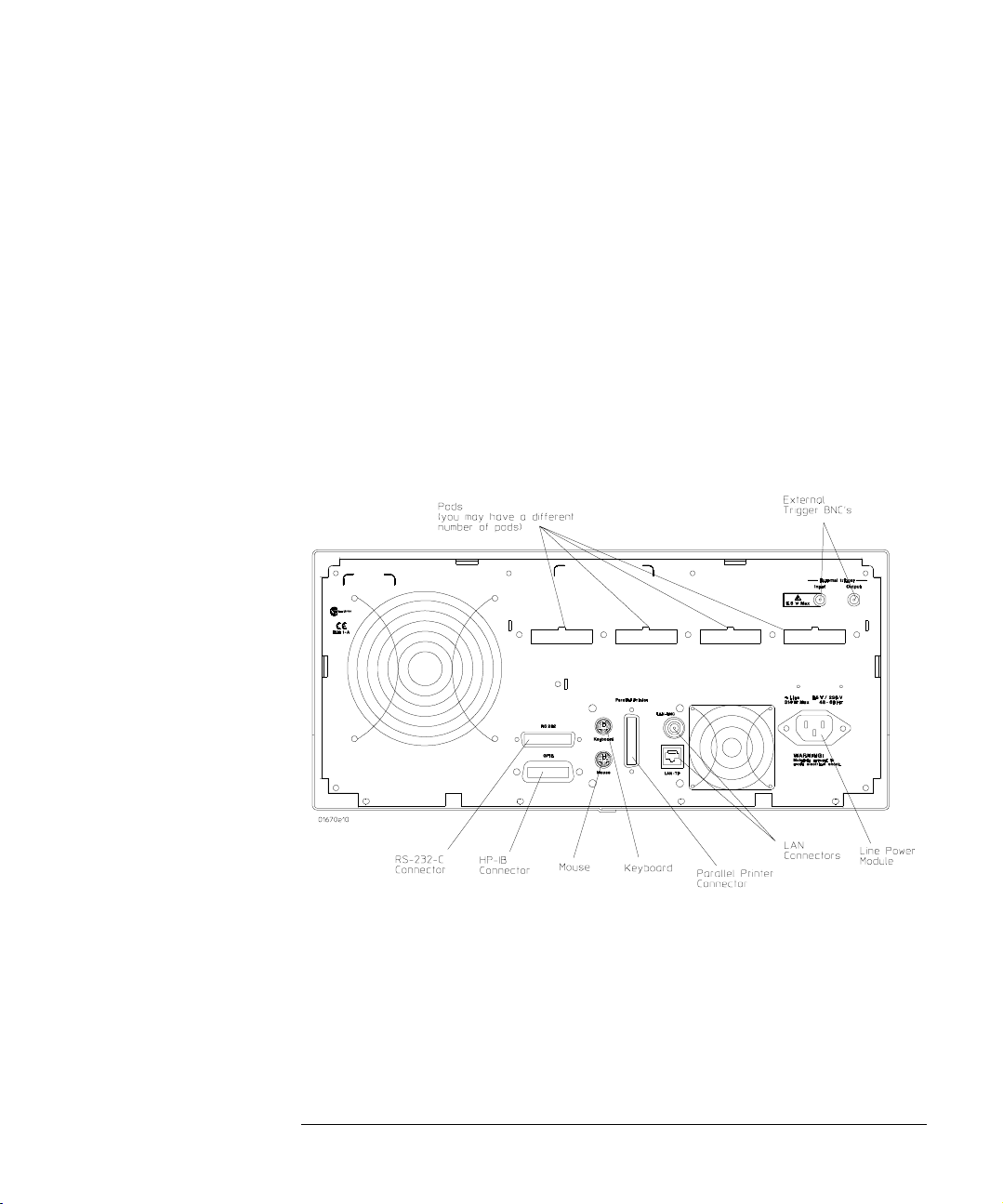
1670G-Series Logic Analyzer Back Panel

Logic Analyzer Overview

Agilent Technologies 1670G-Series Logic Analyzer

External Trigger BNCs

The External Trigger BNCs provide the "Port In" and "Port Out" connections for the Arm In and Arm Out of the Trigger Arming Control menu.

RS-232-C Connector

Standard DB-25 type connector for connecting an RS-232-C printer or controller.

GPIB Connector

Standard GPIB connector for connecting an GPIB printer or controller.

Parallel Printer Connector

Standard Centronics connector for connecting a parallel printer.

LAN Connectors

Connects the logic analyzer to your local ethernet network. The BNC connector on top accepts 10Base2 ("thinlan"). The UTP connector below the BNC connector accepts 10Base-T ("ethertwist").

Calibration Memory Switch

Provides write protection for the calibration factors stored in memory.

Active Probe Power

Provides the power needed for active probes such as the Agilent Technologies 1144A.

Logic Analyzer Overview

Agilent Technologies 1670G-Series Logic Analyzer

To make a measurement

For more detail on any of the information below, see the referenced chapters or the Logic Analyzer Training Kit. If you are using an analysis probe with the logic analyzer, some of these steps may not apply.

Map to target

Connect probes

Connect probes from the target system to the logic analyzer to physically map the target system to the channels in the logic analyzer. Attach probes to a pod in a way that keeps logically-related channels together. Remember to ground the pod.

See Also "Probing" on page 248 for more detail on constructing probes.

Set type

When the logic analyzer is turned on, Analyzer 1 is named Machine 1 and is configured as a timing analyzer, and Analyzer 2 is off. To use state analysis or software profiling, you must set the type of the analyzer in the Analyzer Configuration menu. You can only use one timing analyzer at a time.

Logic Analyzer Overview

Agilent Technologies 1670G-Series Logic Analyzer

Assign pods

In the Analyzer Configuration menu, assign the connected pods to the analyzer you want to use. The number of pods on your logic analyzer depends on the model. Pods are paired and always assigned as a pair to a particular analyzer.

Set up analyzers

Set modes and clocks

Set the state and timing analyzers using the Analyzer Format menu. In general, these modes trade channel count for speed or storage. The state analyzer also provides for complicated clocking. If your state clock is set incorrectly, the data gathered by the logic analyzer might indicate an error where none exists.

See Also "The Analyzer Format Menu" on page 297 for more information on

modes and clocks.

Group bits under labels

The Analyzer Format menu indicates active pod bits. You can create groups of bits across pods or subgroups within pods and name the groups or subgroups using labels.

Logic Analyzer Overview

Agilent Technologies 1670G-Series Logic Analyzer

Set up trigger

Define terms

In the Analyzer Trigger menu, define trigger variables called terms to match specific conditions in your target system. Terms can match patterns, ranges, or edges across multiple labels.

Configure Arming Control

Use Arming Control if:

• you want to correlate the triggers and data of both analyzers

• you want to use the logic analyzer to trigger an external instrument, or

• you want to use an external instrument to trigger the logic analyzer.

Set up trigger sequence

Create a sequence of steps that control when the logic analyzer starts and stops storing data and filters which data it will store. For common tasks, you can use a trigger function to simplify the process or use the user-defined trigger functions to loop and jump in sequence.

See Also "Using the Trigger Menu" on page 70 and "Triggering Examples" on

page 96 for more information on setting up a trigger.

"The Trigger Sequence" on page 391 for more information about the trigger sequence mechanism.

"To save a configuration" on page 136 and "To load a configuration" on page 137 for instructions on saving and loading the setup so you don't have to repeat setting up the analyzer and trigger.

Logic Analyzer Overview

Agilent Technologies 1670G-Series Logic Analyzer

Run measurement

Select single or repetitive

From any Analyzer menu, select the field labeled Run in the upper right corner to start measuring, or press the Run key. A single run will run once, until memory is full; a repetitive run will go until you select Stop or until a stop measurement condition that you set in the markers menu is fulfilled.

If nothing happens, see Troubleshooting the Logic Analyzer

When you start a run, your analyzer menu changes to one of the display menus or a status message pops up. If nothing happens, press the Stop key or select Cancel. If the analyzer still does not display any measurements, see "Troubleshooting the Logic Analyzer" on page 422.

Gather data

You can gather statistics automatically by going to the Waveform or Listing menu, turning on markers, and setting patterns for the X and O markers. You can set the analyzer to stop if certain conditions are exceeded, or just use the markers to count valid runs.

Logic Analyzer Overview

Agilent Technologies 1670G-Series Logic Analyzer

View data

Search for patterns

In both the Waveform and Listing menus you can use symbols and markers to search for patterns in your data. In the Analyzer Waveform or Analyzer Listing menu, toggle the Markers field to turn the pattern markers on and then specify the pattern. When you switch views, the markers keep their settings.

Correlate data

You can correlate data by setting Count Time in your state analyzer's Trigger menu and then using interleaving and mixed display. Interleaving correlates the listings of two state analyzers. Mixed display correlates a timing analyzer waveform and a state analyzer listing. The System Performance Analysis (SPA) Software does not save a record of actual activity, so it cannot be correlated with either timing or state mode.

Logic Analyzer Overview

Agilent Technologies 1670G-Series Logic Analyzer

Make measurements

The markers can count occurrences of events, measure durations, and collect statistics, and SPA provides high-level summaries to help you identify bottlenecks. To use the markers, select the appropriate marker type in the display menu and specify the data patterns for the marker. To use SPA, go to the SPA menu, select the most appropriate mode, fill in the parameters, and press Run.

See Also "System Performance Analysis (SPA) Software" on page 350 for more

information on using SPA.

"The Waveform Menu" on page 334 and "The Listing Menu" on page 332 for additional information on the menu features.

Connecting Peripherals

The 1670G-series logic analyzers comes with a PS2 mouse. It also provides connectors for a keyboard, Centronics (parallel) printer, and GPIB and RS-232-C devices. This chapter tells you how to connect peripheral equipment such as the mouse or a printer to the logic analyzer.

Mouse and Keyboard

You can use either the supplied mouse and optional keyboard, or another PS2 mouse and keyboard with standard DIN connector. The DIN connector is the type commonly used by personal computer accessories.

Printers

The logic analyzer communicates directly with HP PCL printers supporting the printer control language or with other printers supporting the Epson standard command set. Many non-Epson printers have an Epson-emulation mode. HP PCL printers include the following:

• HP ThinkJet

•HP LaserJet

• HP PaintJet

•HP DeskJet

•HP QuietJet

You can connect your printer to the logic analyzer using GPIB, RS-232C, or the parallel printer port. The logic analyzer can only print to printers directly connected to it. It cannot print to a networked printer.

Connecting Peripherals

To connect a mouse

Agilent Technologies supplies a mouse with the logic analyzer. If you prefer a different style of mouse you can use any PS2 mouse with a standard PS2 DIN interface.

1 Plug the mouse into the mouse connector on the back panel.

Make sure the plug shows the arrow on top.

2 To verify connection, check the System External I/O menu for a

mouse box.

The mouse box is on the right side above the Settings fields. If the logic analyzer was displaying the System External I/O menu when you plugged in the mouse, the menu won't update until you exit and then return to it.

The mouse pointer looks like a plus sign (+). To select a field, move the pointer over it and press the left button. To duplicate the front-panel knob, hold down the right button while moving the mouse. Moving the mouse up or to the right duplicates turning the knob clockwise. Moving the mouse down or to the left duplicates turning the knob counterclockwise.

System External I/O Menu Showing Mouse Installed

Connecting Peripherals

To connect a keyboard

You can use either the Agilent-recommended keyboard, E2427B, or any other keyboard with a standard DIN connector.

1 Plug the keyboard into the keyboard connector on the back

panel.

2 To verify, check the System External I/O menu for a keyboard

box.

The keyboard box is on the right side, above the Settings fields. If the logic analyzer was displaying the System External I/O menu while you plugged the keyboard in, the menu won't update until you exit and then return to it.

The keyboard cursor is the location on the screen highlighted in inverse video. To move the cursor, use the arrow keys. Pressing Enter selects the highlighted field. The primary keyboard keys act like the analyzer's front-panel data entry keys.

See Also "Keyboard Shortcuts" on page 267 for complete key mappings.

System External I/O Menu Showing Keyboard Installed

Connecting Peripherals

To connect to an GPIB printer

Printers connected to the logic analyzer over GPIB must support GPIB and Listen Always. When controlling a printer, the analyzer's GPIB port does not respond to service requests (SRQ), so the SRQ enable setting does not have any effect on printer operation.

1 Turn off the analyzer and the printer, and connect an GPIB cable

from the printer to the GPIB connector on the analyzer rear panel.

2 Turn on the analyzer and printer. 3 Make sure the printer is set to Listen Always or Listen Only.

For example, the figure below shows the GPIB configuration switches for an GPIB ThinkJet printer. For the Listen Always mode, move the second switch from the left to the 1 position. Because the instrument doesn't respond to SRQ EN (Service Request Enable), the position of the first switch doesn't matter.

Listen AlwaysSwitchSetting

Connecting Peripherals

4 Go to the System External I/O menu and configure the analyzer's

printer settings. a If the analyzer is not already set to GPIB, select the field under

Connected To: in the Printer box and choose GPIB from the menu.

b Select the Printer Settings field. c In the top field of the pop-up, select the type of printer you

are using. If you are using an Epson graphics printer or an Epson-compatible printer, select Alternate.

d If the default print width and page length are not what you

want, select the fields to toggle them. If you select 132 characters per line when using a printer other than QuietJet, the listings are printed in a compressed mode. QuietJet printers can print 132 characters per line without going to compressed mode, but require wider paper.

e Press Done.

Connecting Peripherals

To connect to an RS-232-C printer

1 Turn off the analyzer and the printer, and connect a null-modem

RS-232-C cable from the printer to the RS-232-C connector on the analyzer rear panel.

2 Before turning on the printer, locate the mode configuration

switches on the printer and set them as follows:

• For the HP QuietJet series printers, there are two banks of mode

function switches inside the front cover. Push all the switches down to the 0 position.

• For the HP ThinkJet printer, the mode switches are on the rear panel of

the printer. Push all the switches down to the 0 position.

• For the HP LaserJet printer, the factory default switch settings are

okay.

3 Turn on the analyzer and printer. 4 Go to the System External I/O menu and configure the analyzer's

printer settings. a If the analyzer is not already set to RS232, select the field

under Connected To: in the Printer box and choose RS232 from the menu.

b Select the Printer Settings field. c In the top field of the pop-up, select the type of printer you

are using. If you are using an Epson graphics printer or an Epson-compatible printer, select Alternate.

Connecting Peripherals

d If the default print width and page length are not what you

e Press Done.

5 Select the RS232 Settings field and check that the current

settings are compatible with your printer.

See Also "The RS-232-C, GPIB, and Centronics Interface" on page 282 for more

information on RS-232-C settings.

Connecting Peripherals

To connect to a parallel printer

1 Turn off the analyzer and the printer, and connect a parallel

printer cable from the printer to the parallel printer connector on the analyzer rear panel.

2 Before turning on the printer, configure the printer for parallel

operation.

The printer's documentation will tell you what switches or menus need to be configured.

3 Turn on the analyzer and printer. 4 Go to the System External I/O menu and configure the analyzer's

printer settings. a If the analyzer is not already set to Parallel, select the field

under Connected To: in the Printer box and choose Parallel from the menu.

b Select the Printer Settings field. c In the top field of the pop-up, select the type of printer you

are using. If you are using an Epson graphics printer or an Epson-compatible printer, select Alternate.

d If the default print width and page length are not what you

e Press Done.

There are no settings specific to the parallel printer connector.

Connecting Peripherals

To connect to a controller

You can control the 1670G-series logic analyzer with another instrument, such as a computer running a program with embedded analyzer commands. The steps below outline the general procedure for connecting to a controller using GPIB or RS-232-C.

1 Turn off both instruments, and connect the cable.

If you are using RS-232-C, the cable must be a null-modem cable. If you do not have a null-modem cable, you can purchase an adapter at any electronics supply store.

2 Turn on the logic analyzer and then the controller. 3 In the System External I/O menu, select the field under

Connected To: in the Controller box and set it appropriately.

4 Select the appropriate Settings field and configure the values in

the pop-up menu to be compatible with the controller.

See Also Agilent Technologies 1670G-Series Logic Analyzers Programmer's

Guide and the LAN section of this book starting on page 476 for more information on connecting controllers.

Using the Logic Analyzer

This chapter shows you how to perform the basic tasks necessary to make a measurement. Each section uses an example to show how the task fits into the overall goal of making a measurement.

Using the Logic Analyzer

Accessing the Menus

When you power up the logic analyzer, the first screen after the system tests is the Analyzer Configuration menu. Menus are identified by two fields in the upper left corner. The leftmost field shows Analyzer. This field is sometimes referred to as the "mode field" because it controls which other set of menus you can access. The second field, just to the right of the mode field, accesses menus within the mode and so is called the "menu field." For example, if you are in Analyzer mode, the menus for the analyzer are accessed from the menu field. Menus are referred to by the titles that appear in the mode and menu fields, for example, the Analyzer Configuration menu.

The figure below shows the top of the first screen. The mode field, item 1, displays "Analyzer." The menu field, item 2, displays "Configuration." Because menus are identified by the titles in these two fields, this menu is referred to as the Analyzer Configuration menu. When there is no risk of confusion, the menu is sometimes referred to just by the title showing in the second field, for example, the Configuration menu.

Using the Logic Analyzer

Accessing the Menus

To access the System menus

The System menus allow you to perform operations that affect the entire logic analyzer, such as load configurations, change colors, and perform system diagnostics.

1 Select the mode field.

Use the arrow keys to highlight the mode field, then press the Select key. Or, if you are using the mouse, click on the field. This operation is referred to as "select."

A pop-up menu appears with the choices System and Analyzer. (If you have installed any optional software, there may be other choices as well.)

2 Select System.

Using the Logic Analyzer

Accessing the Menus

3 Select the menu field.

The pop-up lists five menus: Hard Disk, Flexible Disk, External I/O, Utilities, and Test.

• Hard Disk allows you to perform file operations on the hard disk.

To access the Analyzer menus

The Analyzer menus allow you to control the analyzer to make your measurement, perform operations on the data, and view the results on the display.

1 Select the mode field.

A pop-up menu appears with the choices System, Analyzer, and Patt Gen or Scope (if you have one of these options). If you have installed any optional software, there may be other choices as well.

2 Select Analyzer. 3 Select the menu field.

The figure on the next page does not show all of the possible menus because certain menus are only accessible with the analyzer configured in a particular mode. For instance, the Compare menu is only available when you set an analyzer to state mode, and the SPA menu requires an analyzer set to SPA.

• Configuration is always available in Analyzer mode. Use Configuration to assign pods and set the analyzer type.

• Format is available whenever an analyzer is set to a type other than "Off." Use Format to create data labels and symbols, adjust the pod threshold level, and set modes and clocks.

• Trigger is available when an analyzer is set to State or Timing. Use Trigger to specify a trigger sequence which will filter the raw information into the measurement you want to see.

• Listing is available when an analyzer is set to State or Timing. Use Listing to view your measurement as a list of states. Using an inverse assembler, a state analyzer can display the measurement as though it were assembly code.

Using the Logic Analyzer

Accessing the Menus

• Compare is available only when an analyzer is set to State. Use Compare to compare two listings and quickly scroll to the sections where they differ.

• Mixed Display always appears in the menu list when an analyzer is set to State or Timing, but it requires a State analyzer with time tags enabled.

• Waveform is available when an analyzer is set to State or Timing. Use Waveform to view the data as logic levels on discrete lines.

Using the Analyzer Menus

The following examples show how to use some of the Analyzer menus to configure the logic analyzer for measurements. These examples assume that you have already determined which signals are of interest, and have connected the logic analyzer to the target system. Some of the examples use data from a Motorola 68360 target system, acquired with an Agilent Technologies E2456A Analysis Probe.

To label channel groups

Agilent Technologies logic analyzers give you the ability to separate or group data channels and label the groups with a name that is meaningful to your measurement. Labels also assist you in triggering only on states of interest.

Labels can only be assigned in the Analyzer Format menu. Once assigned, the labels are available in all display menus, where they can be added to or deleted from the display. Use labels when you want to group data channels by function with a name that has meaning to that function.

The default label names are Bus1 through Bus126. However, you can modify a name to any six-character string. If you are using an Agilent Technologies analysis probe, the configuration file has predefined labels for your specific processor.

Using the Logic Analyzer

Using the Analyzer Menus

To create or modify a label and assign channel groups, use the following procedure.

1 Press the Format key to go to the Format menu. 2 Select a label under the Labels heading. In the pop-up menu,

select Modify Label.

3 Use the front panel to enter a name for the label and press Done.

In this example, the label is called CYCLE.

4 Select the pod containing the channels for the label. Use the

knob or the arrow keys to position the selector over a channel you want to change.

An asterisk indicates the channel is selected; a dot indicates the channel is not part of the current group.

Using the Logic Analyzer

Using the Analyzer Menus

5 Toggle the channel's group status by pressing Select.

The indicator changes and the selector moves to the next channel.

6 Press the Done key to complete selection.

Using the Logic Analyzer

Using the Analyzer Menus

To create a symbol

Symbols are alphanumeric mnemonics that represent specific data patterns or ranges. When you define a symbol and set the base type to Symbol in the Listing menu, the symbol is displayed in the data listing where the bit pattern would normally be displayed. The symbols also appear in the Waveform menu when you view a label in bus form. Symbols allow you to quickly identify data of interest.

To create a symbol, use the following procedure.

1 In the Analyzer Format menu, select Symbols.

The symbol table menu appears. The symbol table is where all user symbols are created and maintained. If you get a message, "No labels specified," check that you have at least one label turned on with channels assigned to it.

2 In the Symbol menu, select the Label field. In the pop-up menu,

select the label that contains the channel groups you want.

When you open the symbol table menu, the Label field displays the name of the first active label.

If the label you want does not appear in the pop-up menu, the label is probably off. Return to the Format menu, select the label you want, and select Turn Label On. Another possibility is that the label is on the other analyzer. The two analyzers manage resources separately.

3 Select the Base field. In the pop-up menu, select the base for the

pattern.

In this example, binary is used because CYCLE only contains three channels.

4 Select the field below Symbol. Select Add a Symbol, type in the

symbol name, then press Done.

Using the Logic Analyzer

Using the Analyzer Menus

5 If additional Symbols are needed, repeat step 4 until you have

added all symbols.

In this example, three symbols are added: MEM RD, MEM WR, and DATA RD.

6 Toggle the Type field to "range" or "pattern".

When Type is range, a third field appears under the Stop column. To fully specify a range, you need to enter a value for it, too.

7 Select the Pattern/Start field and use the keypad to enter an

appropriate value in the selected base. Use X for "don't care."

8 When the pattern is specified, press Done. If you created

additional Symbols, repeat steps 6 and 7 until all symbols are specified.

9 To close the symbol table menu, select Done.

Symbol table Menu Showing Three Symbols

You can also download symbol tables created by your programming environment using the Symbol Utility. The Symbol Utility is shipped installed on all 1670G-series logic analyzers.

See Also The Symbol Utility section of this book on page 563 for more

information on the Symbol Utility.

Using the Logic Analyzer

Using the Analyzer Menus

To examine an analyzer waveform

The Analyzer Waveform menu lets you view state or timing data in a format similar to an oscilloscope display. The horizontal axis represents states (in state mode) or time (in timing mode) and the vertical axis represents logic highs and lows.

1 In Analyzer mode, press the Run key to acquire data.

In any mode other than Analyzer, Scope, or Patt Gen, pressing the Run key has no effect. The menus which ignore Run, lack the Run field onscreen. In Analyzer mode with Run available, the menu changes to a display menu.

2 Go to the Analyzer Waveform menu. 3 To adjust the horizontal axis (sec/Div or states/Div), use the

knob.

If nothing happens when you turn the knob, make sure the Div field has a roll indicator above it, as in the figures on the next page. When you first enter the Waveform menu, the knob adjusts the horizontal axis but if you select another rollable field, the knob will control that field instead.

4 To adjust the display relative to the trigger, select the Delay field

and enter a value or use the knob.

The portion of memory being displayed is indicated by a white bar along the bottom of the display area. The position of the trigger in memory is indicated by a red dot on the same line. When the bar includes the dot, then the trigger is visible on the display as indicated by a vertical line with a "t" underneath.

Using the Logic Analyzer

Using the Analyzer Menus

5 To scroll through waveforms, select the large rectangle below the

Div field and use the knob.

The roll indicator appears at the top of the rectangle and the name of the first waveform is highlighted. The highlight moves as you turn the knob.

6 To insert waveforms, double-click on the large rectangle under

the Div field (sec/Div or states/Div). In the pop-up, select Insert, and then select the labels and channels.

The Sequential field inserts all the channels of the label as individual waveforms; the Bus field groups the waveforms; the Bit N field inserts just the Nth bit. Waveforms are inserted after the currently highlighted one.

7 To take measurements, select the Markers field and choose the

appropriate marker type.

The markers available depend on the type of analyzer and whether or not tagging is enabled. Use markers to locate patterns quickly.

Using the Logic Analyzer

Using the Analyzer Menus

Example The following example shows a state waveform from the Agilent

Technologies analysis probe for the Motorola 68360. Notice how the bus waveforms insert symbols or state data.

Using the Logic Analyzer

Using the Analyzer Menus

To examine an analyzer listing

The Analyzer Listing menu displays state or timing data as patterns (states). The Listing menu uses any of several formats to display the data such as binary, ASCII, or symbols. If you are using an inverse assembler and select Invasm, the data is displayed in mnemonics that closely resemble the microprocessor source code.

See Also "The Inverse Assembler" at the end of this chapter for additional

information on using an inverse assembler.

1 In Analyzer mode, press the Run key to acquire data.

In any mode other than Analyzer, Scope, or Patt Gen, pressing the Run key has no effect. The menus which ignore Run lack the Run field onscreen. In Analyzer mode with Run available, the menu changes to a display menu.

2 Go to the Analyzer Listing menu.

All labels defined in the Analyzer Format menu appear in the listing. If there are more labels than will fit on the screen, the Label/Base field is shaded like a normal field.

3 To scroll the labels, select the Label/Base field and use the knob

or press the blue shift key and a page key.

If the Label/Base field is selectable, the roll indicator appears over the field as in the example. To move the labels one full screen at a time, press Shift and a Page key.

Using the Logic Analyzer

Using the Analyzer Menus

4 To scroll the data, use the Page keys or select the data roll field

and use the knob.

If you select the data roll field, the roll indicator moves to it. No matter which field is currently controlled by the knob, however, the Page keys page the data up or down.

The numbers in the data roll column indicate how many samples the data is from the trigger. Negative numbers occurred before the trigger and positive numbers occurred after.

5 If the labels have symbols associated with them, set the base to

Symbol.

The symbols you defined appear in the listing.

6 To insert a label, select one of the label fields, then select Insert

from the pop-up and the label you want to insert.

The last label cannot be deleted, so there is always at least one label. You can insert the same label multiple times and display it in different bases.

7 To take measurements, select the Markers field and choose the

appropriate marker type.

The markers available depend on the type of analyzer and whether or not tagging is enabled. Use markers to locate states quickly.

Using the Logic Analyzer

Using the Analyzer Menus

Example The following illustration shows a listing from the Agilent Technologies

analysis probe for the Motorola 68360. The ADDR label has the base set to Hex to conserve space on the display. The DATA label has the base set to Invasm for inverse assembly. The FC label has the base set to Symbol. Additional labels are located to the right of FC, and can be viewed by highlighting and selecting Label, then using the knob to scroll the display horizontally.

Using the Logic Analyzer

Using the Analyzer Menus

To compare two listings

The Compare menu allows you to take two state analyzer acquisitions and compare them to find the differences. You can use this function to quickly find all the effects after changing the target system or to quickly compare the results of quality tests with results from a working system.

1 In Analyzer mode, press the Run key to acquire data.

2 Go to the Analyzer Compare menu, select Copy Listing to

Reference, and then select Execute.

The Compare menu initially is empty, but when you select Execute the data appears.

3 Set up the other test that you want to compare to the first.

This can be a change to the hardware, or a different system. Do not change the trigger, however, or all the states will be different.

4 Run the test again, then select the Reference listing field to

toggle to Difference listing.

The Difference listing is displayed on the next page.

Using the Logic Analyzer

Using the Analyzer Menus

The Difference listing displays the states that are identical in dark typeface, and the states that are different in light typeface (indistinguishable in the above illustration). The light typeface shows the data from the compare file that is different from the data in the reference file.

5 Select the Find Error field and use the knob to scroll through

the errors.

The display jumps past all states that are identical, and shows the number of errors through the current state in the Find Error field. In the above illustration, there are 37 errors through state 44 of the listing.

Using the Logic Analyzer

The Inverse Assembler

When the analyzer captures a trace, it captures binary information. The analyzer can then present this information in symbol, binary, octal, decimal, hexadecimal, or ASCII. Or, if given information about the meaning of the data captured, the analyzer can inverse assemble the trace. The inverse assembler makes the trace list more readable by presenting the trace results in terms of processor opcodes and data transactions.

To use an inverse assembler

Most analysis probes include an inverse assembler in their software. Loading the configuration file for the analysis probe sets up the logic analyzer to provide certain types of information for the inverse assembler. This section is provided in case you ever have to set up an analyzer for inverse assembly yourself.

The inverse assembly software needs at least these five pieces of information:

• Address bus. The inverse assembler expects to see the label ADDR, with bits ordered in a particular sequence.

• Data bus. The inverse assembler expects to see the label DATA, with bits ordered in a particular sequence.

• Status. The inverse assembler expects to see the label STAT, with bits ordered in a particular sequence.

• Start state for disassembly. This is the first displayed state in the trace list, not the cursor position. See the figure on the next page.

• Tables indicating the meaning of particular status and data combinations.

Using the Logic Analyzer

The Inverse Assembler

The particular sequences that each label requires depends on the type of chip the inverse assembler was designed for. Because of this, inverse assemblers cannot generally be transferred between platforms.

To run the inverse assembler, you must be sure the labels are spelled correctly as shown here, or as directed in your inverse assembler documentation. Even a minor difference such as not capitalizing each letter will cause the inverse assembler to not work.

Inverse Assembly Synchronization

When you press the Invasm key to begin inverse assembly of a trace, the inverse assembler begins with the first displayed state in the trace list. This is called synchronization. It looks at the status bits (STAT) and determines the type of processor operation, which is then displayed under the STAT label. If the operation is an opcode fetch, the inverse assembler uses the information on the data bus to look up the corresponding opcode in a table, which is displayed under the DATA label. If the operation is a data transfer, the data and corresponding operation are displayed under the DATA label. This continues for all subsequent states in the trace list.

Using the Logic Analyzer

The Inverse Assembler

If you roll the trace list to a new position and press Invasm again, the inverse assembler repeats the above process. However, it does not work backward in the trace list from the starting position. This may cause differences in the trace list above and below the point where you synchronized inverse assembly. The best way to ensure correct inverse assembly is to synchronize using the first state you know to be the first byte of an opcode fetch.

See Also The Analysis Probe User's Guide for more information on controlling

inverse assembly. If you have problems using the inverse assembler, see "Troubleshooting the Logic Analyzer" on page 421.

Using the Logic Analyzer

The Inverse Assembler

Using the Trigger Menu

To use the logic analyzer efficiently, you need to be able to set up your own triggers. This chapter provides examples of triggering. Those examples assume you already know where to find fields in the trigger menu.

This chapter shows you how to:

• Specify a basic trigger

• Change a trigger sequence

• Set up time correlation between analyzers

• Arm from another instrument, or arm another instrument

• Manage memory

Using the Trigger Menu

Specifying a Basic Trigger

The default analyzer triggers are

While storing "anystate" TRIGGER on "a" occuring 1 time Store "anystate"

for state analyzers and

TRIGGER on "a" > 8 ns

for timing analyzers. If you want to simply record data, these will get you started. They can quickly be tailored by specifying a particular pattern to look for instead of the general case.

Customizing a trigger generally requires these steps:

•Assign terms.

• Define the terms.

• Change the trigger to use the new terms.

Using the Trigger Menu

Specifying a Basic Trigger

To assign terms to an analyzer

When you turn the logic analyzer on, Analyzer 1 is named Machine 1 and Analyzer 2 is off. Because trigger terms can only be used by one analyzer at a time, all the terms are assigned to Analyzer 1. If you plan to use both analyzers in your measurement, you need to assign some of the terms to Analyzer 2.

1 Go to the Trigger Machine 1 menu.

If you have renamed Machine 1 in the Analyzer Configuration menu, the name you changed it to will appear in the menu instead of Machine

2 Select a term.

The terms are the fields below the roll field "Terms". See the figure below.

3 Select Assign from the list that appears.

The Resource Term Assignment menu appears. It is divided into two sections, one for each analyzer. All terms are listed.

Using the Trigger Menu

Specifying a Basic Trigger

4 To change a term assignment, select the term field.

The term fields toggle from one section to the other. You can get all your terms assigned at once, or just change a few to meet immediate needs.

5 To exit the term assignment menu, select Done.

Using the Trigger Menu

Specifying a Basic Trigger

To define a term

Both default triggers trigger on term "a". If you only need to look for the occurrence of a certain state, such as a write to protected memory, then you only need to define term "a" to make the measurement you want.

1 In the Trigger menu, select the field at the intersection of the

term and the label whose value you want to trigger on.

You set labels in the Analyzer Format menu. If the channels you want to monitor are not attached to a label, they will not appear in the trigger menu.

2 Enter the value or pattern you want to trigger on.

If the label's base is Symbol, a pop-up menu appears offering a choice of symbols. For other bases, use the keypad. An "X" stands for "don't care".

If there are two conditions that need to be present at the same time, for example a protected address on the address bus and a write on the read/write line, define both values on the same term. See the figure below.

3 Press Done.

Term "a" Defined as a Data Write to Read-Only Memory

Using the Trigger Menu

Specifying a Basic Trigger

To change the trigger specification

Most triggers use terms other than "a." Even a simple trigger might use additional terms to set conditions on the actual trigger. To use these terms, you must include them in the trigger sequence specification.

1 In the Trigger menu, select the number beside the specific level

you want to modify.

A Sequence Level menu pops up. It shows the current specification for that trigger level.

2 Select the field you want to change.

In the top row of the pop-up are three action fields: Insert Level, Select New Function, and Delete Level. The next section goes into detail on them. The fields after "While storing", "TRIGGER on", and "Else on" are completed with trigger terms. Selecting these fields pops up a menu of terms.

3 Select the term you want to use from the pop-up, or enter a new

value, as appropriate to the field.

If you have renamed a term, that name is automatically used everywhere the term would appear.

Using the Trigger Menu

Specifying a Basic Trigger

4 Select Done until you are back at the Trigger menu.

Term Selection Pop-up Menu

Using the Trigger Menu

Changing the Trigger Sequence

Most measurements require more complicated triggers to better filter information. From the basic trigger, you can:

• Add sequence levels

• Change trigger functions

Your logic analyzer provides a trigger function library to make setting up the trigger easier. There are 12 state functions and 13 timing functions. Most trigger functions take more than one level internally to implement, and can be broken down into their separate levels. Once broken down, the levels can be used to design your own trigger sequences.

Using the Trigger Menu

Changing the Trigger Sequence

To add sequence levels

You can add sequence levels anywhere except after the final one.

1 In the Trigger menu, select the number beside the sequence level

just after where you want to insert.

For example, if you want to insert a sequence level between levels 1 and 2, you would select level 2. To insert levels at the beginning, select level 1.

A Sequence Level pop-up appears. Its exact contents depend on the analyzer configuration and the level specification. However, all Sequence Level pop-ups have an Insert Level field in the upper left corner.

2 Select Insert Level.

Another pop-up offers the choices of Cancel, Before, or After. If the level you started from was the last level, After will not appear.

3 Select Before.

The Trigger Function pop-up replaces the Sequence Level pop-up. The functions available depend on whether the analyzer is configured as state or timing.

4 Use the knob to highlight a trigger function, and select Done.

A new Sequence level pop-up appears. Its contents reflect the trigger function you just selected. The figure below shows a user trigger function for a state analyzer.

5 Fill in the fields and select Done.

Sequence Level Pop-up Menu

Using the Trigger Menu

Changing the Trigger Sequence

Using the Trigger Menu

Changing the Trigger Sequence

To change trigger functions

You do not need to add and delete levels just to change a level's trigger function. This can be done from within the Sequence Level pop-up.

1 From the Trigger menu, select the sequence level number of the

sequence level you want to modify.

A Sequence Level pop-up appears. Its contents reflect the current trigger function.

2 Select Select New Function.

The Trigger Function pop-up replaces the Sequence Level pop-up. The functions available depend on whether the analyzer is configured as state or timing.

3 Use the knob to highlight the function you want, and select

Done.

A new Sequence Level pop-up appears. Its contents reflect the function you just selected. The wording of this screen is very similar to the function description, and the line drawing demonstrates what the function is measuring.

4 Select the appropriate assignment fields and insert the desired

pre-defined terms, numeric values, and other parameter fields required by the function. Select Done.

For state analyzers, a final "go to trigger" level is automatically placed at the end of the trigger specification for you. This level must always be a user level. Although you can change its fields, you cannot change the function. Timing analyzers do not have this restriction.

See Also "Timing Trigger Function Library" and "State Trigger Function Library"

in The Analyzer Trigger Menu on page 312 for a complete listing of functions.

Using the Trigger Menu

Setting Up Time Correlation between Analyzers

There are two possible combinations of analyzers: state and state, and state and timing. Timing and timing is not possible because the Analyzer Configuration menu only permits one analyzer at a time to be configured as a timing analyzer. For either combination, time correlation is necessary for interleaving and mixed display.

Time correlation is useful when you want to store different sorts of data for each trace, but see how they are related. For instance, you could set up a timing and a correlated state analyzer and see if setup and hold times are being met. Or, you could set up two state analyzers and have one watch normal program execution and the other watch the control and status lines.

Time correlation requires that state analyzers store time tags. You set the state analyzer to store time tags by turning on Count Time in the Analyzer Trigger menu. The timing analyzer already stores time tags when it samples data.

See Also "Special displays" on page 128 for more information on interleaving and

mixed display.

Using the Trigger Menu

Setting Up Time Correlation between Analyzers

To set up time correlation between two state analyzers

To correlate the data between two state analyzers, both must have Count Time turned on in their Trigger menus. Although both have Count State available, it is not possible to correlate data based on states even when they are identically defined.

1 In the Analyzer Trigger menu, select Count.

Count may be Count Off, Count Time, or Count States. Selecting the field causes a pop-up to appear.

2 Select the field after Count: and select Time.

A warning may appear about reduced memory. It will not prevent you from changing Count to Count Time.

3 Select Done. 4 Repeat steps 1 through 3 for the other state analyzer.

Now when you acquire data you will be able to interleave the listings.

Using the Trigger Menu

Setting Up Time Correlation between Analyzers

To set up time correlation between a timing and a state analyzer

To set up time correlation between a timing and a state analyzer, only the state analyzer needs to have Count Time turned on. The timing analyzer automatically keeps track of time.

1 In the state Analyzer Trigger menu, select Count.

Count may be Count Off, Count Time, or Count States. Selecting the field causes a pop-up to appear.

2 Select the field after Count: and select Time.

A warning may appear about reduced memory. It will not prevent you from changing Count to Count Time.

3 Select Done.

Now when you acquire data you will be able to set up a mixed display.

Using the Trigger Menu

Arming and Additional Instruments

Occasionally you may need to start the analyzer acquiring data when another instrument detects a problem. Or, you may want to have the analyzer itself arm another measuring tool. This is accomplished from the Arming Control field of the Analyzer Trigger menu.

To arm another instrument

1 Attach a BNC cable from the External Trigger Output port on the

back of the logic analyzer to the instrument you want to trigger.

The External Trigger Output port is also referred to as "Port Out." It uses standard TTL logic signal levels, and will generate a rising edge when trigger conditions are met.

2 In the Analyzer Trigger menu, select Arming Control.

Arming Control is below the Run button.

3 Select the field near Arm Out, and choose PORT OUT. 4 If you are using both analyzers, set the Arm Out Sent From field

in the upper right corner.

This field does not appear if only one analyzer is configured.

The selected analyzer will send the arm signal when it finds its trigger.

5 Select Done.

When you make a measurement, the analyzer will send an arm signal through the External Trigger Output when the analyzer finds its trigger.

Using the Trigger Menu

Arming and Additional Instruments

To arm the oscilloscope with the analyzer (1670G-series logic analyzers with the oscilloscope option)

If both analyzer and the oscilloscope are turned on, you can configure one analyzer to arm the other analyzer and the oscilloscope. An example of this is when a state analyzer triggers on a bit pattern, then arms a timing analyzer and the oscilloscope which capture and display the waveform after they trigger.

1 In the Analyzer Trigger menu, select Arming Control. 2 Select the Analyzer Arm Out Sent From field, and choose from

the list the Analyzer that will generate the arm.

3 Select the Analyzer Arm In field, and choose Group Run.

This allows you to time-correlate the data from the analyzers and the scope. The Scope Trigger Mode must be Immediate for correlation.

4 Select the field of the instrument which will arm the others, and

in the pop-up set it to run from Group Run.

The Scope field is not selectable. To set how the scope is run, select the field under Scope Arm In.

5 Select the other instrument fields and choose the mechanism

which will arm them.

The Analyzer Arm Out field determines which analyzer sends the arming signal to Port Out and to the oscilloscope if the oscilloscope is being armed by an analyzer.

As you set each machine, the arrows connecting the fields in the Arming Control menu change. The arrows show the order in which the instruments are armed.

See the example on the next page.

6 Select Done until you are back at the Trigger menu.

Using the Trigger Menu

Arming and Additional Instruments

Example In this example STATE MACH triggers from Group Run, then arms

TIME MACH and Scope.

To duplicate this, set STATE MACH to run from Group Run, TIME MACH to run from STATE MACH, and Scope Arm In to Analyzer.

Arming with two analyzers and an oscilloscope

When the run starts, the state analyzer automatically begins evaluating its trigger sequence instruction. When the trigger sequence is satisfied, the state analyzer sends an “Arm” signal to the timing analyzer, the oscilloscope, and the external trigger.

Arming and Additional Instruments

To receive an arm signal from another instrument

When you set the analyzer to wait for an arm signal, it does not react to data that would normally trigger it until after it has received the arm signal. The arm signal can be sent to any of the Trigger Sequence levels, but will go to level 1 unless you change it. Setting up the analyzer to receive an arm signal is more efficient when the sequence levels are already in place.

1 Connect a BNC cable from the instrument which will be sending

the signal to the External Trigger Input port on the back of the

CAUTION: Do not exceed 5.5 volts on the External Trigger Input.

logic analyzer.

The External Trigger Input port is also referred to as "Port In." It uses standard TTL logic signal levels, and expects a rising edge as input.

Using the Trigger Menu

2 In the Analyzer Trigger menu, select Arming Control.

Arming Control is below the Run button.

3 Select the leftmost field, and choose PORT IN.

The field is unlabeled and shows either Run or PORT IN. It has arrows going from it to the analyzer(s).

Using the Trigger Menu

Arming and Additional Instruments

4 To change the default settings, select the analyzer field.

A small pop-up menu appears. To change which device the analyzer is receiving its arm signal from, select the Run from field. To change which sequence level is waiting for the arm signal, select the Arm sequence level field.

5 Select Done until you are back at the Trigger menu.

Using the Trigger Menu

Managing Memory

Sometimes you will need every last bit of memory you can get on the logic analyzer. There are three simple ways to maximize memory when specifying your trigger:

• Selectively store branch conditions (state only)

• To set the memory length

• Place the trigger relative to memory

• Set the sampling rates (timing only)

Using the Trigger Menu

Managing Memory

To selectively store branch conditions (state only)

Besides setting up your trigger levels to store anystate, no state, or some subset of states, you can also choose whether or not to store branch conditions. Branch conditions are always stored by default, and can make tracing the analyzer's path through a complicated trigger easier. If you really need the extra memory, however, it is possible to not store the branch conditions.

You cannot set the analyzer to store only some branches in a trigger sequence specification.

1 In the Analyzer Trigger menu, select Acquisition Control.

The Acquisition Control menu pops up. If the acquisition mode is set to Automatic, the menu contains a single field and an explanation. If Acquisition has been customized, it has 3 fields and a picture showing where the trigger is currently placed in memory.

2 If the mode is Automatic, select the field and toggle it to Manual.

The menu now shows three fields and a picture.

3 Select the Branches Taken Stored field.

It toggles to Branches Taken Not Stored.

4 Select Done.

Using the Trigger Menu

Managing Memory

To set the memory length

The 1670G-series logic analyzer’s memory length can be adjusted. The table on the following page shows the amount of memory available for different modes of operation.

Typically you will want to use small amounts of memory at the beginning of troubleshooting, when you are first looking for a problem, and use deep memory when you are searching for the root cause. Shallower memory provides faster acquisitions, but might not have sufficient context. Deep memory provides more context, but takes longer to fill, more time to display, and more time for you to analyze. The Memory Length field allows you to configure the acquisition memory to suit your needs.

1 In the Analyzer Trigger menu, select Acquisition Control.

The Acquisition Control menu pops up. If the acquisition mode is set to Automatic, the menu contains two fields and an explanation. If Acquisition has been customized, it has four or five fields and a picture showing the amount of memory and where the trigger is currently placed in memory.

2 Select the Memory Length field.

Use the knob to select the memory length. Memory size can be set in powers of 2 from 4096 to the maximum. The table below shows the maximum memory for various modes of operation.

Using the Trigger Menu

Managing Memory

3 Select Done to exit the Acquisition Control menu.

Mode Memory Option 001 Option 002

Full-channel timing >64K (65536) 256K 2M

Half-channel timing >128K (131072) 512K 4M

State

State Compare

With tags turned off or non-interleaved tags. Tags are non-interleaved

>64K (65536) 256K 2M

>32K (32768) 128K 1M

>32K (32768) 128K 512K

>32K (32768) 128K 256K

if there is an unassigned pod pair or a pod pair assigned to an analyzer that is turned off.

With interleaved tags.

Using the Trigger Menu

Managing Memory

To place the trigger in memory

In Automatic Acquisition Mode, the exact location of the trigger depends on the trigger specification but usually falls around the center. You can manually place it at the beginning, end, or anywhere else.

1 In the Analyzer Trigger menu, select Acquisition Control.

The Acquisition Control menu pops up. If the acquisition mode is set to Automatic, the menu contains a single field and an explanation. If Acquisition has been customized, it has 3 or 4 fields and a picture showing where the trigger is currently placed in memory.

2 If the mode is Automatic, select the field to toggle it to Manual.

The menu now shows three fields and a picture.

3 Select the Trigger Position field. 4 Select the appropriate entry for your needs.

Start, Center, and End place the trigger respectively at the beginning, middle, and end of the memory. Delay, available in timing analyzers only, causes the analyzer to not save any data before the time delay has elapsed. User Defined calls up a fourth field where you specify exactly where you want the trigger.

5 Select Done.

Using the Trigger Menu

Managing Memory

To set the sampling rates (Timing only)

A timing analyzer samples the data based on its own internal clock. A short sample period provides more detail about the device under test; a long sample period allows more time before memory is full. However, if the sample period is too large, some information may be missed.

1 In the Analyzer Trigger menu, select Acquisition Control.

The Acquisition Control menu pops up. If the acquisition mode is set to Automatic, the menu contains a single field and an explanation. If Acquisition has been customized, it has 3 or 4 fields and a picture showing where the trigger is currently placed in memory.

2 If the mode is Automatic, select the field and toggle it to Manual.

The menu now shows three fields and a picture.

3 Set the Sample Period field using the knob, or select it to use

the keypad to enter the period.

4 Select Done.

Next time you take a measurement, the analyzer will sample at the rate you entered.

Triggering Examples

As you begin to understand a problem in your system, you may realize that certain conditions must occur before the problem occurs. You can use sequential triggering to ensure that those conditions have occurred before the analyzer recognizes its trigger and captures information.

If you are not familiar with the trigger menus, read through Chapter 4, "Using the Trigger Menu," and try working through the examples in the Logic Analyzer Training Kit manual.

Triggering Examples

Single-Machine Trigger Examples

The following examples require only a single analyzer to make measurements. Sequence specifications are given in the form you see within the sequence levels, but the illustrations show the complete, multi-level sequence specification.

Although all the examples are case-specific, terms are named in a way that highlights their role in solving the trigger problem. You can easily apply the examples to your specific instance by changing the specific values assigned to the trigger terms.

Triggering Examples

Single-Machine Trigger Examples

To store and time the execution of a subroutine

Most system software of any kind is composed of a hierarchy of functions and procedures. During integration, testing, and performance evaluation, you want to look at specific procedures to verify that they are executing correctly and that the implementation is efficient. The analyzer lets you do this by triggering on entry to the address range of the subroutine and counting the elapsed time since the trigger state.

1 Go to the state analyzer's Trigger menu. 2 Set Count to Time. 3 Define a range term, such as Range1, to represent the address

range of the particular subroutine.

You may need to examine the structure of your code to help determine this. If your subroutine calls are really procedure calls, then there is likely to be some code at the beginning of the routine that adjusts the stack for local variable allocation. This will precede the address of the first statement in the procedure. If your subroutine has no local storage and is called by a jump or branch, then the first statement will also be the entry address.

4 Under State Sequence Levels, enter the following sequence

specification:

• While storing "no state" TRIGGER on "In_Range1" Occurs 1 Else on "no state" go to level 1

• While storing "In_Range1" Then find "Out_Range1" Occurs 1 Else on "no state" go to level 2

• Store "no state" on "no state" go to level 1

NOTE: For processors that prefetch instructions or have pipelined architectures, you

may want to add part or all of the depth of the pipeline to the start address for In_Range1 to ensure that the analyzer does not trigger on a prefetched but unexecuted state.

Triggering Examples

Single-Machine Trigger Examples

The figure below shows what you would see on your analyzer screen after entering the sequence specification given in step 4.

Trigger Setup for Storing and Timing Execution of a Subroutine

Suppose you want to trigger on entry to a routine called MY_SUB. You can create a symbol from the address of MY_SUB in the Format menu, allowing you to reference the symbol name when setting up the trace specification. Assume that MY_SUB extends for 0A hex locations. You can set up the trigger sequencer as shown in the display.

Triggering Examples

Single-Machine Trigger Examples

To trigger on the nth iteration of a loop

Traditional debugging requires print statements around the area of interest. This is not possible in most embedded systems designs, but the analyzer lets you view the system's behavior when a particular event occurs. Suppose that your system behaves incorrectly on the last iteration of a loop, which, in this instance, happens to be the 10th iteration. You can use the analyzer's triggering capabilities to capture that iteration and subsequent processor activity.

1 Go to the state analyzer's Trigger menu. 2 Define the terms LP_START and LP_END to represent the start

and end addresses of statements in the loop, and LP_EXIT to represent the first statement executed after the loop terminates.

3 Change State Sequence Level 1's function to "Find event2 n

times after event1 before event3 occurs."

4 In the pop-up, enter the following sequence specification:

• While storing anystate Find "LP_START" "9" times after "LP_END" before "LP_EXIT" occurs.

You should use your value for n-1 instead of "9" in the sequence specification above.

Trigger Setup for Triggering on the 10th Iteration of a Loop

100

Agilent 1670G Operations Guide

Specifications and Main Features

Frequently Asked Questions

User Manual

Agilent Technologies 1670G-Series Logic Analyzers

Logic Analyzer Features

Oscilloscope Features (Option)

Pattern Generator Features (Option)

Documentation Options

In This Book

Contents

Logic Analyzer Overview

Agilent Technologies 1670G-Series Logic Analyzer

Select Key

Done Key

Shift Key

Knob

External Trigger BNCs

RS-232-C Connector

GPIB Connector

Parallel Printer Connector

LAN Connectors

Calibration Memory Switch

Active Probe Power

To make a measurement

Connect probes

Set type

Assign pods

Set up analyzers

Set modes and clocks

Group bits under labels

Set up trigger

Define terms

Configure Arming Control

Set up trigger sequence

Run measurement

Select single or repetitive

If nothing happens, see Troubleshooting the Logic Analyzer

Gather data

View data

Search for patterns

Correlate data

Make measurements

Connecting Peripherals

Connecting Peripherals

Mouse and Keyboard

Printers

To connect a mouse

To connect a keyboard

To connect to an GPIB printer

To connect to an RS-232-C printer

To connect to a parallel printer

To connect to a controller

Using the Logic Analyzer

Using the Logic Analyzer

Accessing the Menus

To access the System menus

To access the Analyzer menus

Using the Analyzer Menus

To label channel groups

To create a symbol

To examine an analyzer waveform

To examine an analyzer listing

To compare two listings

The Inverse Assembler

To use an inverse assembler

Using the Trigger Menu

Using the Trigger Menu

Specifying a Basic Trigger

To assign terms to an analyzer

To define a term

To change the trigger specification

Changing the Trigger Sequence

To add sequence levels

To change trigger functions

Setting Up Time Correlation between Analyzers

To set up time correlation between two state analyzers

To set up time correlation between a timing and a state analyzer

Arming and Additional Instruments

To arm another instrument