Agilent 16554A Help Volume

Help Volume

Instrument: HP 16554A .5M Sample Logic Analyzer

HP 16554A 70 MHz State/500 MHz Timing Logic Analyzer

The HP 16554A 70 MHz State/500 MHz Timing Logic Analyzer offers just enough memory and just enough speed to solve most digital debug problems.

Getting Started

• “Analyzer Probing Overview” on page 93

• “Setting Up a Measurement” on page 10

• “When Something Goes Wrong” on page 33

• “Error Messages” on page 33

Measurement Examples

• “Making a Basic Timing Measurement” on page 22

• “Making a Basic State Measurement” on page 18

• Advanced Measurement Examples (see the Measurement Examples help

volume)

• “Interpreting the Data” on page 26

More Features

“Coordinating Measurements” on page 31

Using Inverse Assembly (see the Listing Display Tool help volume)

Using Symbols (see page 96)

Using Markers (see the Markers help volume)

“Loading and Saving Logic Analyzer Configurations” on page 32

“Testing the Logic Analyzer Hardware” on page 40

Interface Reference

“The Sampling Tab” on page 41

“The Format Tab” on page 49

“The Trigger Tab” on page 60

“The Symbols Tab” on page 96

“Specifications and Characteristics” on page 89

Main System Help (see the HP 16600A/16700A Logic Analysis System help volume)

Glossary of Terms (see page 123)

HP 16554A 70 MHz State/500 MHz Timing Logic Analyzer

1 HP 16554A 70 MHz State/500 MHz Timing Logic Analyzer

Setting Up a Measurement 10

Connect the Analyzer to the Target System 10 Define the Type of Measurement 11 Set Up the Bus Labels 13 Define Trigger Conditions 14 Run the Measurement 15 Examine the Data 16

Making a Basic State Measurement 18

Making a Basic Timing Measurement 22

Interpreting the Data 26

Analysis Using Waveform 26 Analysis Using Listing 28

Coordinating Measurements 31

Loading and Saving Logic Analyzer Configurations 32

When Something Goes Wrong 33

Interference with Target System 33 Error Messages 33 Nothing Happens 34 Suspicious Data 34

Testing the Logic Analyzer Hardware 40

Contents

The Sampling Tab 41

Acquisition Depth 41 Setting the Acquisition Mode 42 Performing Clock Setup (State only) 42 Naming the Analyzer 45 Turning the Analyzer Off 46 Sample Period (Timing Only) 46 Trigger Position Control 47

The Format Tab 49

Activity Indicators 49 Assigning Pods to the Analyzers 50 Data On Clocks Display 51 Labels: Mapping Analyzer Channels to Your Target 55 Setting Up the Pod Clock 55 Pod Selection 56 Setting the Pod Threshold 57 State Clock Setup/Hold (State only) 58

The Trigger Tab 60

Understanding Logic Analyzer Triggering 61 Setting Up a Trigger 63 Inserting and Deleting Sequence Steps 64 Editing Sequence Steps 65 Setting Up Loops and Jumps in the Trigger Sequence 66 Saving and Recalling Trigger Sequences 67 Clearing Part or All of the Trigger 68 Overview of the Trigger Sequence 69 Trigger Functions 69 Working with the User-level Function 77 Defining Resource Terms 80 Tagging Data with Time or State Tags (State Only) 86 Arming Control 87

Contents

Specifications and Characteristics 89

What is a Specification 89 What is a Characteristic 89 What is a Calibration Procedure 90 What is a Function Test 90 HP 16554A Logic Analyzer Specifications 90 HP 16554A Logic Analyzer Characteristics 91

Analyzer Probing Overview 93

The Symbols Tab 96

Displaying Data in Symbolic Form 97

Setting Up Object File Symbols 98

To Load Object File Symbols 98 Relocating Sections of Code 100 To Delete Object File Symbol Files 101 Symbol File Formats 101 Creating ASCII Symbol Files 102 Creating a readers.ini File 107

User-Defined Symbols 109

To Create User-Defined Symbols 109 To Replace User-Defined Symbols 109 To Delete User-Defined Symbols 110 To Load User-Defined Symbols 110

Using Symbols In The Logic Analyzer 111

Using Symbols As Trigger Terms 111 Using Symbols as Search Patterns in Listing Displays 112 Using Symbols as Trigger Terms in the Source Viewer 112 Using Symbols as Pattern Filter Terms 113 Using Symbols as Ranges in the Software Performance Analyzer 113

Help - How to Navigate Quickly 116

Contents

Help - System Overview 117

Run/Group Run Function 118

Setting a tool for independent or Group Run 119 Setting Single or Repetitive Run 120 Checking Run Status 120 Demand Driven Data 121

Glossary

Index

HP 16554A 70 MHz State/500 MHz Timing Logic Analyzer

Chapter 1: HP 16554A 70 MHz State/500 MHz Timing Logic Analyzer

Setting Up a Measurement

After you have connected the logic analyzer probes to your target system, (see page 10) there are five basic steps for any measurement.

1. “Define the Type of Measurement” on page 11

2. “Set Up the Bus Labels” on page 13

3. “Define Trigger Conditions” on page 14

4. “Run the Measurement” on page 15

5. “Examine the Data” on page 16 Refine measurement by repeating steps 3 - 5.

If you load a configuration file, it will set up the logic analyzer and trigger. For your particular measurement, you may need to change some settings.

See Also “Making a Basic Timing Measurement” on page 22

“Making a Basic State Measurement” on page 18

Measurement Examples (see the Measurement Examples help volume)

Making Basic Measurements for a self-paced tutorial

Connect the Analyzer to the Target System

Before you begin setting up a measurement, you need to physically connect the logic analyzer to your target system. Attach the pods in a way that keeps logically related channels together and be sure to

Chapter 1: HP 16554A 70 MHz State/500 MHz Timing Logic Analyzer

Setting Up a Measurement

ground each pod. Analysis probes, available for most common microprocessors, can simplify the connection process.

The logic analyzer pods carry the signals to the logic analyzer from your target system. Connect the pods either directly to the target system or to an analysis probe. You can attach the pods either directly to a 40-pin header, to a 20-pin header with an adapter, or use the General Purpose Probes to attach to individual channels.

If you are using an analysis probe, Setup Assistant will guide you through the process based on your logic analyzer and the analysis probe.

Step 1: Describe the Measurement (see page 11)

See Also “Analyzer Probing Overview” on page 93 for more detail on types of probes

Setup Assistant (see the Setup Assistant help volume)

Logic Analysis System and Measurement Modules Installation Guide for probe pinout and circuit diagrams.

Define the Type of Measurement

There are two types of measurements: state measurements and timing measurements. Use the Sampling tab to select either type

and to specify the details particular to that type.

Chapter 1: HP 16554A 70 MHz State/500 MHz Timing Logic Analyzer

Setting Up a Measurement

Choose State or Timing

In a state measurement, the analyzer uses an external clock to determine when to sample. Each time the analyzer receives a state clock pulse, it samples and stores the logic state of the target system.

In a timing measurement, the analyzer is analogous to an oscilloscope. It samples at regular time intervals and displays the information in a waveform similar to the oscilloscope.

Set Measurement Mode

Each measurement type has different measurement modes. In general, there is a trade-off between number of signals and speed.

Because the measurement type and mode affect clocking and trigger options, you must set the measurement type first.

Set up State Clock

For state measurements, you must specify a clock to match the clocking arrangement used by your target system. It can be as simple as a single rising edge, or a complex arrangement of up to four signals. If the clock is incorrect, the trace data may indicate a problem where there isn’t one. Specify the state clock in Clock Setup.

The equivalent in timing mode of the state clock is the Sample Period. The Sample Period sets the time between logic analyzer samples. For reliable data, the sample period should be no more than half of your clock period. Many engineers prefer setting it to one-fourth of the clock period.

Set up the Trace

The remaining controls finish your description of how you want to capture data. The trigger position determines where the events you specify in the trigger sequence will be relative to the majority of the data the logic analyzer captures.

Memory depth is affected by the measurement mode. Some logic analyzers also let you limit how big the acquisition will be with an Acquisiton Depth control.

Step 2: Set Up the Bus Labels (see page 13)

Chapter 1: HP 16554A 70 MHz State/500 MHz Timing Logic Analyzer

Setting Up a Measurement

See Also “The Sampling Tab” on page 41 for information on setting type and

assigning pods

“Setting the Acquisition Mode” on page 42 for links to this analyzer's modes

“Performing Clock Setup (State only)” on page 42

Set Up the Bus Labels

The next step is to finish defining the physical connection between the target system and the analzyer. Use the Format tab to tell the analyzer what you want to measure on the target system. If you load a configuration file, this step is taken care of for you.

Group and Label Signals

Because the logic analyzer can capture dozens or even hundreds of signals, you need to organize the signals by grouping and labeling channels. Labels are used to group these channels into logical signals; for example, "addr bus". These groupings are then used in the trigger tab and the data displays. A label can have up to 32 channels. Each measurement can define 126 labels. Active channels are indicated like

so .

Set Threshold Level

The logic analyzer needs to know what threshold level the target system is using. You can set the analyzer to use TTL or ECL logic levels,

Chapter 1: HP 16554A 70 MHz State/500 MHz Timing Logic Analyzer

Setting Up a Measurement

or set a different threshold voltage. The logic analyzer requires a minimum voltage swing of 500 mV at the probe tip to recognize changes in logic levels.

Step 3: Define Trigger Conditions (see page 14)

See Also “Assigning Bits to a Label” on page 51

“The Format Tab” on page 49

Define Trigger Conditions

The third step is to define the trigger. The trigger settings tell the analyzer when you want to capture data. Controls for this are located under the Tri g g e r tab. Configuration files saved from previous measurements automatically define trigger settings.

Set Up a Trigger Sequence

The trigger sequence is like a small program that controls when the logic analyzer stores data. There are trigger functions for the common tasks, or you can set up your own. The logic analyzer starts at the first trigger level, and stays there until the conditions described in that level become true. When that happens, the logic analyzer goes to the next level and follows the instructions there.

Chapter 1: HP 16554A 70 MHz State/500 MHz Timing Logic Analyzer

Define Terms

Trigger terms are like variables that you use in the trigger sequence. Depending on what analyzer you are using, you can either assign the values directly from within the trigger sequence or from the tabs (pattern, range, edge).

Step 4: Run the Measurement (see page 15)

See Also “Defining Resource Terms” on page 80

“Understanding Logic Analyzer Triggering” on page 61

“Setting Up a Trigger” on page 63

“The Trigger Tab” on page 60

Measurement Examples (see the Measurement Examples help volume)

Setting Up a Measurement

Run the Measurement

You run the measurement by selecting the Run button. The Run button is labeled either Run, Group Run, or Run All. The difference between the three types is that Run starts only the instrument you are using, Group Run starts all instruments attached to group run in the Intermodule window, and Run All starts all instruments currently placed in the workspace.

Chapter 1: HP 16554A 70 MHz State/500 MHz Timing Logic Analyzer

Setting Up a Measurement

Select Single or Repetitive

Runs can be single or repetitive. Single runs gather data until the logic analyzer memory is full, and then stop. Repetitive runs keep repeating the same measurement and are useful for gathering statistics. To stop a run, click Stop.

NOTE: Repetitive runs on a logic analyzer don’t do equivalent time sampling like

oscilloscopes do.

If Nothing Happens...

Analyzers with deep memory take a noticeable amount of time to complete a run. Because data is not displayed until acquisition completes, it may look like nothing is happening. Check the Run Status window to see if the logic analyzer is still running. Messages such as "Waiting in level 1" may indicate you need to refine your trigger. If the status shows as "Stopped", the analyzer either finished the acquisition, or was unable to run. The cause of the problem is listed in the bottom half of the Run Status window, and the messages are explained in more detail in “Error Messages” on page 33.

Step 5: Examine the Data (see page 16)

See Also “When Something Goes Wrong” on page 33

Examine the Data

Data from your measurement can be viewed in various display windows or offline. Some of the things you can do in the display windows are

Chapter 1: HP 16554A 70 MHz State/500 MHz Timing Logic Analyzer

Setting Up a Measurement

• Search for patterns

• Display time-correlated data

• Use markers to make measurements and gather statistics

Search for Patterns

You can search displays for certain values, and place markers on them. There are two global markers which keep their place across all measurement views, even across instruments.

Display Correlated Data

There are several tools for correlation. The Intermodule window allows you to specify complex triggering configurations using several instruments. It is also useful for starting acquisitions at the same time. Global markers mark the same events in different displays, so you can switch views without having to reorient yourself. The Compare tool lets you compare two different acquisitions to look for changes.

Use Markers to Make Measurements

The markers can be positioned relative to the beginning, end, trigger, or another marker, as well as set to a specific pattern, state, or time. The Markers tab in the Display windows shows the time or state value as you move the markers or take new acquisitions.

See Also Working with Markers (see the Markers help volume)

Using the Chart Display Tool (see the Chart Display Tool help volume)

Using the Distribution Display Tool (see the Distribution Display Tool help volume)

Using the Listing Display Tool (see the Listing Display Tool help volume)

Using the Digital Waveform Display Tool (see the Waveform Display Tool help volume)

Using the Compare Analysis Tool (see the Compare Tool help volume)

“Interpreting the Data” on page 26

Chapter 1: HP 16554A 70 MHz State/500 MHz Timing Logic Analyzer

Making a Basic State Measurement

This example uses the circuit board that is supplied with the Making Basic Measurements kit as the target system. The kit is supplied with

every logic analysis system, or can be ordered from your HP Sales Office.

There are six major steps to making a basic measurement.

Connect the Logic Analyzer to your Target Sys t e m

1. Connect probes.

• Connect Pod 1 of the logic analyzer to J1 on the target system.

The training board has terminations and headers already built in to the system, so you can connect the logic analyzer pod directly to the board.

2. Define the type of measurement On the HP 16600A-series or HP 16700A logic analysis system, open a logic analyzer setup window.

a. In the main window, right-click the logic analyzer icon.

b. Select Setup... from the menu.

c. Click the Sampling tab.

d. If the logic analyzer is not already set for State, change the type to

State.

3. Set up the clock to match the target system's clocking scheme.

a. In the bottom half of the Sampling tab window, choose the correct

edges to match your clock. For Pod 1 attached to the training board, the correct clock is the falling edge on J.

1. Click on Off under J and choose "Falling Edge" from the menu.

4. Group and label bits.

a. Click on the Format tab.

b. Optional - Insert a second label.

1. Right-click Label1.

Chapter 1: HP 16554A 70 MHz State/500 MHz Timing Logic Analyzer

Making a Basic State Measurement

2. Select Insert after....

3. In the Enter Label Name box, click OK.

c. Optional - Rename Label1.

1. Right-click Label1.

2. Select Rename....

3. Enter a new name in the name field.

4. Click OK to close the Rename Label box.

d. Right-click the bit assignment field.

The bit assignment field is the field to the right of a label name, and under a pod column.

e. Select ........******** from the menu.

If none of the choices match your own system, select Individual... and click on the individual bits to assign them (*) or ignore them (.).

5. Define trigger events for patterns on buses.

a. Click the Trigger tab.

b. Optional - Rename Pattern1.

1. Double-click in the Pattern1 field.

2. Enter a new name.

c. Select the appropriate label.

1. Click the field to the far-right of the label name.

2. To define the event as a combination of labels, click Insert... To use a different label to define the event, click Replace...

3. In the dialog box, click the label name you want to use and then click OK.

d. Click in the field with XX and enter the value you want to trigger on.

e. Optional - Repeat steps a - d for Pattern2.

6. Optional - Add additional trigger events to the trigger specification.

The logic analyzer automatically triggers on Pattern1, the first trigger event. You can set up more complex triggers by editing the sequence levels

Chapter 1: HP 16554A 70 MHz State/500 MHz Timing Logic Analyzer

Making a Basic State Measurement

and combining trigger events.

a. Click the 1 box and select Edit...

b. In the dialog box, click the Pattern1 button just after Trigger on and

select Combo...

c. In the Combination box, click Off next to Pattern2 and select On.

d. To change the trigger to Pattern1 and Pattern2, click the Or box to

the right of the events and select And.

e. Click on OK.

f. Click on Close.

The analyzer is now set to trigger when it detects both the pattern defined by Pattern1 and the pattern defined by Pattern2 on the target system’s buses. The trigger sequence windows shows

Trigger on "(Pattern1.Pattern2)" 1 time

See Also “The Tri gger Tab” on page 60

1. Click Run.

2. Examine the data.

a. Click the Navigate button.

b. Point to Analyzer<A> in the menu and select Listing<1>.

Depending on what other instruments are active, there may be more than one Analyzer<A>. Choose the one that refers to your analyzer.

c. To have the listing display appear automatically when you run the logic

analyzer, select Options -> Popup on Run -> On in the menu bar of the listing display.

d. To insert additional labels, right-click the label name.

Making a Basic Timing Measurement

This example uses the circuit board that is supplied with the Making Basic Measurements kit as the target system. The kit is supplied with

every logic analysis system, or can be ordered from your HP Sales Office.

There are six major steps to making a basic measurement.

Connect the Logic Analyzer to the Target System

1. Connect probes.

• Connect Pod 1 of the logic analyzer to J1 on the target system.

The training board has terminations and headers already built in to the system, so you can connect the logic analyzer pod directly to the board.

2. Define the type of measurement. On the HP 16600A-series or HP 16700A logic analysis system, open a logic analyzer setup window.

a. In the main window, right-click the logic analyzer icon.

b. Select Setup... from the menu.

c. Click the Sampling tab.

d. If the logic analyzer is not already set for Timing, change the type to

Timing.

3. Group and label bits.

a. Click the Format tab.

b. Optional - Insert a second label.

1. Right-click Label1.

2. Select Insert after....

3. In the Enter Label Name box, click OK.

c. Optional - Rename Label1

1. Right-click Label1.

Chapter 1: HP 16554A 70 MHz State/500 MHz Timing Logic Analyzer

Making a Basic Timing Measurement

2. Select Rename....

3. Enter a new name in the name field.

4. Click OK to close the Rename Label box.

d. Click the bit assignment field.

The bit assignment field is the field to the right of a label name, and under a pod column.

e. Select ........******** from the menu.

If none of the choices match your own system, select Individual... and click on the individual bits to assign them (*) or ignore them (.).

4. Define trigger events for a bus.

a. Click the Trigger tab.

b. Click the Pattern tab.

c. Optional - Rename pattern Pattern1.

1. Double-click in the Pattern1 field.

2. Enter a new name.

d. Select the appropriate label.

1. Click the field to the far-right of the label name.

2. To define the event as a combination of labels, click Insert... To use a different label to define the event, click Replace...

3. In the dialog box, click the label name you want to use and then click OK.

e. Click in the field with XX and enter the value you want to trigger on.

5. Define trigger events for an edge.

a. Click the Edge tab.

b. Optional - Rename Edge1.

1. Double-click in the Edge1 field.

2. Enter a new name.

c. Select the appropriate label.

Chapter 1: HP 16554A 70 MHz State/500 MHz Timing Logic Analyzer

Making a Basic Timing Measurement

1. Click the label field immediately to the right of the label name.

2. To define the event as a combination of labels, click Insert... To use a different label to define the event, click Replace... Edges within an event are always OR’d together, which means only one of the edges on one of the labels needs to occur for the edge event to become true.

3. In the dialog box, click the label name you want to use and then click OK.

d. Click the edge assignment field (........) and enter the edge or

edges you want to trigger on. Remember, if more than one edge is specified, then when the logic analyzer detects any of the edges the event becomes true.

6. Add the edge event to the trigger specification.

a. Right-click the 1 box and select Edit...

b. In the dialog box, click the Pattern1 button and select Combo...

c. In the Combination box, click Off next to Edge1 and select On.

d. Click the Or box where the path from Pattern1 and the path from

Edge1 come together, and select And.

e. Click on OK.

The analyzer is now set to trigger when it detects Edge1 and Pattern1 on the bus. The trigger sequence window shows

Trigger on Pattern1.Edge1 occurs 1 times

The logic analyzer automatically triggers on the first trigger event. You can set up more complex triggers by editing the sequence levels and defining additional trigger events.

See Also “The Tri gger Tab” on page 60

1. Click Run.

2. Examine the data.

a. Click the Navigate button.

b. Point to Analyzer<A> in the menu and select Waveform<1>.

Chapter 1: HP 16554A 70 MHz State/500 MHz Timing Logic Analyzer

Depending on what other instruments are active, there may be more than one Analyzer<A>. Choose the one that refers to your analyzer.

c. To have the waveform display appear automatically when you run the

logic analyzer, select Options -> Popup on Run -> On in the menu bar of the waveform display.

d. To insert additional labels, or expand overlaid signals, right-click the

label name.

Interpreting the Data

After you’ve acquired a trace with the logic analyzer, you can analyze it in the display tools. The logic analysis system also provides filtering and compare tools for more complex analysis.

The logic analyzer is automatically connected to the Waveform and Listing displays when you set up a measurement. To move to that display,

1. Right-click the blue Navigate button.

2. Move the cursor over the name of the analyzer whose data you want to view.

3. Click on Waveform or Listing. Source Viewer brings up a Listing display but requires an inverse assembler and an ADDR label.

•“Analysis Using Waveform” on page 26

•“Analysis Using Listing” on page 28

Analysis Using Waveform

Waveform is most useful for timing data. If you look at state data that uses store qualification, you won’t be able to easily see where samples were not stored. Timing data, however, is periodic and stores all samples and so works well with Waveform.

Example: Looking for a Missing Pattern

You can easily use the waveform tool to make timing measurements. For example, if you were triggering when a pattern doesn’t follow an edge within a certain time (see the Measurement Examples help volume), you would probably want to look at your data set to see if the pattern ever did occur. This might be the case when you verifying that the system is responding to an interrupt.

After triggering on an instance where the response did not appear

Chapter 1: HP 16554A 70 MHz State/500 MHz Timing Logic Analyzer

Interpreting the Data

quickly enough, you might take these steps in the Waveform display:

1. Find the edge.

a. Click Search.

b. Click the down arrow after the Label field, and select the label

containing the edge.

c. Click the Value field and type 1.

d. Click Next to locate the edge transition.

2. Place a marker on the edge.

Click Set G1. This sets global marker G1 at the location of the edge you just found.

3. Search for the pattern. Searches start at your current location. Since you just set the global marker G1, it indicates where the search starts from.

a. Click the down arrow after the Label field, and select the label

containing the pattern.

b. Click the Value field and type the pattern you are searching for.

c. Click the down arrow after the When field and select Entering.

d. Click Next to find the next occurrence of that pattern after G1.

If the logic analysis system cannot find the pattern, a "Value not found" message pops up.

4. Place a marker on the pattern.

Click Set G2. This will set global marker G2 at the location of the pattern.

5. Find the time between the edge and the pattern.

a. Click Markers.

b. In the G2 row, click the down arrow after from, and select G1.

The value after the from field changes to the time between G1 and G2. You can toggle between time and samples by clicking the arrow after the Time or Samples field.

See Also Using the Digital Waveform Display Tool (see the Waveform Display Tool

Chapter 1: HP 16554A 70 MHz State/500 MHz Timing Logic Analyzer

Interpreting the Data

help volume)

Using the Listing Display Tool (see the Listing Display Tool help volume)

Using the Chart Display Tool (see the Chart Display Tool help volume)

Using the Distribution Display Tool (see the Distribution Display Tool help volume)

Using the Compare Analysis Tool (see the Compare Tool help volume)

Using the Pattern Filter Analysis Tool (see the Pattern Filter Tool help volume)

Analysis Using Listing

Listing is more useful than Waveform when your target system is running code because it shows the labels as states rather than transitions. Listing is especially useful when you have defined meaningful symbol names for your states. If you have an inverse assembler, you might prefer Source Viewer which functions like Listing.

Example: Examining a Subroutine

Listing is the preferred display tool for state measurements. for example, if you were trying to see if a subroutine were exiting abnormally, you might want to measure the number of states between entering and exiting the subroutine. After acquiring data with the logic analyzer, you could examine the data set in the Listing display like this:

1. Find the start of the subroutine.

Assume the subroutine starts at the address 0x58FC.

a. Click Search.

b. Click the down arrow after the Label field, and select ADDR.

c. Click the Value field, and type in the starting address, 0x58FC.

d. Click the down arrow after the When field and select Present.

e. Click Next or Prev to move the display to the address.

Chapter 1: HP 16554A 70 MHz State/500 MHz Timing Logic Analyzer

Interpreting the Data

2. Place a marker on the start of the subroutine.

Click Set G1. This sets global marker G1 at the address you just found.

3. Find the end of the subroutine.

Assume the end of the subroutine is at address 0x58FF. Searches always start at the current location. Since you just set the global marker G1, it indicates where the search starts from.

a. Click the Value field, and enter 58FF.

b. Click Next to find the next occurrence of 0x58FF after the starting

address.

4. Place a marker on the end of the subroutine.

Click Set G2 to set global marker G2 at this position. This lets you refer to G2 when you want to know where the subroutine ends.

5. Find the number of states between the start and end of the subroutine.

Since you’ve placed markers at the start and end of the subroutine, all you have to do is find the number of states between those markers.

a. Click Markers.

b. In the G2 row, click the second down arrow and select Sample.

c. Click the down arrow after from, and select G1.

The value after the from field changes to the number of states between G1 and G2. You can toggle between time and states by clicking the arrow after the Time or Samples field.

Now you know how long the execution stayed in the subroutine, and can also examine the data set between G1 and G2 to look for unusual data.

See Also Using the Digital Waveform Display Tool (see the Waveform Display Tool

help volume)

Using the Listing Display Tool (see the Listing Display Tool help volume)

Using the Chart Display Tool (see the Chart Display Tool help volume)

Using the Distribution Display Tool (see the Distribution Display Tool help volume)

Chapter 1: HP 16554A 70 MHz State/500 MHz Timing Logic Analyzer

Interpreting the Data

Using the Compare Analysis Tool (see the Compare Tool help volume)

Using the Pattern Filter Analysis Tool (see the Pattern Filter Tool help volume)

Chapter 1: HP 16554A 70 MHz State/500 MHz Timing Logic Analyzer

Coordinating Measurements

When you want to coordinate the triggering of two measurements happening on the same logic analyzer, you need to use arming control. The two measurement machines are by default controlled by the same run button. However, you can set machine 1 to arm machine 2, or the other way around.

If the timing measurement and state measurement are being handled by two different instruments, you can coordinate them by connecting both instruments to the same display, and then setting the correlation in the correlation dialog that appears.

You can tell which instrument is controlling a measurement by looking at the instrument icon. The letter on the icon represents the slot of the frame that the instrument is in. Icons with the same letter are controlled by the same instrument.

See Also Overview - Multiple Instrument Configuration (see the HP 16600A/

16700A Logic Analysis System help volume)

Overview - Multiple Machine Configuration (see the HP 16600A/16700A Logic Analysis System help volume)

Chapter 1: HP 16554A 70 MHz State/500 MHz Timing Logic Analyzer

Loading and Saving Logic Analyzer Configurations

The HP 16554A logic analyzer settings and data can be saved to a configuration file. You can also save any tools connected to the logic analyzer. Later, you can restore your data and settings by loading the configuration file into the logic analyzer.

The HP 16554A logic analyzer can also load configuration files generated for HP 16550A, 16555A, 16555D, 16556A, 16556D, and 16557D models of logic analyzer. However, the data cannot be displayed across logic analyzer models, and some settings may change when no comparable setting exists in the HP 16554A logic analyzer.

NOTE: The HP 16600A-series and HP 16700A logic analysis systems can translate

configuration files from HP 16500 and HP 16505A logic analysis systems if the measurement module is the same. If the modules are different, first load the configuration file into a module of the same model number on the new logic analysis system. Re-save the configuration, then load this configuration into the destination module on the new system.

See Also Loading Configuration Files (see the HP 16600A/16700A Logic Analysis

System help volume)

Saving Configuration Files (see the HP 16600A/16700A Logic Analysis System help volume)

Chapter 1: HP 16554A 70 MHz State/500 MHz Timing Logic Analyzer

When Something Goes Wrong

•“Nothing Happens” on page 34

•“Error Messages” on page 33

•“Suspicious Data” on page 34

•“Interference with Target System” on page 33

Interference with Target System

When Something Goes Wrong

Capacitive Loading on the Target System

Excessive capacitive loading can degrade signals, resulting in suspicious data or even system lockup. All analysis probes add capacitive loading, as can custom probes you design for your target. To reduce loading, remove as many pin protectors, extenders, and adapters as possible.

Careful layout of your target system can minimize loading problems and result in better margins for your design. This is especially important for systems running at frequencies greater than 50 MHz.

Error Messages

“Slow or Missing Clock” on page 35

“Waiting for Trigger” on page 38

“Timer is Off in Sequence Level Where It Is Used” on page 36

“Timer is Specified in Sequence, But Never Started” on page 36

“Measurement Initialization Error” on page 35

“Two Pod Pairs are Needed To Use Both Timers” on page 37

“Maximum of 32 Channels Per Label” on page 35

“Trigger inhibited during timing prestore” on page 37

Chapter 1: HP 16554A 70 MHz State/500 MHz Timing Logic Analyzer

When Something Goes Wrong

“Incompatible Time Tags Not Loaded” on page 39

“Incompatible Data Not Loaded” on page 38

“Incompatible Timing Data Not Loaded” on page 39

“Cannot Read Unrecognized Data” on page 39

“Tag Data Has Been Discarded” on page 39

“Measurement Error: Check Probe Parametrics or Grounding” on page 39

Nothing Happens

Look for an error message in the message bar at the top of the window. Common messages are "slow or missing clock" and "Waiting for trigger".

If Run briefly changed to Stop or Cancel, click the blue Navigate button, click the logic analyzer’s slot, then select the Waveform or Listing display.

See Also “Slow or Missing Clock” on page 35

“Waiting for Trigger” on page 38

Suspicious Data

Intermittent Data Errors

Unwanted Triggers

Check for poor connections, incorrect signal levels on the hardware, incorrect logic levels under the logic analyzer’s Config tab, or marginal timing for signals.

If you are using an inverse assembler or a pipeline, triggers can be caused by instructions that were fetched but not executed. To fix, add the prefetch queue or pipeline depth to the trigger address.

The depth of the prefetch queue depends on the processor that you are analyzing, and can be quite deep.

Another solution which is sometimes preferred with very deep prefetch queues is to add writes to dummy variables to your software. Put the

Chapter 1: HP 16554A 70 MHz State/500 MHz Timing Logic Analyzer

When Something Goes Wrong

instruction just before the area you want to trigger on, then trigger on the actual write to this variable. Although the instruction is prefetched, the analyzer can be set to only trigger when the write is executed.

Maximum of 32 Channels Per Label

The logic analyzer can only assign up to 32 channels for each label. If you need more than 32 channels, assign them to two labels and use the labels in conjunction.

See “Adding and Deleting Labels for Terms” on page 85 for how to use more than one label with trigger terms.

Measurement Initialization Error

The logic analyzer module failed the internal calibration which it performs when Run is selected. An internal calibration failure can indicate either a software or a hardware problem.

Possible Causes

• Hardware failure

• Software failure

Run the Self-Test Utility (see page 40) on the logic analyzer and contact your HP Sales Office for service or software upgrades.

Slow or Missing Clock

The message "Slow or Missing Clock" only appears in state measurements. However, if you have another instrument armed by the

state analyzer, a slow or missing clock on the state analyzer will prevent the other instrument from triggering also.

Possible Causes

• Target system is not running properly

Check that the system is running properly. The logic analyzer and other probing fixtures such as pin extenders can place too much capacitive load on a system.

• Incorrect clock specification

Chapter 1: HP 16554A 70 MHz State/500 MHz Timing Logic Analyzer

When Something Goes Wrong

Make sure the target system clock matches the clock specified under Sampling. Also check that the probe’s clock channels are attached to the target’s clock lines either directly or through an analysis probe. If you are using an analysis probe, the probe’s User’s Guide should show the correct connections and settings.

• Bad probe connection

Check that the probe is securely attached to the clock line and is receiving a signal. The logic analyzer shows activity indicators under the Sampling and Format tabs.

• Incorrect signal level

The clock's threshold level is set by the pod threshold. For the logic analyzer's J clock, check the pod threshold of pod 1 of the master card.

See Also “Performing Clock Setup (State only)” on page 42

“Setting the Pod Threshold” on page 57

Timer is Specified in Sequence, But Never Started

This error occurs because you have used a timer term in your trigger sequence, but not turned the timer on using the timer controls. Timer

controls are available in all sequence levels except the first. You do not need to turn on the timer in the same sequence level, but it does need to be on when it is used in the trigger sequence.

This error message always occurs with the

Timer is off in sequence level where it is used

warning.

See “Using Timer Terms” on page 83 for more information on timer control.

Timer is Off in Sequence Level Where It Is Used

Timer controls are available in all sequence levels except the first. You do not need to turn on the timer in the same sequence level, but it does need to be on when it is used in the trigger specification.

Chapter 1: HP 16554A 70 MHz State/500 MHz Timing Logic Analyzer

When Something Goes Wrong

Possible Causes

This warning occurs because you have used a timer term in your trigger specification, but not turned the timer on using the timer

controls.

This warning message always occurs with the

Timer is specified in sequence, but never started

error message.

See “Using Timer Terms” on page 83 for more information on timer control.

Trigger inhibited during timing prestore

The "trigger inhibited" informational message appears when you have a logic analyzer making a timing measurement, and it is set to a slow sample rate. The logic analyzer will fill the designated amount of pretrigger memory before checking for the trigger condition.

To calculate how long this should take, multiply the sample rate by the percentage of pre-trigger memory and the acquisition depth. For example, if

sample period = 1.0 ms (sample rate = 10 trigger position = center (percentage of pre-trigger memory = 50%)

acquisition depth = 64K (roughly 64 x 10 then the approximate time is 32 seconds.

Two Pod Pairs are Needed To Use Both Timers

Possible Causes

This message only occurs when all pod pairs are assigned, and the machine which is using both timers has only one pod pair.

You can either assign another pod pair to the machine with both timers, or change your trigger specification to use only one timer term.

See Also “Using Timer Terms” on page 83

samples/sec.)

samples)

Chapter 1: HP 16554A 70 MHz State/500 MHz Timing Logic Analyzer

When Something Goes Wrong

Waiting for Trigger

This message indicates that the specified trigger pattern has not occurred. This may be expected, as when you are waiting to trigger on an unusual event.

Possible Causes

• Misaligned boundaries for addresses

When the target is a microprocessor that fetches only from long-word aligned addresses, if the trigger is set to look for an opcode fetch at an address that is not properly aligned, the trigger will never be found.

• Trigger set incorrectly

Some strategies you can use when verifying or debugging trigger sequence levels are:

• Look at the run status message line or open the Run Status window. It will tell you what level of the sequence the logic analyzer is in.

• Stop the measurement and look at the data that was captured. This is particularly useful when you use store qualifiers to store "no states" (or only the states you are interested in) and the branches taken are stored.

• Save the trigger setup, then simplify it to see what part of the sequence does get captured. When you learn what needs to be changed, you can recall the original trigger setup and make changes to it.

See Also “Branches Taken Stored / Not Stored (State only)” on page 79

“Saving and Recalling Trigger Sequences” on page 67

Incompatible Data Not Loaded

This occurs when loading a configuration file with data that was originally created on a different model of logic analyzer. The configuration files for most logic analyzers can be loaded into different logic analyzer models than they were created on, but the data is not compatible.

Chapter 1: HP 16554A 70 MHz State/500 MHz Timing Logic Analyzer

When Something Goes Wrong

Incompatible Timing Data Not Loaded

This occurs when loading a configuration file with data that was originally created on a different model of logic analyzer. HP 16555 and HP 16556 logic analyzers can load state data from each other, but not timing data.

Incompatible Time Tags Not Loaded

This only occurs when loading a configuration file with data that was originally created on a different model of logic analyzer. HP 16555A and HP 16556A logic analyzers can load state data from each other except for the time tags. This is also true for the HP 16555D and HP 16556D. Logic analyzer "A" models and "D" models cannot load each other’s data.

Measurement Error: Check Probe Parametrics or Grounding

See “Analyzer Probing Overview” on page 93 or Logic Analysis System and Measurement Modules Installation Guide for details of

the logic analyzer connection methods.

Tag Data Has Been Discarded

This message occurs when loading an HP 16555D or 16556D configuration file that contains state data with time tags into an HP 16555A or HP 16556A. The tags are discarded because there is not enough space in the hardware to store them.

Cannot Read Unrecognized Data

This occurs with Incompatible data not loaded. It means that the configuration file is corrupted.

Chapter 1: HP 16554A 70 MHz State/500 MHz Timing Logic Analyzer

Testing the Logic Analyzer Hardware

In order to verify that the logic analyzer hardware is operational, run the Self Test utility. The Self Test function of the logic analysis system performs functional tests on both the system and any installed modules.

1. Disconnect all probes of the logic analyzer module.

2. If you have any work in progress, save it to a configuration file. (see the HP 16600A/16700A Logic Analysis System help volume)

3. Disconnect all loads, adapters, or preprocessors from the probe cable ends.

4. From the system window, click the System Admin icon.

5. Click the Admin tab, then Self Test....

The system closes all windows before starting up Self Test.

6. Click Master Frame. If the module is in an expansion frame, click Expansion Frame.

7. Click the logic analyzer that you want to test.

8. In the Self Test dialog box, click Te s t All . You can also run individual tests by clicking on them. Tests that require you to do something must be run this way.

If any test fails, contact your local Hewlett-Packard Sales Office or Service Center for assistance.

See Also Self Test (see the HP 16600A/16700A Logic Analysis System help

volume)

HP 16554A 70 MHz State/500 MHz Timing Service Guide

Chapter 1: HP 16554A 70 MHz State/500 MHz Timing Logic Analyzer

The Sampling Tab

The options under Sampling tell the analyzer the overall way in which you want to make a measurement. The options include:

• The acquisition mode.

• The data sample rate.

• How much data before and after the trigger.

• How much data to acquire in all.

See Also “Naming the Analyzer” on page 45

“Turning the Analyzer Off” on page 46

“Setting the Acquisition Mode” on page 42

The Sampling Tab

“Sample Period (Timing Only)” on page 46

“Performing Clock Setup (State only)” on page 42

“Trigger Position Control” on page 47

“Acquisition Depth” on page 41

Acquisition Depth

Acquisition Depth, located under Sampling and also under Trigge r Settings, sets how much data will actually be acquired. While the

HP 16554A logic analyzer has a maximum memory depth of 500 K samples in State Mode and 1M in Timing Mode, sometimes you may not want to wait for all that memory to fill up.

The numbers shown in the Acquisition Depth menu are approximations. The combination of count tags, pod assignments, and acquisition modes affect what choices are available. Also, the values are memory depth per channel.

Chapter 1: HP 16554A 70 MHz State/500 MHz Timing Logic Analyzer

The Sampling Tab

Setting the Acquisition Mode

The measurement type affects all other areas of the logic analyzer setup. It is set under the Sampling tab.

If you want the logic analyzer to sample data according to the target system’s clock, select State. Each time the clock signal becomes valid, the analyzer will sample data from the system under test.

If you want the logic analyzer to sample the target system independently of its clock, select Timing. Since in timing mode the analyzer is clocked by a signal that is not related to the system under test, timing measurements capture traces of electrical activity over time. The HP 16554A logic analyzer can be split into two analyzers, but only one of them may be a timing analyzer.

State Mode and Timing Mode offer different options for the acquisition mode field in the top left corner under Controls. The acquisition mode affects the channel width, memory depth, and sample rate.

“State Acquisition Modes” on page 47

“Timing Acquisition Modes” on page 47

Performing Clock Setup (State only)

When you select State Mode, the Clock Setup area appears under the State Mode Controls in Sampling. The Clock Setup contains three controls and a display area. The clocks you specify here control when the analyzer samples your data. Ideally, the logic analyzer’s state clock setup should be identical to the target system’s clock. Differences could result in invalid data.

Mode field

The Mode field lets you select among Master only, Master/slave, and Demultiplex. The default is Master only. When you select the others,

another control to set the slave clock appears at the bottom of the

Chapter 1: HP 16554A 70 MHz State/500 MHz Timing Logic Analyzer

The Sampling Tab

Clock Setup area. It also enables the Pod Clock field under Format.

For more detail on the uses of Master/slave and Demultiplex clocking, see “Clock Modes (State only)” on page 43.

Advanced Clocking

Advanced clocking allows you to specify clock qualifiers on individual clock edges instead of the group of clock edges. When you select it, the individual clock channels are replaced by Master Clock... or Slave Clock... Clicking these brings up a dialog that lets you combine edges and qualifiers in more complex Boolean expressions. When you switch from Advanced Clocking to regular clocking, some of the qualifiers are erased.

Clock Channel Specifiers

The clock channel specifiers graphically show your clock setup. Edges are ORed ("+") together, and qualifiers are ANDed (".") to all edges. To qualify just one of the edges, switch to Advanced Clocking.

All clock channels for the clock setup must be on the pods of the master card of the module, but the pods do not need to be part of the state measurement.

See Also “Clock Modes (State only)” on page 43

Clock Modes (State only)

The Pod Clock field under Format appears when a clock mode other than Master only is selected in Sampling. The Pod Clock field indicates whether a pod’s data lines are to be sampled into memory by the master clock, slave clock, or both (demultiplex).

The Pod Clock field and the clocking arrangement are only available in a state analyzer.

Master

Data on all pods assigned to Master Clk is strobed into memory when the status of the clock lines match the clocking arrangement specified for Master in the clock setup.

Chapter 1: HP 16554A 70 MHz State/500 MHz Timing Logic Analyzer

The Sampling Tab

Slave

Data on a pod designated Slave Clock is latched when the status of the slave clock inputs meet the requirements of the slave clocking arrangement. Then, followed by a valid master clock, the slave data is strobed into analyzer memory along with the master data.

If multiple slave clocks occur between master clocks, only the data latched by the last slave clock prior to a valid master clock is strobed into analyzer memory.

Latching Slave Data

Demultiplex

The demultiplex mode is used to store two different sets of data that occur at different times on the same channels. In demultiplex mode, only one pod of the pod pair is used, and that pod is selectable (see page 56). Channel assignments are displayed as Pod and Slave Pod. Assign slave and master data to separate labels for easy recognition of the two sets of data.

Both the master and slave clocks are used in the demultiplex mode. When the analyzer sees a match between the slave clock input and the slave clock arrangement, demux slave data is latched. Then, following a valid master clock, the slave data is strobed into analyzer memory along with the master data. If multiple slave clocks occur between master clocks, only the data latched by the last slave clock prior to the master clock is strobed into analyzer memory.

Chapter 1: HP 16554A 70 MHz State/500 MHz Timing Logic Analyzer

The Sampling Tab

Latching Demultiplex Data

Naming the Analyzer

The Analyzer Name field under Sampling lets you assign a specific name to the analyzer. When you have stored several measurement setups to disk and later reload them, having assigned a specific name to an analyzer can help identify what the setup is for. The analyzer name is also used in the workspace to label the analyzer icons and as part of the title of the analyzer setup window.

There are two analyzers per logic analyzer module. To activate the second one, go to the Workspace window and drag the second analyzer on to the workspace.

The default names for the analyzers are Analyzer<N> and Analyzer<N2>, where N is the slot of the analyzer module.

To Name an Analyzer

1. Click the Analyzer Name field.

2. Type in the new name.

The name now appears below the instrument tool icon in the workspace.

Chapter 1: HP 16554A 70 MHz State/500 MHz Timing Logic Analyzer

The Sampling Tab

Turning the Analyzer Off

The On and Off checkboxes under the Sampling tab are a shortcut for activating and de-activating the analyzer.

Analyzers come up in the On state. If you select the checkbox, the label changes to Off and the Analyzer Shutdown Options dialog appears.

Soft

"Soft" shutdowns have the same effect as though you clicked Off in the Type control of the Pod Assignment dialog under Format. The analyzer window remains, but most options are unavailable. Soft shutdowns are easily reversed by clicking the box next to Off.

Hard

"Hard" shutdowns have the same effect as deleting the analyzer icon from the workspace. The analyzer window and the windows of its display tools are closed, and the analyzer is removed from the workspace. To turn the analyzer back on, click the analyzer icon in the System window. You will need to restore any complex analysis or display tools.

Sample Period (Timing Only)

Sample Period is used to set the time between data samples. The inverse of sample period is sample rate. Every time a new sample is taken, the analyzer will see updated measurement data. The choices available for sample period depend on the acquisition mode.

If your analyzer is set to timing, the Sample Period control is located under the Sampling tab’s Timing Mode Controls and under the Trigger tab’s Settings sub-tab.

If your analyzer is set to state, the Sample Period control is not available. Its functionality is handled by the Clock Setup.

Chapter 1: HP 16554A 70 MHz State/500 MHz Timing Logic Analyzer

The Sampling Tab

State Acquisition Modes

70 MHz/500K State

All pods are available. Memory depth is 500 K samples per channel. If time or state count is turned on, memory is halved. To maintain the full 500 K samples per channel, leave one pod pair unassigned. State clock speed is 70 MHz.

Timing Acquisition Modes

In conventional timing acquisition mode the analyzer stores measurement data at each sampling interval.

500K Sample Full Channel 125 MHz

The total memory depth is 500 K samples per channel, with data sampled at most every 8 ns.

1M Sample Half Channel 250 MHz

Only one pod per pod pair is available. The total memory depth is 1M samples, with data sampled at most every 4 ns.

See Also “Sample Period (Timing Only)” on page 46

“Pod Selection” on page 56

Trigger Position Control

The Trigger Position control, located under Sampling and also Tr i gger Settings, determines how much data is stored before and after the trigger occurs for all subsequent acquisitions. The trigger point is

placed at a specified position relative to the data in memory. The analyzer triggers differently depending on if it is in Timing or State mode.

Timing Mode

When a Run is started, the analyzer will not look for a trigger until at least the proper percentage of pretrigger data has been stored. After a

Chapter 1: HP 16554A 70 MHz State/500 MHz Timing Logic Analyzer

The Sampling Tab

trigger has been detected, the specified percentage of posttrigger data is stored before the analyzer halts.

State Mode

When the Run is started, the analyzer immediately looks for the trigger condition. The percentage of pretrigger data determines the maximum amount of pretrigger data to save.

The trigger position choices are Start, Center, End, User Defined, or Delay. Delay is only available in timing mode.

• Start

The trigger position is set at the starting point of available memory. This process results in maximum posttrigger data and minimum pretrigger data. Note that there will be a small amount of pretrigger data stored.

• Center

The trigger position is set at the center point of available memory. This results in half pretrigger data and half posttrigger data.

• End

The trigger position is set at the end point of available memory. This results in maximum pretrigger data and minimum posttrigger data. Note that there will be a small amount of posttrigger data stored.

• User Defined

When the trigger position is set to User Defined, a trigger position slider appears. Use this slider to set the trigger position any where between 0% and 100%. As the slider is adjusted, the % Post Store indicator shows the amount of data that will be stored after the trigger point.

• Delay

This option delays the start of data storage until some time after the trigger. The range of the delay time is affected by the sample period, but it could range between 16 ns to 8 ks.

Chapter 1: HP 16554A 70 MHz State/500 MHz Timing Logic Analyzer

The Format Tab

Under Format, you specify the parts of the target system that you want the logic analyzer to look at. You set up labels to match the buses of the target system, and set the threshold level for the signals. For a state measurement, you also adjust the setup and hold time.

For advanced measurements, Format is also where you assign pods and specify whether to look at channels on the master, slave, or demultiplexed clock.

Common Measurement Controls

Advanced Measurement Controls

See Also “Data On Clocks Display” on page 51

“Labels: Mapping Analyzer Channels to Your Target” on page 55

“Setting the Pod Threshold” on page 57

“State Clock Setup/Hold (State only)” on page 58

“Assigning Pods to the Analyzers” on page 50

“Clock Modes (State only)” on page 43

“Setting Up the Pod Clock” on page 55

“Pod Selection” on page 56

“Activity Indicators” on page 49

“Assigning Bits to a Label” on page 51

“Inserting and Deleting Labels” on page 52

“Turning Labels On and Off” on page 53

“Reordering the Bits in a Label” on page 54

“Label Polarity” on page 53

Activity Indicators

Activity indicators are the arrows and dashes associated with the pods.

Chapter 1: HP 16554A 70 MHz State/500 MHz Timing Logic Analyzer

The Format Tab

They appear in various places, primarily above the column of bit assignment fields in Format and in the Clock Setup area.

When the logic analyzer is properly connected to an active target system, you see arrows in the Activity Indicator displays for each

channel. An active channel looks like .

A dash at the top of the activity indicator display indicates that the signal connected to that channel is electrically high (above the threshold voltage). A dash at the bottom indicates that the signal is electrically low. An arrow indicates that the signal is transitioning.

Activity indicators are not affected by label polarity. (see page 53)

You can use these indicators to check whether there is proper probe connection: bits that are stuck high or low may not be properly connected. You can also verify that the signals in your target system are active: bits that are stuck high or low are not crossing the threshold voltage.

Activity indicators are not displayed during an acquisition.

See Also “Setting the Pod Threshold” on page 57

Logic Analysis System and Measurement Modules Installation Guide for details on probing

Assigning Pods to the Analyzers

The Pod Assignment... button under Format can be used to start the second analyzer on the module and to assign pod pairs.

To Assign Pods to an Analyzer

1. In Format, click Pod Assignment... The Pod Assignment window appears.

2. Drag a pod pair and drop it below the analyzer that you want to assign it to.

3. For pods that you do not want to use, drag and drop them in the Unassigned Pods area. This preserves memory depth when count is turned on.

Chapter 1: HP 16554A 70 MHz State/500 MHz Timing Logic Analyzer

The Format Tab

NOTE: When both analyzers are turned on, pods 1/2 and 3/4 of the master card can

not be assigned to the same analyzer.

Pods can only be assigned on a per-pair basis to either of the two analyzers. Each pod pair has two clock channels, but only the clock channels of pods on the master card can be used in the analyzer’s clocking setup. These pods do not need to be assigned to that particular analyzer, however.

To turn on an analyzer that is off, click Off and select State or Timing. (Only one analyzer at a time can be set to Timing.) A second analyzer window appears after a pause for setup.

Data On Clocks Display

The Data On Clocks display column, to the left of the pods’ bit reference line, is a display of all clock inputs available as data channels in the present configuration. This includes those clocks on expander cards, which cannot be used in the clock setup.

To use a clock channel as a data channel, assign the clock bit to a label. Labels containing clock bits cannot be used in range terms where the clock bits span more than one pod pair.

Activity indicators above the clock identifier show signal activity.

See Also “Assigning Bits to a Label” on page 51

“Activity Indicators” on page 49

Assigning Bits to a Label

The bits in a label correspond to the physical logic analyzer probe channels. When you run the analyzer, data is gathered on all bits

(channels) that are assigned to labels. Unassigned bits are inactive.

( * ) (asterisk) indicates an assigned bit. ( . ) (period) indicates an unassigned bit. ( R ) indicates an assigned bit in a reordered label.

Chapter 1: HP 16554A 70 MHz State/500 MHz Timing Logic Analyzer

The Format Tab

To Assign Bits

1. Click the bit assignment field to the right of the label name you want to define. Each bit assignment field corresponds to the data pod which is listed above it.

2. Either select one of the predefined groups, or Individual.

3. In Individual, click the bits to toggle them between an asterisk and a period.

NOTE: Labels can have a maximum of 32 channels assigned to them.

Bits assigned to a label are numbered from right to left. The least significant assigned bit on the far right is numbered 0. The next assigned bit to the left is numbered 1, and so on. Labels can contain bits that are not consecutive; however, bits are always numbered consecutively within a label. Above each column of bit assignment fields is a bit reference line that shows you the bit numbers and activity indicators.

See Also “Reordering the Bits in a Label” on page 54

“Activity Indicators” on page 49

Inserting and Deleting Labels

To Insert Additional Labels

1. Click the label name that you want to insert another label next to.

2. Choose Insert before... or Insert after....

To Delete Labels

1. Click the label name that you want to delete.

2. Choose Delete.

Chapter 1: HP 16554A 70 MHz State/500 MHz Timing Logic Analyzer

The Format Tab

The bit assignments of deleted labels are not saved. You can make a label inactive but not lose its assignment by turning it off (see page 53) instead.

Turning Labels On and Off

You may want to turn off labels that you have created so that the label is not displayed. When a label is turned off, its name and bit assignments are preserved.

To Turn Off a Label

1. Right-click the label name that you want to turn off.

2. Choose Label [ON] to toggle it off.

If the label is the only one, it cannot be turned off or deleted. If there is more than one label but it is the only one on, turning it off turns the first label back on.

To Turn On a Label

1. Right-click the label name that you want to turn on.

2. Choose Label [OFF] to toggle it on.

To Display a Label that was Off

1. Turn on the label.

2. At the bottom of the window, click Apply.

The label’s data appears in the display windows.

Label Polarity

The analyzer uses the label polarity to identify patterns when triggering and displaying data.

To change the label polarity, select the polarity field, which toggles between positive (+) and negative (-). Positive polarity means that a high voltage is a logical "1". Negative polarity means that a high voltage is a logical "0".

Changing the label polarity after you have set up other parts of the measurement changes these things:

Chapter 1: HP 16554A 70 MHz State/500 MHz Timing Logic Analyzer

The Format Tab

• "1" and "0" values flip in trigger terms

• waveforms and bus values (where shown) invert in the Waveform Display

tool

• "1" and "0" values flip in the Listing Display tool

Changing the label polarity does not change these things:

• Edge definitions for clock setup and edge terms

• Symbol definitions for the logic analyzer

The default polarity for all labels is positive (+). The various display tools, in particular the Waveform Display tool, all show logical values and are affected by polarity changes.

NOTE: Negative logic is rare in circuits. The main exception at this time is RAMBUS.

Reordering the Bits in a Label

The bit reorder feature allows the channel order, as it appears in the label, to be assigned independently of the physical order. This feature allows the probe tips for each channel to be physically connected where convenient. The Reorder function can then be used to logically rearrange the bits in a label.

NOTE: Reordered labels can not be used as range terms in triggers.

To Reorder the Bits in a Label

1. Click the label name that you want to reorder.

2. Select Reorder Bits.

3. Set the bit order by using one of the following options:

• To reorder the bits individually, for each channel, type the number of

the bit you want to map the channel to. You can also use the Spin Buttons to scroll through the list of bits.

• To arrange the bits sequentially, click the button at the top of the

dialog, then select Default Order.

• To swap the high and low order bytes or words, click the button at the

Chapter 1: HP 16554A 70 MHz State/500 MHz Timing Logic Analyzer

The Format Tab

top of the dialog, then select Big-Endian/Little-Endian.

4. Click OK. The label now shows an "R" to indicate bit assignment.

Labels: Mapping Analyzer Channels to Your Target

Labels group and identify related channels, such as buses, in a way that is relevant to your system under test.

A single label can include data and clock channels from more than one pod pair, but these cannot be included in range terms in the trigger specification.

You can define 126 labels per analyzer. Each label can contain up to 32 channels per label.

To Define a Label

1. (Optional) Click the label name field and select Rename

2. Type a new name and click OK.

3. Assign bits (see page 51) to the label.

4. If necessary, insert more labels (see page 52) in the list.

See Also “Assigning Bits to a Label” on page 51

“Reordering the Bits in a Label” on page 54

“Inserting and Deleting Labels” on page 52

“Turning Labels On and Off” on page 53

“Label Polarity” on page 53

Setting Up the Pod Clock

There is one Pod Clock field for each pod in the machine. It only becomes visible when the Clock Setup under the Sampling tab is set

Chapter 1: HP 16554A 70 MHz State/500 MHz Timing Logic Analyzer

The Format Tab

to Master/Slave or Demultiplex. The Pod Clock field is located just below the Pod Threshold in Format.

The Pod Clock field is set to Master Clk by default. Use the Pod Clock field to indicate if the pod’s data is to be strobed into memory by the master clock, slave clock, or both, in the demultiplex mode.

When the Pod Clock is set to Demultiplex, only one pod of a pod pair is usable. That pod latches data on both the master and slave clocks, so it appears twice in the label area. To select which pod of a pod pair you want to demultiplex, click the Pod Field.

See Also “Performing Clock Setup (State only)” on page 42

“Clock Modes (State only)” on page 43 for details on slave and demultiplex

clocks

“Pod Selection” on page 56

Pod Selection

The Pod field in Format identifies which pod of a pod pair the settings of the bit assignment field, pod threshold field, and pod clock fields effect. Most of the time it is simply informational. The exceptions are noted below.

Half-Channel Mode

In the half-channel mode, the Pod field becomes a button that you can use to select which pod of a pod pair all pod settings apply to. In the full-channel modes, this field is simply an identifier and is not selectable.

Demultiplex Clock Mode

In the demultiplex clock mode, use the pod field to select which pod of a pod pair is to be used to sample data. In the master or slave clock modes, this field is simply an identifier and is not selectable.

See Also “Setting the Acquisition Mode” on page 42

Chapter 1: HP 16554A 70 MHz State/500 MHz Timing Logic Analyzer

The Format Tab

“Performing Clock Setup (State only)” on page 42

Setting the Pod Threshold

The pod threshold is a voltage level which the data must cross before the analyzer recognizes it as a change in logic levels. You can specify a threshold level for each pod. The level specified for the master pod that includes the clock is also used for the clock threshold.

To Set the Threshold

1. Under the Format tab, click the threshold field.

The threshold field is located just below the pod name.

2. In the Pod threshold dialog, choose one of the threshold options described below.

3. If you do not want the change to apply to all pods, click the checked box next to Apply settings to all pods.

4. Click Close.

NOTE: The clock threshold level is the same as the level assigned in the Pod

Threshold field.

TTL

The threshold level is +1.5 volts.

ECL

The threshold level is -1.3 volts.

USER

When USER is selected, the threshold level is selectable from -6.0 volts to +6.0 volts.

Chapter 1: HP 16554A 70 MHz State/500 MHz Timing Logic Analyzer

The Format Tab

State Clock Setup/Hold (State only)

Setup/Hold in Format adjusts the relative position of the clock edge with respect to the time period that data is valid. It is only available when the analyzer is set up for a state measurement.

To Change Clock Setup/Hold

1. Click the Setup/Hold button.

2. For each pod pair, choose a Setup/Hold selection from the selection list.

3. Click OK.

With a single clock edge assigned, the choices range from 3.5 ns Setup/

0.0 ns Hold, to 0.0 ns Setup/3.5 ns Hold. With both edges of a single clock assigned, the choices are from 4.0 ns Setup/0.0 ns Hold, to 0.0 ns Setup/4.0 ns Hold. If multiple clocks are assigned, the choices range from 4.5 ns Setup/0.0 ns Hold, to 0.0 ns Setup/4.5 ns Hold.

The relationship of the clock signal and valid data under the default setup and hold is shown in the figure below for a generic logic analyzer.

Default Setup and Hold

If the relationship of the clock signal and valid data is such that the data is valid for 1 ns before the clock occurs and 3 ns after the clock occurs, you will want to use the 1.0 setup and 2.5 hold setting.

Chapter 1: HP 16554A 70 MHz State/500 MHz Timing Logic Analyzer

Clock Position in Valid Data

The Format Tab

Chapter 1: HP 16554A 70 MHz State/500 MHz Timing Logic Analyzer

The Trigger Tab

The Trigger tab is used to set up a sequence that tells the analyzer when to capture data. The key event is the trigger.

The Trigger tab has two main areas:

• On top, tabs of functions and controls to build your trigger

• Beneath the tabs, the current trigger sequence.

Some controls are also located in the logic analyzer window’s menu bar.

•“Understanding Logic Analyzer Triggering” on page 61

•“Setting Up a Trigger” on page 63

•“Inserting and Deleting Sequence Steps” on page 64

•“Editing Sequence Steps” on page 65

•“Setting Up Loops and Jumps in the Trigger Sequence” on page 66

•“Saving and Recalling Trigger Sequences” on page 67

•“Clearing Part or All of the Trigger” on page 68

See Also “Overview of the Trigger Sequence” on page 69

“Trigger Functions” on page 69

“Working with the User-level Function” on page 77

“Defining Resource Terms” on page 80

“Trigger Position Control” on page 47

“Sample Period (Timing Only)” on page 46

“Tagging Data with Time or State Tags (State Only)” on page 86

“Arming Control” on page 87

Chapter 1: HP 16554A 70 MHz State/500 MHz Timing Logic Analyzer

The Trigger Tab

Understanding Logic Analyzer Triggering

What is a Trigger (see page 61)

What does "Trigger Position" Mean (see page 61)

What can be Used to Specify a Trigger (see page 62)

When to use a Combination, a Branch, or a Level (see page 62)

What is a Trigger

In simplest terms, a trigger is an event that tells the logic analyzer to finish filling its acquisition memory. The memory functions like a conveyor belt: new samples are always coming in, and old samples "falling off" (being overwritten). The logic analyzer has room for 500 K samples. When this is full, the only way to fit in new data is to discard the old.

After you specify your trigger sequence and press run, the logic analyzer searches incoming data for events in the trigger sequence. Using the conveyor belt metaphor again, it is like someone tending the conveyor belt who has been told to stop the belt when a certain sample is seen.

The trigger is not like an oscilloscope trigger. Logic analyzers trigger only once per run, even when more than one sample matches the trigger event. Logic analyzer trigger events are like special switches to stop the evaluation process and just fill memory.

What does "Trigger Position" Mean

Because the logic analyzer is continually looking at data from your target system after you select Run, and because the trigger is a single event, you can arrange to collect data relative to it. It is like the person running the conveyor belt is told to stop the belt when the special sample reaches a certain position.

The default trigger position is in the middle. This means there are

Chapter 1: HP 16554A 70 MHz State/500 MHz Timing Logic Analyzer

The Trigger Tab

approximately as many samples before the trigger as after. You can also arrange for the trigger to be at the beginning of the "conveyor belt" (acquisition memory), the end, or any percentage along it.

What can be Used to Specify a Trigger

The trigger sequence can be as simple as one event to look for, or a complicated set of branching levels that loop back and jump around. Both types of triggers use a small set of standard resources.

Pattern Pattern terms are things such as ADDR=0880 or R/W=1.

Generally they represent values on buses. You can set patterns to match imprecise events, too. See “Using Bit Pattern Terms” on page 81.

Range Range terms match a range of values on a label or bus. For more

detail, see “Using Range Terms” on page 81

Tim er Timers are started in one sequence level and checked in another.

They act like stopwatches. See “Using Timer Terms” on page 83 for more information.

Edge Edge terms are similar to edges in oscilloscopes. They are only

available for some types of measurements. Edge terms can check for edges on more than one signal at a time, but not all edges have to occur at the same time. To require that, combine edge terms with ANDs.

Combinations of Terms To check for more than one type of thing

happening in the same sample, combine terms within a sequence level using AND and OR. There are restrictions on exactly which terms can be ANDed and which ORed. The restrictions are covered in “Using Combinations of Terms” on page 84.

When to use a Combination, a Branch, or a Level

To check for simultaneous occurrences, use combinations of terms. All the events described by the terms must happen in the same sample.

To take different actions depending on which events happen in a sample, use branches within a sequence level. A branch functions like a set of "if statements" in programming. The sample is checked against

Chapter 1: HP 16554A 70 MHz State/500 MHz Timing Logic Analyzer

The Trigger Tab

all branches, and the first branch that matches is taken. See “Setting Up Loops and Jumps in the Trigger Sequence” on page 66 for more on branching.

To look for a sequence of events (for example, first look for a memory reference on ADDR, then a certain value on DATA, and when IRQ goes low, trigger) use different sequence levels. When a sample matches the event described in a sequence level, the analyzer goes to the next sequence level and compares the rest of the incoming events. When the logic analyzer reaches the trigger level and finds a sample that matches the trigger event you specify, the logic analyzer triggers.

Setting Up a Trigger

When setting up a trigger sequence, you typically trigger first on a simple pattern or edge. From that point, you execute an iterative process of adding or fine-tuning sequence steps until the analyzer consistently triggers at the desired point.

To Set Up a Trigger

1. Define resource terms. (see page 80)

2. Select the most appropriate trigger function and click replace. (see page 63)

3. Click the sequence number and select Edit. (see page 65)

4. If necessary, insert and edit additional sequence steps. (see page 64)

See Also “Trigger Functions” on page 69

“Working with the User-level Function” on page 77

“Overview of the Trigger Sequence” on page 69

Selecting a Function to Match Trigger Conditions

Review the list of trigger functions and select the one that matches the event you are looking for. In most cases one of the predefined functions provides a good starting point. If none of the predefined trigger

Chapter 1: HP 16554A 70 MHz State/500 MHz Timing Logic Analyzer

The Trigger Tab

functions match choose User level at the end of the list.

For a picture corresponding to the trigger function, select the function from the list. The area to the right shows a picture of the function’s effect. The function itself is not inserted into the trigger sequence unless you click Replace or Insert.

See Also “Trigger Functions” on page 69

Inserting and Deleting Sequence Steps

NOTE: For state measurements, the last level of the trigger sequence is always a

Store level. It cannot be deleted. For timing measurements, the last level must contain the TRIGGER action.

To Insert Sequence Steps

Trigger Sequence Editing Options

1. Click the sequence step that you want to insert other steps around.

2. Select a trigger function from the list under Trigger Functions.

3. Click Insert Before or Insert After.

To Delete Sequence Steps

1. Click the sequence step that you want to delete.

2. Select Delete.

When you click a sequence step, you see a selection menu with choices that allow you to modify the sequence. Choose the option you want from the choices below.

• Edit Changes the contents of the sequence step. You can change the resource terms or other assignment fields, such as durations and occurrences.

Chapter 1: HP 16554A 70 MHz State/500 MHz Timing Logic Analyzer

The Trigger Tab

• Copy Copies the currently selected step. When you copy a level, the new level contains the same function as the original.

• Replace Replaces the currently selected level with the currently highlighted trigger function.

• Delete Deletes the level that is currently selected.

• Insert Before / Insert After Inserts an additional step before or after the selected step.

• Trigger Level (State only) Makes the current step the trigger level.

• Default (State only) Only appears in the menu for the last step in a state trigger sequence. The last state always stores to fill memory. Default returns the state to Store anystate.

Editing Sequence Steps

You can modify the contents of a step in the trigger sequence by editing it.

To Edit a Sequence Step:

1. Click the sequence step and choose Edit....

2. Click on a term name to choose a different term.

Chapter 1: HP 16554A 70 MHz State/500 MHz Timing Logic Analyzer

The Trigger Tab

You can also choose negations of terms and combinations of terms.

3. Set the values of the other fields, such as durations and occurrence counts.

4. Click Close to close the sequence step editing dialog.

To set the value of a term used in a sequence step, see “Defining Resource Terms” on page 80.

If you are editing a user-level function, refer to:

“Setting Pattern Durations and Occurrence Counts” on page 78 (Timing Only)

“Using Occurrence Counters” on page 79 (State Only)

“Using Timer Terms” on page 83

“Setting Up Loops and Jumps in the Trigger Sequence” on page 66

Setting Up Loops and Jumps in the Trigger Sequence

To set up loops and jumps in your trigger sequence, use Branches. Branches are available in most of the Trigger Functions. You may need to break down the functions (see page 75) in order to set up branches.

NOTE: If either the < or the > durations are selected, only the primary Find or

Trigger on selection is available. If the occurs duration is selected, the

secondary (Else on) branch becomes available. If the Find field is an edge, only occurs is available.

To Set Up a Branch or Loop

1. Click the Find field and choose the term that you want to branch on. If

this term is found in the incoming data, the analyzer will follow this branch and go to the next trigger sequence level.

2. If you want a secondary branch, click the Else on field and choose the

term that you want to branch on.

Chapter 1: HP 16554A 70 MHz State/500 MHz Timing Logic Analyzer

3. Click the go to field and select the sequence step that you want to branch to.

If the first branch is taken, the analyzer goes to the next level. If the term in the first branch is not found, the analyzer immediately evaluates the Else on secondary branching term. The analyzer only triggers when the TRIGGER primary branch is taken.

If the Else on term is found, the secondary branch is taken to the designated sequence level, and the occurrence counter is reset even if the branch loops back to the same level. If the Else on term is not found, the analyzer stays at the same sequence level until one of the two branches is found. If both branches are found true at the same time, the first branch is taken.

See Also “Breaking Down and Restoring Functions” on page 75

“Branches Taken Stored / Not Stored (State only)” on page 79

The Trigger Tab

Saving and Recalling Trigger Sequences

You can save a trigger sequence independently of configuration files within a session by using Save/Recall. Recalling the stored trigger sequence can change the trigger arming, memory depth, and trigger position as well as the trigger sequence and term definitions. The trigger sequence specification will not change the acquisition mode (full channel vs. half channel).

The HP 16554A logic analyzer can hold up to 10 trigger sequence specifications per mode per machine, for a total of 40 specifications. When you exit your HP 16600A-series or HP 16700A session, the trigger sequences are cleared. They can be saved across sessions or be shared across logic analyzers as part of a configuration file, however.

To Save a Trigger Sequence

1. In Trigger, click the Save/Recall tab.

2. Type a descriptive name for the trigger sequence in the Title field.

3. Click Save.

Chapter 1: HP 16554A 70 MHz State/500 MHz Timing Logic Analyzer

The Trigger Tab

4. Select a memory location to store the trigger sequence in.

To Recall a Trigger Sequence

1. In Trigger, click the Save/Recall tab.

2. Click Recall.

3. Choose the trigger sequence that you want.

If one of the settings in the recalled trigger sequence conflicts with the acquisition mode, it will be set to the closest setting for that mode.

Clearing Part or All of the Trigger

To Clear Part or All of the Trigger:

1. Click Trigger.

2. Select Clear from the menu bar.

3. Choose the option you want from the choices described below:

• All

Clears sequence steps, resource terms, resource term names, and trigger position back to their default values. Turns on Count Time.

• Sequence Levels

Resets the trigger sequence to the default sequence for the analyzer acquisition mode.

• Resource Terms

Resets all resource term assignment fields, including labels and values, back to their default values. The default is usually for all terms to be on the first label, with value XXXX.

Chapter 1: HP 16554A 70 MHz State/500 MHz Timing Logic Analyzer

The Trigger Tab

• Resource Term Names

Resets all the resource term names to their default values, Pattern1 through Pattern9 and Patt10.

• Save/Recall Memories

Deletes all saved trigger sequence specifications.

Overview of the Trigger Sequence

The trigger sequence is a sequence of steps that control the path that the analyzer takes to find the trigger event. The path taken resembles a flow chart, with each step in the sequence being an opportunity to direct the analyzer’s selection. You can edit the overall trigger sequence by inserting or deleting sequence steps (see page 64).

Each step in the sequence is either a predefined trigger function (see page 69) or a user-level step (see page 77). Both the trigger functions and user-level steps contain variables that you define. The variables, called resource terms (see page 80), represent edges and bit patterns in the data.

When you run the analyzer, it searches for a match between the resource term values and the measurement data. When a match is found, the sequencing continues to the next step, loops back (see page 66) to a previous step, or jumps ahead to another step. Eventually, a path of "true" steps leads to the trigger event.

Each macro uses one or more of the analyzer’s internal sequence levels (see page 76). Each user-level step uses one internal sequence level.

See Also “Understanding Logic Analyzer Triggering” on page 61 for more detail

“Setting Up a Trigger” on page 63 for actual steps

Trigger Functions

Trigger functions provide a simple way to set up the analyzer to trigger

Chapter 1: HP 16554A 70 MHz State/500 MHz Timing Logic Analyzer

The Trigger Tab

on common events and conditions. A library of functions is available for both state and timing measurements.

NOTE: Each trigger function requires at least one internal sequence level (see

page 76), and in some cases, multiple levels. The number of levels used by each function is described in the references below.

Timing Trigger Functions

State Trigger Functions

See Also “Setting Up a Trigger” on page 63

“Basic Timing Trigger Functions” on page 70

“Pattern/Edge Combinations” on page 71

“Time Violations” on page 72

“Timing User Level” on page 70

“Basic State Trigger Functions” on page 73

“Sequence-Dependent Trigger Functions” on page 74

“Time Violations” on page 75

“State User-level” on page 73

“Defining Resource Terms” on page 80

“Breaking Down and Restoring Functions” on page 75

Timing User Level

The User level trigger function allows you to create a custom trigger sequence using terms, a comparison function, and a secondary branch

if the comparison function is occurs. This trigger function uses one internal sequence level.

See Also “Working with the User-level Function” on page 77 for more information on

the user-defined mode.

Basic Timing Trigger Functions

The following basic trigger functions are found in Trigger Functions when the analyzer is in timing mode. Each function uses one internal sequence level.

Chapter 1: HP 16554A 70 MHz State/500 MHz Timing Logic Analyzer

The Trigger Tab

• Find edge. This function becomes true when the edge you have designated is seen. It uses one internal sequence level.

• Find anystate n times. This function becomes true with the nth state it sees. It uses one internal sequence level. It is equivalent to having the analyzer wait in the sequence level for (n x Sample Period) seconds.

• Find nth occurrence of an edge. This function becomes true when it finds the designated occurrence of an edge you have designated. Note that the 500-MHz trigger sequencer may not count edges that occur closer than 2 ns. This function uses one internal sequence level.

• Find pattern present/absent for > duration. This function becomes true when it finds a pattern you have designated that has been present or absent for greater than or equal to the set duration. It uses one internal sequence level.

• Find pattern present/absent for < duration. This function becomes true when it finds a pattern you have designated that has been present or absent for less than the set duration. It uses five internal sequence levels.

Pattern/Edge Combinations

The following trigger functions are found in Trigger Function when the analyzer is in timing mode. These predefined functions use a pattern, edge, or a combination of both as the trigger element. The functions use either one or two internal sequence levels.

Chapter 1: HP 16554A 70 MHz State/500 MHz Timing Logic Analyzer

The Trigger Tab

• Find edge AND pattern. This function becomes true when a selected edge is seen within the time window defined by a pattern you have designated. It uses one internal sequence level.

• Find pattern occurring too soon after edge. This function becomes true when a pattern you have designated is seen occurring within a set duration after a selected edge is seen. It uses two internal sequence levels.

• Find pattern occurring too late after edge. This function becomes true when one edge you have selected occurs, and for a designated period after that first edge is seen, a pattern is not seen. It uses two internal sequence levels.

Time Vi olat ions

The following trigger functions are found in Trigger Functions when the analyzer is in timing mode. These trigger functions are specifically tailored to trigger on events occurring out of a predefined time range. They use either one or two internal sequence levels.

• Find width violation on a pattern/pulse. This function becomes true when the width of a pattern violates minimum and maximum width settings you have designated. It uses one internal sequence level.

• Find 2 edges too close together. This function becomes true when a second selected edge is seen occurring within a period you have designated after the occurrence of a first selected edge. It uses two internal sequence levels.

Chapter 1: HP 16554A 70 MHz State/500 MHz Timing Logic Analyzer

The Trigger Tab

• Find 2 edges too far apart. This function becomes true when a second selected edge occurs beyond a period you have designated after the first selected edge. It uses two internal sequence levels.

• Wait t seconds This function becomes true after a period you have designated has expired. It uses one internal sequence level.

State User-level

The User-level trigger function allows you to create a custom trigger sequence using terms, a comparison function, and a jump or loop. This

trigger function uses one internal sequence level.

See Also “Working with the User-level Function” on page 77 for more information on

the user-defined mode.

Basic State Trigger Functions

The following basic trigger functions are found in Trigger Functions when the analyzer is in state mode. Each macro uses one internal sequence level.

• Find Pattern n times. This function becomes true when it sees a pattern you have designated occurring a designated number of times. The pattern may occur consecutively, but does not have to. It uses one internal sequence level.

• Find anystate n times. This function becomes true with the nth state it sees. It uses one internal sequence level. It is equivalent to Wait n external clock states.

• Find pattern2 occurring immediately after pattern1. This function becomes true when the first pattern you have designated is

Chapter 1: HP 16554A 70 MHz State/500 MHz Timing Logic Analyzer

The Trigger Tab

seen immediately followed by a second designated pattern. It uses two internal sequence levels.

• Find pattern n consecutive times. This function becomes true when it sees a pattern you have designated occurring a designated number of consecutive times. It uses one internal sequence level.

Sequence-Dependent Trigger Functions

The following trigger functions are found in Trigger Functions when the analyzer is in state mode. These functions each trigger on a particular sequence of events.

• Find too few states between pattern1 and pattern2. This function becomes true when a designated pattern1 is seen, followed by a designated pattern2, and with fewer than a selected number of states occurring between the two patterns. It uses four internal sequence levels.

• Find too many states between pattern1 and pattern2. This function becomes true when a designated pattern1 is seen, followed by more than a selected number of states, before a designated pattern2. It uses two internal sequence levels.

• Find n-bit serial pattern. This function becomes true when a specified serial pattern of n bits is found on the analyzed line. This function uses one internal sequence level for each bit specified in the trigger sequence.

• Find pattern2 n times after pattern1, before pattern3 occurs. This function becomes true when it first finds a designated pattern1, followed by a selected number of occurrences of a designated pattern2. In addition, if a designated pattern3 is seen anytime while the sequence is not yet true, the sequence starts over. This includes if pattern2's nth

Chapter 1: HP 16554A 70 MHz State/500 MHz Timing Logic Analyzer

The Trigger Tab

occurrence is at the same time as pattern3, the sequence starts over. It uses two internal sequence levels.

Time Violations

The following trigger functions are found in Trigger Functions when the analyzer is in state mode. These predefined functions are specifically tailored to trigger on events occurring out of a predefined time range. These functions use either one or two internal sequence levels.

• Find pattern2 occurring too soon after pattern1. This function becomes true when a designated pattern1 is seen, followed by a designated pattern2, and with less than a selected period occurring between the two patterns. It uses two internal sequence levels.

• Find pattern2 occurring too late after pattern1. This function becomes true when a designated pattern1 is seen, followed by at least a selected period, before a designated pattern2 occurs. It uses two internal sequence levels.

• Wait n external clock states. This function becomes true after a number of user clock states you have designated have occurred. It uses one internal sequence level.

Breaking Down and Restoring Functions

When you break down a trigger function, you gain access to all the resource assignment fields and branching options. You can change these fields to change the structure of the trigger sequence. You might need to do this to create a custom trigger sequence or to add jumps.

To Break Down Trigger Functions

1. Select Modify in the Trigger window menu bar.

Chapter 1: HP 16554A 70 MHz State/500 MHz Timing Logic Analyzer

The Trigger Tab

2. Choose Break down functions. The trigger sequence area changes to

show the entire trigger sequence as a series of user-level steps.

The contents of broken down functions are displayed in the long form used in a user-level sequence step. If the function uses two of the analyzer’s internal sequence levels, (see page 76) both levels are separated out and displayed in the trigger sequence area.

To Restore Functions

1. Select Modify in the Trigger window menu bar.

2. Choose Restore functions.

Use Restore functions to restore all functions to their original structure. Note that when the functions are restored, all changes are lost and any branching that is part of the original structure is restored.

See Also “Working with the User-level Function” on page 77 for information on

working with functions that are broken down.

How the Internal Sequence Levels Are Used

The analyzer has internal sequence levels that it uses to make up the trigger sequence. There are a total of 16 sequence levels available.

The actual number of levels used in a trigger sequence can vary depending on whether you elect to use predefined trigger functions or use the user-defined steps (see page 77) to construct a more custom trigger sequence.

When you use user-defined steps, all of the internal sequence levels are available. Each user-defined sequence level corresponds to one internal level. The only instance where multiple levels are used is when the < duration is assigned.

When you use predefined trigger functions (see page 69), more than one of the internal sequence levels may be required for a single trigger function. Even though some trigger functions use multiple sequence levels, trigger functions are easier to use, and they are the most efficient way to construct a trigger specification.

Chapter 1: HP 16554A 70 MHz State/500 MHz Timing Logic Analyzer

The Trigger Tab

Working with the User-level Function

NOTE: Before you begin to set up user-level sequence steps, note that in most cases

one of the predefined trigger functions (see page 69) will work.

You might need to set up a user-level sequence step to accommodate a condition not covered by the functions, or if you need to set up additional loops and jumps in the sequence. Each user-level sequence step has a "fill-in-the-blanks" type statement. You use resource terms to fill in the statement with the appropriate values.

To Set Up a User-Defined Macro

1. In Trigger Functions, select User-level at the end of the list.

2. Click Replace or Insert.

3. Click the new sequence step; select Edit. A Trigger Sequence Step window appears.

4. For state measurements, click While storing; select resource term. The values represented by this term will be stored in memory while the logic analyzer is evaluating target system data against this step. The default, anystate, stores everything. Nostate stores nothing.

5. Click Trigger on or Find; select resource term.

6. In timing measurements, you have the choice of an occurrence counter or duration. To use the secondary branch, you must set this to occurs.

7. Set the occurrence field or duration.

8. If you want to use a loop or jump:

a. Click Else on; select resource term.

b. Click goto level; select a sequence level.

9. If you want to use a timer:

a. In the appropriate sequence level, start the timer by clicking Off and

selecting Start. Timers do not start automatically.

b. In the Timer tab, assign a time value you want to check against.

Chapter 1: HP 16554A 70 MHz State/500 MHz Timing Logic Analyzer

The Trigger Tab

c. To check the value, assign the timer to a resource field either on its

own, or as part of a combination.

For more information on the functions available in a user-defined step, refer to:

•“Defining Resource Terms” on page 80

•“Setting Pattern Durations and Occurrence Counts” on page 78 (Timing

Only)

•“Using Occurrence Counters” on page 79 (State Only)

•“Setting Up Loops and Jumps in the Trigger Sequence” on page 66

•“Using Timer Terms” on page 83

Setting Pattern Durations and Occurrence Counts

(Timing Only)

When a bit pattern is found during a trigger sequence, you can influence when the term actually becomes "true" by assigning a time duration or an occurrence count.

The (>/</occurs) control may not be directly accessible if you are editing a trigger function. To reveal it, break down (see page 75) the function and then follow these instructions.

To Set a Pattern Duration

1. Click (>/</occurs) button and choose an option.

2. Set the duration or the number of occurrences.

When a greater-than or less-than duration is assigned, the secondary branch (Else on) is not available.

When greater-than (>) is used, the analyzer continues sequence level evaluation only after the resource term has been true for greater than or equal to the amount of duration specified.

When less-than (<) is used, the analyzer continues sequence level evaluation only after the resource term has been true for less than or equal to the amount of duration specified. For each less-than assignment, four internal sequence levels (see page 76) are used.

Chapter 1: HP 16554A 70 MHz State/500 MHz Timing Logic Analyzer

The Trigger Tab

When occurs is selected, you can set an occurrence count. Use the occurrence counter to delay the trigger sequence evaluation until a resource term has occurred in a designated number of samples. These samples may be interrupted by other values -- they do not need to be consecutive.

Using Occurrence Counters

Use the occurrence counter to delay the trigger sequence evaluation until a resource term has occurred in a designated number of samples. The samples do not need to be consecutive. Whatever positive number you assign to the counter, the pattern must be seen that number of times before the term becomes true.

If the Else branch becomes true before all specified occurrences of the primary (Trigger on, or Find) branch, the Else branch is taken.

Branches Taken Stored / Not Stored (State only). Branches Tak e n sets the analyzer to store, or not to store, the resource terms of

the branch that the analyzer followed in the trigger sequence. The Branches Taken control is located in Trigger, under the Settings tab.

Use Branches Taken if you want to maximize memory usage but have a complex trigger. With Branches Taken set to stored, you can use store qualifiers to not store the preliminary data ("While storing no state") but still reconstruct the events leading up to your trigger.

When the analyzer is set to Branches Taken Stored, all branch events (Find, Else On, or Trigger) are stored when they occur.

When the analyzer is set to Branches Taken Not Stored, the branch events will only be stored if the states they represent are included in the While Storing qualifier.

The While storing field specifies what is being stored in the analyzer’s memory before the trigger conditions are met. To set this, click on the

While storing field and choose a pattern or range term for the store qualification.

Chapter 1: HP 16554A 70 MHz State/500 MHz Timing Logic Analyzer

The Trigger Tab

Defining Resource Terms

Resource terms are variables that you can use in defining a trigger sequence. The terms available include patterns, edges, ranges, and

timers.

When the HP 16554A is configured as a state analyzer, up to fourteen resource terms are available: 10 pattern terms Pattern1 - Pattern9 and Patt10, two range terms, and two timer terms. When configured as a timing analyzer, 16 resource terms are available from the 14 terms already mentioned, plus two edge terms.

When the module is set up as two analyzers, each resource term can be used by either of the two analyzers, but not both at the same time.

To Define a Resource Term

1. In Trigger, click the appropriate tab to bring the group of terms forward.

2. Optional - Highlight the term name and type in a new name.

For Timer terms, set the time value and skip the remaining steps.

3. Optional - Click the label button to the right of the term name and select

Replace.

4. Select the label that you want to use.

5. Optional - add more labels (see page 85) to the term.

6. Optional - Set the numeric base.

7. Click the term value field, to the right of the label name.

8. For pattern and range terms, type in the term value. For edge terms,

assign edges or glitches to appropriate bits.

See Also “Using Bit Pattern Terms” on page 81

“Using Edge Terms” on page 82

“Using Range Terms” on page 81

“Using Combinations of Terms” on page 84

“Using Timer Terms” on page 83

Chapter 1: HP 16554A 70 MHz State/500 MHz Timing Logic Analyzer

The Trigger Tab

“Adding and Deleting Labels for Terms” on page 85

“Numeric Base” on page 85

Using Bit Pattern Terms

Bit pattern resource terms can be set to match a numeric value or bit pattern on a group of data channels such as a bus. In order for a pattern to be found by the analyzer, the input data must match all bits of the pattern that are not defined as Don’t Cares (X). Patterns can also be used in a negated form.

To Define a Pattern Term

1. Click the label name to the right of the term name and choose the label that you want to use.

2. If necessary, add more labels (see page 85) to the term.

3. Click the term value field, to the right of the label name.

4. Type the pattern for each label. Depending on the base setting, such as hex or octal, some characters will not be accepted. Don't cares are indicated by an X.

Right-click on any of the bit pattern value fields to quickly assign the pattern term to a preset value. Clear (=X) sets the value to all X (don’t cares). Set (=1) sets the value to all 1s. Reset (=0) sets the value to all 0s.

Using Range Terms

Range terms bracket groups of data values between upper and lower boundaries that you assign. The range term becomes true when the data is numerically between or on the two specified boundaries.

The labels used by a range must be contained in a single pod pair, with no clock channels or re-ordered bits allowed.

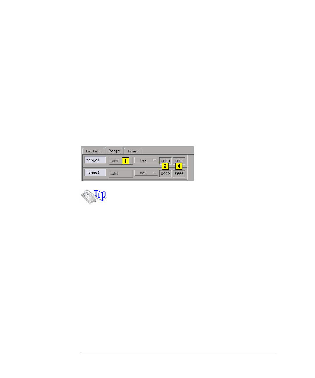
Chapter 1: HP 16554A 70 MHz State/500 MHz Timing Logic Analyzer

The Trigger Tab

To Define a Range Term

1. Click the label name to the right of the term name and choose the label

that you want to use. Only one label can be used at a time for range terms.

2. Click the lower value field, to the right of the label name.

3. Type the pattern for the low value of the range.

4. Click the upper value field, to the right of the label name.

5. Type the pattern for the upper value of the range. Depending on the base setting, such as Hex or Octal, some characters will not be accepted.

Right-click on either of the value fields to quickly assign the value to a preset value. Set (=1) sets the value to all 1s. Reset (=0) sets the value to all 0s.

Using Edge Terms

Edge terms are only available in timing mode. You can set an edge term to match transitions or glitches on one or more channels. When you specify an edge or glitch on more than one channel, the analyzer logically ORs the edges together. When the analyzer sees a transition that matches any of the ones specified in the edge term, the term becomes true. If you must have both edges occur in the same sample, assign the edges to different terms and combine them (see page 84) with an AND.

The following edge choices are available for each bit:

Rising edge (*)

Chapter 1: HP 16554A 70 MHz State/500 MHz Timing Logic Analyzer

The Trigger Tab

Falling edge (*)

Either rising or falling

Glitch (*)

To Define an Edge Term

1. Click the label name and choose the label that you want to use.

2. Click the edge value field, to the right of the label name.

3. Set the edge or glitch for each channel. Don’t cares are indicated by a (.).

NOTE: After you close the edge term assignment dialog, you may see $ indicators in

the term value field. This symbol indicates that the value can’t be displayed in the selected base. Choose Binary base to see the actual assignments.

Using Timer Terms

Timers are like other resource terms in that they are either true or false. They are unlike other terms, however, in that they are controlled within the trigger sequence and act like a stopwatch. When a timer reaches its assigned count (expires), it becomes true. When a timer expires or stops, its count resets to zero.

Timers can be set to Start, Stop, Pause, or Continue as the analyzer enters a trigger sequence level. The two timers are global, so each sequence level except the first has the ability to control the same timer. As more sequence levels are added, the timer status in the new levels defaults to Off. If a timer is paused in one level, it must be continued in another level before it will be restarted. If the trigger sequence returns to the same sequence level again, the timer will be restarted.

Each Timer term can be used by either of the two analyzers, but not both.

To Assign a Time Value to the Timer Terms

1. Click the Timer tab in Trig g e r.

2. Click in the timer value field, next to the timer name.

Chapter 1: HP 16554A 70 MHz State/500 MHz Timing Logic Analyzer

The Trigger Tab

3. Type in a timer value.

4. Use the up/down arrow buttons to scroll through timer values.

The minimum value a timer can have is 400 ns, which is also the default value.

To Include a Timer in a Trigger Sequence

1. Assign a time value to the timer you want to use.

2. Click the sequence level you want to use it in, and select Edit....

Timer control is not available in the first sequence level.

3. Click Off at the bottom of the edit dialog box and select Start.

If the other analyzer is already using a timer, it won’t appear in this analyzer’s edit dialog.

4. Click the event field where you want to use the timer.

5. Select either Timer or Combo....

Use Combo for cases such as an edge occurring after so many nanoseconds.

6. In the other trigger levels, you can Start, Pause, and Continue the timer. When a timer reaches its assigned value, it automatically stops.

See Also “Using Combinations of Terms” on page 84

Using Combinations of Terms

Resource terms can be used in combinations. Combinations use the logical AND, NAND, OR, NOR, and XOR functions to combine predefined resource terms.

A combined term is evaluated as a single events. Components that are ANDed together must all occur in the same sample. Ones that are ORed together only require one of the components to happen.

If you intend for the logic analyzer to decide between two actions, use branches instead of combined terms. If you want the logic analyzer to find the terms in sequence, use different levels or a trigger function in the trigger sequence.

Chapter 1: HP 16554A 70 MHz State/500 MHz Timing Logic Analyzer

The Trigger Tab

To Set Up a Combination

1. Edit the sequence step (see page 65) that you want a combination term to appear in.

2. Click on the resource term assignment field that you want to make into a combination.

3. Choose Combo... from the menu of resource terms.

4. In the Combination dialog, click the On/Off/Not button for each term that you want to use and select On or Not. Not selects the logical negation of the term.

5. Click the logical operator buttons and choose a logic operation. Not all operations are available at all levels of the combination tree.

NOTE: The combination of terms is now inserted into the term assignment field. If the

term is too long to fit, the display is truncated.

Adding and Deleting Labels for Terms

Labels are defined in Format, after which they are available throughout the other analyzer areas and attached display tools.

When you use more than one label to define a trigger term, the term conditions must be true on both labels for the term to be true.

To Add a Label to a Resource Term

1. Click the label name.

2. Select Insert.

3. Select the label that you want to add to the resource term.

To Delete a Label from a Resource Term

1. Click the label name.

2. Select Delete.

Numeric Base

All labels have a numeric base field next to them. The base choices are

Chapter 1: HP 16554A 70 MHz State/500 MHz Timing Logic Analyzer

The Trigger Tab

Binary, Octal, Decimal, Hex, ASCII, Symbol and Twos Complement.

To Change the Numeric Base

1. Click the base button.

2. Choose the base that you want.

NOTE: If the numeric base is changed in one window, the base in other windows may

not change accordingly. For example, the base assigned to symbols is unique, as is the base assigned in the Listing window.

Tagging Data with Time or State Tags (State Only)

The Count field under Settings in Trig g e r accesses a selection menu which is used to stamp the data at each memory location with either a Time tag or a State Count tag. The tags reduce the memory depth by half. To retain the full memory depth when using time or state tags leave one pod pair unassigned.

State Count

When the State Count option is selected, numbered tags are placed on all selected data. Pre-trigger data has negative numbers and posttrigger data has positive numbers. You select the data to be tagged when you turn on State Count. A field appears to the right of States that lets you define patterns.

State tag numbering can be set either relative to the previous tagged sample or absolute from the trigger point. Selecting Absolute or Relative is done by toggling the Absolute/Relative field in the Listing Display window.

Time Count

Time Count places time tags on all data. Pre-trigger data has negative time numbers and post-trigger data has positive time numbers. Time tag numbering is set to be either relative to the previous memory location or absolute from the trigger point. The time tag resolution is 4

Chapter 1: HP 16554A 70 MHz State/500 MHz Timing Logic Analyzer

The Trigger Tab

ns.

Arming Control

An instrument must be armed before it can look for its trigger. When you Run an instrument, it is armed immediately. When using logic analyzer modules that provide two separate analyzers, you can set one analyzer to arm the other within the same module by selecting Arming Control... under Settings in Tr i gge r.

Clicking Arming Control... brings up the Machine Arming Tree dialog. In this dialog you can set what starts each analyzer, and which one sends a signal to Arm Out. Arm Out is used to send signals to other instruments in the frame, or sent to Port Out. Port Out can be used to control additional instruments external to the logic analysis system.

To change the source of Arm In or the destination of Port Out, use the Intermodule dialog (see the HP 16600A/16700A Logic Analysis System help volume).

Setting One Analyzer to Arm the Other

This procedure assumes you have both analyzers turned on. The second analyzer can be turned on by dragging it onto the workspace in the Workspace window.

1. Under Trigger, click Settings.

2. Click Arming Control....

3. Click the box of the machine that you want to have wait for its arm signal.

4. In the armed by menu, select the other machine. The arming signal path forms a tree in the Machine Arming Tree dialog.

5. Set the sequence level number to the trigger sequence level that will wait for the arm signal. It does not have to be the same as the trigger level.

6. Click Close.

Chapter 1: HP 16554A 70 MHz State/500 MHz Timing Logic Analyzer

The Trigger Tab

NOTE: If the trigger sequence does not pass through the level containing the wait for

arm term, the trigger will not wait for the arming signal.

See Also Overview - Multiple Instrument Configuration (see the HP 16600A/

16700A Logic Analysis System help volume)

Overview - Multiple Machine Configuration (see the HP 16600A/16700A Logic Analysis System help volume)

Chapter 1: HP 16554A 70 MHz State/500 MHz Timing Logic Analyzer

Specifications and Characteristics

NOTE: Definition of Terms To understand the difference between specifications (see

page 89) and characteristics (see page 89), and what gets a calibration procedure (see page 90) and what gets a function test (see page 90), refer to appropriate links within this note.

“HP 16554A Logic Analyzer Specifications” on page 90

“HP 16554A Logic Analyzer Characteristics” on page 91

What is a Specification

A Specification is a numeric value, or range of values, that bounds the performance of a product parameter. The product warranty covers the performance of parameters described by specifications. Products shipped from the factory meet all specifications. Additionally, the products sent to HP Customer Service Centers for calibration and returned to the customer meet all specifications.

Specifications are verified by Calibration Procedures.

What is a Characteristic

Characteristics describe product performance that is useful in the application of the product, but that is not covered by the product warranty. Characteristics describe performance that is typical of the majority of a given product, but not subject to the same rigor associated with specifications.

Characteristics are verified by Function Tests.

Chapter 1: HP 16554A 70 MHz State/500 MHz Timing Logic Analyzer

Specifications and Characteristics

What is a Calibration Procedure

Calibration procedures verify that products or systems operate within the specifications. Parameters covered by specifications have a corresponding calibration procedure. Calibration procedures include both performance tests and system verification procedure. Calibration procedures are traceable and must specify adequate calibration standards.

Calibration procedures verify products meet the specifications by comparing measured parameters against a pass-fail limit. The pass-fail limit is the specification less any required guardband.

The term "calibration" refers to the process of measuring parameters and referencing the measurement to a calibration standard rather than the process of adjusting products for optimal performance, which is referred to as an "operational accuracy calibration".

What is a Function Test

Function tests are quick tests designed to verify basic operation of a product. Function tests include operator’s checks and operation verification procedures. An operator’s check is normally a fast test used to verify basic operation of a product. An operation verification procedure verifies some, but not all, specifications, and often at a lower confidence level than a calibration procedure.

HP 16554A Logic Analyzer Specifications

The specifications are the performance standards against which the product is tested. These specifications apply only to the HP 16554A 70 MHz State/500 MHz Timing logic analyzer:

Minimum State Clock Pulse Width: 3.5 ns Threshold Accuracy: +/- (100mV + 3% of threshold setting) Minimum Master-to-Master Clock Time: 10.0 ns Setup/Hold Time:

Chapter 1: HP 16554A 70 MHz State/500 MHz Timing Logic Analyzer

Specifications and Characteristics

*Single Clock, Single Edge: 0.0/3.5 ns through 3.5/0.0 ns, adjustable in 500-ps increments *Single Clock, Multiple Edge: 0.0/4.0 ns through 4.0/0.0 ns, adjustable in 500-ps increments *Multiple Clock, Multiple Edge: 0.0/4.5 ns through 4.5/0.0 ns, adjustable in 500-ps increments

* Specified for an input signal VH=-0.9 V, VL=-1.7 V, threshold=-1.3 V, slew rate=1 V/ns

HP 16554A Logic Analyzer Characteristics

The characteristics are not specifications, but are included as additional information.

General Information

- Channel Counts:

1-card module 64 data/4 clock 2-card module 132 data/4 clock 3-card module 200 data/4 clock

- Memory Depth:

Half Channel 1 Msamples Full Channel 500 Ksamples

Probes

- Input Resistance: 100 Kohm, +/- 2%

- Input Capacitance: ~8 pF

- Minimum Voltage Swing: 500 mV peak-to-peak

- Maximum Voltage: +/- 40 V peak, CAT I

- Threshold Range: +/- 6.0 V, adjustable in 50-mV increments

- Power through pod cables: 1/3 amp at 5 V maximum per pod

State Analysis

- Maximum State Clock Speed: 70 MHz

- State Clocks: 4

- State Clock Qualifiers: 4

Each qualifier can be set to recognize one of six clock lines, either high or low.

- Time Tag Resolution: 8 ns

- Maximum Time Count Between States: 34 seconds

**Minimum times are given for an input signal VH=-0.9 V, VL=-1.7 V, threshold=-1.3 V, slew rate=1 V/ns

Timing Analysis

- Maximum Conventional Timing Rate:

Half Channel 250 MHz Full Channel 125 MHz

- Sample Period Accuracy: 0.01% of sample period

- Channel-to-Channel Skew: 2 ns, typical

- Time Interval Accuracy: +/-( sample period + channel-to-

channel skew + 0.01% of time interval reading )

Triggering

- State Sequence Levels: 12

- Timing Sequence Levels: 10

- Maximum Occurrence Count Value: 1,048,575

- Pattern Recognizers: 10

- Range Recognizers: 2

- Range Width: 32 bits each

- Timers: 2

Chapter 1: HP 16554A 70 MHz State/500 MHz Timing Logic Analyzer

Specifications and Characteristics

- Timer Value Range: 400 ns to 500 seconds

- Glitch/Edge Recognizers: 2 (timing only)

- Minimum Detectable Glitch: 3.5 ns

Power Requirements All necessary power is supplied by the backplane connector of the logic analysis system mainframe.

Operating Environment Characteristics

- Indoor use only.

- Temperature Instrument (except disk and media): 0 to 55 degrees C (+32 to 131 degrees F) Probe lead sets and cables: 0 to 65 degrees C (+32 to 149 degrees F)

- Humidity Instrument, probe lead sets, and cables: up to 95% relative humidity at 40 degrees C (+122 degrees F)

- Altitude To 4600 m (15,000 ft)

- Vibration Operating: Random vibration 5 to 500 Hz, 10 minutes per axis,

0.3 g (rms) Nonoperating: Random vibration 5 to 500 Hz, 10 minutes per axis, approximately 2.41 g (rms); and swept sine resonant search, 5 to 500 Hz, 0.75 g (0-peak), 5-minute resonant dwell at 4 resonances per axis.

Chapter 1: HP 16554A 70 MHz State/500 MHz Timing Logic Analyzer

Analyzer Probing Overview

The figures below shows a variety of simple probing connections. The specific probe type, number of probes, and location on the target circuit depends on your particular measurement.

For equivalent circuit diagrams and pinouts, see the description of the probe type in the Logic Analysis System and Measurement Modules

Installation Guide. If you have misplaced the Logic Analysis System and Measurement Modules Installation Guide, you can download

the latest version from the Web at <URL: http://www.hp.com/go/ LogicAnalyzer-Manuals/ >

Probe Lead-to-Board Connection

The standard lead set plugs directly into any .1-inch grid with 0.026 to

0.033-inch diameter round pins or 0.025-inch square pins. All probe

tips work with the HP 5059-4356 surface mount grabbers and the HP 5959-0288 through-hole grabbers.

Chapter 1: HP 16554A 70 MHz State/500 MHz Timing Logic Analyzer

Analyzer Probing Overview

Adapter-to-Board Connection

Both the 01650-63203 and the E5346A adapters include termination for the logic analyzer. The 01650-63203 termination adapter plugs into a 2 x 10 pin header with 0.1 inch spacing. The E5346A high-density adapter connects to an AMP "Mictor 38" connector. If possible, use support shrouds around the Mictor connector to relieve strain and improve connections.

Direct Pod-to-Board Connection

If you provide proper termination as part of the target board, you can plug the pod directly into the ©3M 2520-series, or similar alternative connector. Suggested termination is shown in the Logic Analysis System and Measurement Modules Installation Guide.

Also use this termination with the HP E5351A high-density, nonterminated adapter.

Pod-to-Analysis Probe Connection

Analysis probes (formerly called preprocessors) are microprocessorspecific interfaces that make it easier to probe buses. Generally,

Chapter 1: HP 16554A 70 MHz State/500 MHz Timing Logic Analyzer

Analyzer Probing Overview

analysis probes consist of a circuit board that attaches to the microprocessor (possibly through an adapter) and a configuration file. The configuration file sets up the logic analyzer’s clocks and labels correctly, and may include an inverse assembler. The circuit board provides access to logical groups of pins through headers designed to connect directly to the logic analyzer.

The easiest way to set up a measurement with an analysis probe is the Setup Assistant. (see the Setup Assistant help volume) The Setup Assistant asks you questions about your measurement and then shows you just the information you need to set up the probe correctly. It also loads the proper configuration files.

Chapter 1: HP 16554A 70 MHz State/500 MHz Timing Logic Analyzer

The Symbols Tab

The Symbols tab offers control of the symbols capabilities. Symbols represent patterns and ranges of values found on labeled sets of bits. Two kinds of symbols are available:

• Object File Symbols. These are symbols from your source code and symbols generated by your compiler.

• User-Defined Symbols. These are symbols you create.

To load symbols, click one of the following:

•“To Load Object File Symbols” on page 98

•“To Load User-Defined Symbols” on page 110

Symbols are available for all state and timing analyzers. Each label listed in the Format menu can have its own group of symbols associated with it.

•“User-Defined Symbols” on page 109

•“Setting Up Object File Symbols” on page 98

•“Using Symbols In The Logic Analyzer” on page 111

•“Displaying Data in Symbolic Form” on page 97

Chapter 1: HP 16554A 70 MHz State/500 MHz Timing Logic Analyzer

Displaying Data in Symbolic Form

You can display data in symbolic form in some of the display tools, such as the Listing display and the Waveform display.

To View Symbolic Values in a Waveform Display

1. Right-click the label name where you want to display symbolic values.

2. Select Change attributes....

3. In the Attribute Dialog:

• Set ShowValue to On.

• Set Base to Symbols or Line#.

• Click OK.

The symbolic names for the values now appear in the overlayed bus waveform.

To View Symbolic Values in a Listing Display

1. Right-click the numeric base of the label where you want to display symbolic values.

2. Set the numeric base to Symbols or Line#. The symbolic names for the values now appear instead of numeric data.

Chapter 1: HP 16554A 70 MHz State/500 MHz Timing Logic Analyzer

Setting Up Object File Symbols

Object file symbols can include variable names, procedure or function names, and source file names with line numbers. The linkage between symbol names and address or data values comes from one of two sources:

• Object files that are created by your compiler/linker.

• ASCII symbol files you create with a text editor.

To use object file symbols

1. Generate an object file with symbolic information using your software development tools.

2. If your language tools cannot generate object file formats that are supported by the logic analyzer, create an ASCII symbol file (see page 102).

3. Load the object file (see page 98) or ASCII symbol file into the logic analyzer.

4. If necessary, relocate sections of your code (see page 100).

See Also “Using Symbols In The Logic Analyzer” on page 111

“Symbol File Formats” on page 101

To Load Object File Symbols

1. Select the Symbol tab and then the Object File tab.

2. Select the label name you want to load object file symbols for. In most cases you will select the label representing the address bus of the processor you are analyzing.

3. Specify the directory to contain the symbol database file (.ns ) in the field under, Create Symbol File (.ns) in This Directory. Click Browse... if you wish to find an existing directory name.

Chapter 1: HP 16554A 70 MHz State/500 MHz Timing Logic Analyzer

Setting Up Object File Symbols

4. In the Load This Object/Symbol File For Label field, enter the object file name containing the symbols. Click Browse... to find the object file and click Load in the Browser dialog. If your logic analyzer is NFS mounted to a network, you can select object files from other servers.

To reload object file symbols

1. Select the object file/symbol file to reload from the Object Files with Symbols Loaded For Label field.

2. Click the Reload button.

Value update

The values of the object file symbols being used as terms or as SPA state-interval ranges will be updated automatically each time the object file symbols are reloaded.

Configuration file save

The name of the current object file is saved when a configuration file is saved. The object file will be reloaded when the configuration is loaded.

Multiple files

You can load the same symbol file into several different analyzers, and you can load multiple symbol files into one analyzer. Symbols from all the files you load will appear together in the object file symbol selector that you use to set up resource terms.

Object file versions

During the load process, a symbol database file with a .ns extension will be created by the system. One .ns database file will be created for each symbol file you load. Once the .ns file is created, the Symbol Utility will use this file as its working symbol database. The next time you need to load symbols into the system, you can load the .ns file explicitly, by placing the .ns file name in the Load This Object/Symbol File For Label field.

If you load an object file that has been loaded previously, the system will compare the time stamps on the .ns file and the object file. If the

Chapter 1: HP 16554A 70 MHz State/500 MHz Timing Logic Analyzer

Setting Up Object File Symbols

object file is newer, the .ns file will be created. If the object file has not been updated since it was last loaded, the existing .ns file will be used.

See Also “Using Symbols In The Logic Analyzer” on page 111

“Symbol File Formats” on page 101

Relocating Sections of Code

Use this option to add offset values to the symbols in an object file. You will need this if some of the sections or segments of your code are relocated in memory at run-time. This can occur if your system dynamically loads parts of your code so that the memory addresses that the code is loaded into are not fixed.

To Relocate a Single Section of Code

1. Click the Symbol tab and then the Object File tab.

2. In the Object Files with Symbols Loaded For Label list, select the file

whose symbols you wish to relocate.

3. Select the Relocate Sections... button.

4. In the Section Relocation dialog, click the field you wish to edit in the

section list.

5. Type in the new value for that field and press Enter on your keyboard.

6. Repeat steps 4 through 6 above for any other sections to be relocated.

7. Click Close.

To Relocate All Sections of Code

1. Click the Symbol tab and then the Object File tab.

2. In the Object Files with Symbols Loaded For Label list, select the file

whose symbols you wish to relocate.

3. Select the Relocate Sections... button.

4. Type the desired offset in the Offset all sections by field. The offset is

100

Agilent 16554A Help Volume

Specifications and Main Features

Frequently Asked Questions

User Manual

Contents

Setting Up a Measurement

Connect the Analyzer to the Target System

Define the Type of Measurement

Set Up the Bus Labels

Define Trigger Conditions

Run the Measurement

Examine the Data

Making a Basic State Measurement

Making a Basic Timing Measurement

Interpreting the Data

Analysis Using Waveform

Analysis Using Listing

Coordinating Measurements

Loading and Saving Logic Analyzer Configurations

When Something Goes Wrong

Interference with Target System

Error Messages

Nothing Happens

Suspicious Data

Maximum of 32 Channels Per Label

Measurement Initialization Error

Slow or Missing Clock

Timer is Specified in Sequence, But Never Started

Timer is off in sequence level where it is used

Trigger inhibited during timing prestore

Two Pod Pairs are Needed To Use Both Timers

Waiting for Trigger

Incompatible Data Not Loaded

Incompatible Timing Data Not Loaded

Incompatible Time Tags Not Loaded

Measurement Error: Check Probe Parametrics or Grounding

Tag Data Has Been Discarded

Cannot Read Unrecognized Data

Testing the Logic Analyzer Hardware

The Sampling Tab

Acquisition Depth

Setting the Acquisition Mode

Performing Clock Setup (State only)

Clock Modes (State only)

Naming the Analyzer

Turning the Analyzer Off

Sample Period (Timing Only)

State Acquisition Modes

Timing Acquisition Modes

Trigger Position Control

The Format Tab

Activity Indicators

Assigning Pods to the Analyzers

Data On Clocks Display

Assigning Bits to a Label

Inserting and Deleting Labels

Turning Labels On and Off

Label Polarity

Reordering the Bits in a Label

Labels: Mapping Analyzer Channels to Your Target

Setting Up the Pod Clock

Pod Selection

Setting the Pod Threshold

State Clock Setup/Hold (State only)

The Trigger Tab

Understanding Logic Analyzer Triggering

Setting Up a Trigger

Selecting a Function to Match Trigger Conditions

Inserting and Deleting Sequence Steps

Editing Sequence Steps

Setting Up Loops and Jumps in the Trigger Sequence

Saving and Recalling Trigger Sequences

Clearing Part or All of the Trigger

Overview of the Trigger Sequence

Trigger Functions

Timing User Level

Basic Timing Trigger Functions

Pattern/Edge Combinations

Time Vi olat ions

State User-level