Agilent 0A Operator Datasheet

Download

Page 1

Agilent 35670A Operator’s Guide

Agilent Part Number 35670-90053 For instruments with firmware version A.00.00 Printed in U.S.A.

Page 2

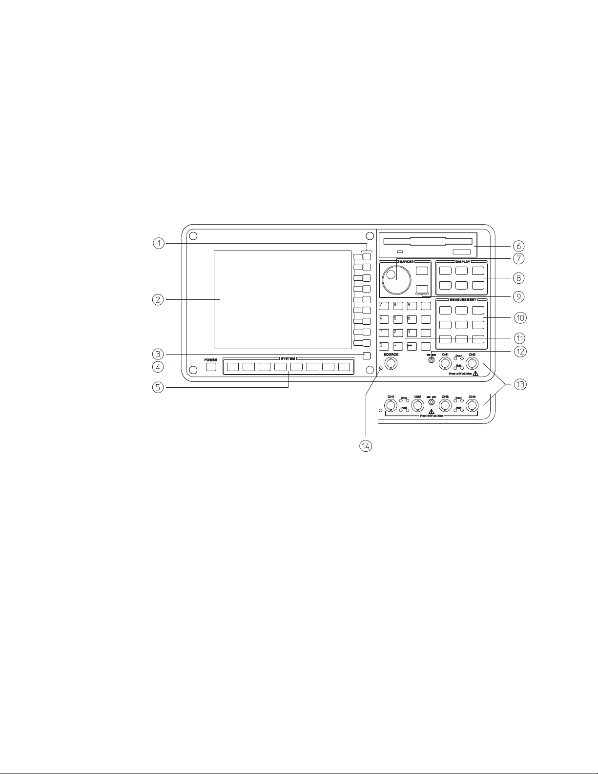
The Agilent 35670A at a Glance (Front Panel)

Page 3

Agilent 35670A Front Panel

1-Use the softkeys to select items from the current

menu. A softkey’s function is indicated by a video label on the analyzer’s screen. Throughout this book, softkeys are printed like this: [

FFT ANALYSIS

Hardkeys are front-panel buttons whose functions are always the same. They have a label printed directly on the key itself. Throughout this book, hardkeys are printed like this: [

Inst Mode

2-The analyzer’s screen is divided into the menu

area and the display area. The menu area displays video labels for the softkeys. The data area displays measurement data and information about the parameter settings.

3-The [

level.

] key returns the menu to the previous

Rtn

4-The POWER switch turns on the analyzer.

5-Use the SYSTEM keys to control various

system-level functions. These functions include saving files, plotting measurement data, and accessing online help.

6-Use the disk drive to save your work on 3.5

inch flexible disks.

7-The knob moves the markers and the cursor. It

also steps through numeric values and scrolls through online help.

10-Use the MEASUREMENT keys to control the

analyzer’s source and inputs. They also control measurement parameters. You must make a new

measurement if you change a MEASUREMENT parameter.

11-Use the numeric-entry keys to enter a numeric

value.

12-The microphone power connector provides

power (8 Vdc) for the Microphone Adapter Kit (Option UK4).

13-The connector area of the front panel has two

different configurations. The standard analyzer has a source output connector and two input connectors. The 4-channel analyzer (Option AY6) has four input connectors.

Range indicators are located next to each input connector. The upper LED is the over-range indicator (the signal level exceeds the current range setting). The lower LED is the half range indicator (the signal level exceeds half the current range setting).

14-A source on/off indicator is located at the left

edge of the connector area.

The standard Agilent 35670A (2-channel) has a source connector on the front panel.

8-Use the DISPLAY keys to control what

appears on the analyzer’s traces. They only affect how data is displayed; DISPLAY keys do not change measurement parameters. You can press

keys in the DISPLAY menus without losing measurement parameters.

9-Use the MARKER keys to select a variety of

marker features.

Page 4

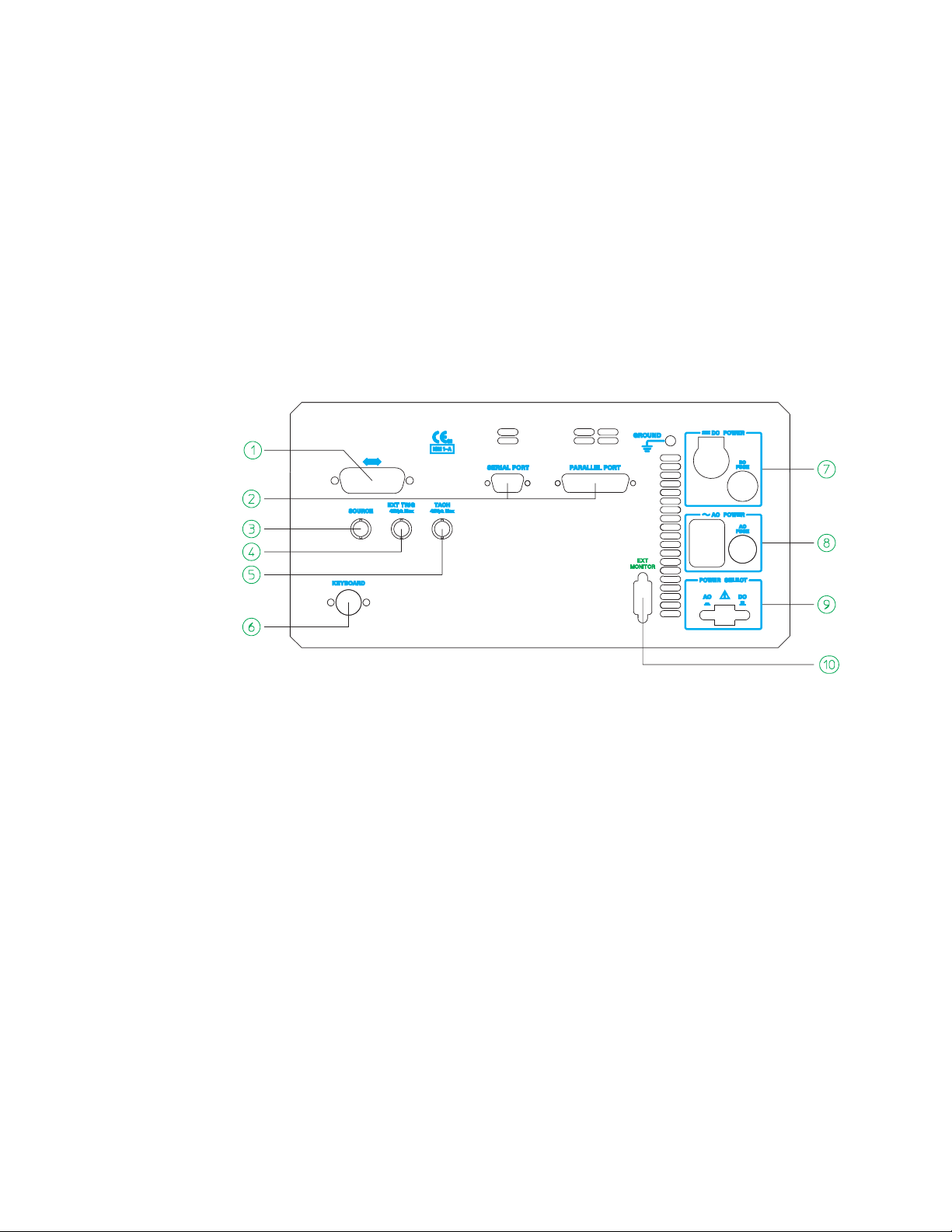
The Agilent 35670A at a Glance (Rear Panel)

Page 5

Agilent 35670A Rear Panel

1-The GPIB connector links the Agilent 35670A

to other GPIB devices. GPIB parameters are set in the [

Local/GPIB

] and [

Plot/Print

] menus.

2-The SERIAL PORT and the PARALLEL

PORT link the analyzer to plotters and printers. These parameters are set in the [

Plot/Print

] menu.

3-The SOURCE connector outputs the analyzer’s

source signal. An LED on the front panel indicates if the source is on or off. The source parameters are set in the [

The standard Agilent 35670A (2-channel) also has a source connector on the front panel.

Source

] menu.

4-The EXT TRIG connector links the analyzer to

an external trigger signal. The external trigger parameters are set in the [

Trigger

] menu.

5-The TACH connector links the analyzer to a

tachometer. The tachometer parameters are set in the [

Input

] menu.

6-The KEYBOARD connector attaches an

optional keyboard to the analyzer.

7-The DC POWER connector accepts DC power

levels from 12 - 28 Vdc (nominal).

8-The AC POWER connector accept a wide range

of ac voltage levels.

9-The POWER SELECT switch determines

whether the analyzer is powered via the AC POWER connector or the DC POWER connector.

10-The EXT MONITOR port links the analyzer

to multi-sync monitors.

Page 6

Page 7

Saftey Summary

The following general safety precautions must be observed during all phases of operation of this instrument. Failure to comply with these precautions or with specific warnings elsewhere in this manual violates safety standards of design, manufacture, and intended use of the instrument. Agilent Technologies, Inc. assumes no liability for the customer’s failure to comply with these requirements.

GENERAL

This product is a Safety Class 1 instrument (provided with a protective earth terminal). The protective features of this product may be impaired if it is used in a manner not specified in the operation instructions.

All Light Emitting Diodes (LEDs) used in this product are Class 1 LEDs as per IEC 60825-1.

ENVIRONMENTAL CONDITIONS

This instrument is intended for indoor use in an installation category II, pollution degree 2 environment. It is designed to operate at a maximum relative humidity of 95% and at altitudes of up to 2000 meters. Refer to the specifications tables for the ac mains voltage requirements and ambient operating temperature range.

BEFORE APPLYING POWER

Verify that the product is set to match the available line voltage, the correct fuse is installed, and all safety precautions are taken. Note the instrument’s external markings described under Safety Symbols.

GROUND THE INSTRUMENT

To minimize shock hazard, the instrument chassis and cover must be connected to an electrical protective earth ground. The instrument must be connected to the ac power mains through a grounded power cable, with the ground wire firmly connected to an electrical ground (safety ground) at the power outlet. Any interruption of the protective (grounding) conductor or disconnection of the protective earth terminal will cause a potential shock hazard that could result in personal injury.

Page 8

FUSES

Only fuses with the required rated current, voltage, and specified type (normal blow, time delay, etc.) should be used. Do not use repaired fuses or short-circuited fuse holders. To do so could cause a shock or fire hazard.

DO NOT OPERATE IN AN EXPLOSIVE ATMOSPHERE

Do not operate the instrument in the presence of flammable gases or fumes.

DO NOT REMOVE THE INSTRUMENT COVER

Operating personnel must not remove instrument covers. Component replacement and internal adjustments must be made only by qualified service personnel.

Instruments that appear damaged or defective should be made inoperative and secured against unintended operation until they can be repaired by qualified service personnel.

WARNING The WARNING sign denotes a hazard. It calls attention to a procedure,

practice, or the like, which, if not correctly performed or adhered to, could result in personal injury. Do not proceed beyond a WARNING sign until the indicated conditions are fully understood and met.

Caution The CAUTION sign denotes a hazard. It calls attention to an operating

procedure, or the like, which, if not correctly performed or adhered to, could result in damage to or destruction of part or all of the product. Do not proceed beyond a CAUTION sign until the indicated conditions are fully understood and met.

Page 9

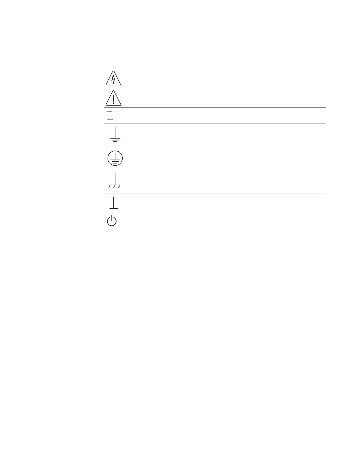
Safety Symbols

Warning, risk of electric shock

Caution, refer to accompanying documents

Alternating current

Both direct and alternating current

Earth (ground) terminal

Protective earth (ground) terminal

Frame or chassis terminal

Terminal is at earth potential.

Standby (supply). Units with this symbol are not completely disconnected from ac mains when

this switch is off

Page 10

Page 11

Table of Contents

Part I Making Measurements

Setting Up a Measurement Part I-1

1 Measuring Rotating Machinery

To connect transducers 1-2

To specify a transducer’s unit and sensitivity 1-3

To calibrate a transducer 1-4

To measure vibration power 1-6

To characterize a tachometer signal 1-8

To measure an order spectrum 1-10

To display an rpm-stepped order map 1-12

To display a time-stepped order map 1-13

To measure an order track 1-14

To display an rpm-stepped order track 1-16

To display a time-stepped order track 1-17

To display phase relative to the tachometer signal 1-18

To display an rpm profile 1-19

To display an orbit diagram 1-20

2 Measuring Structures

Measuring Structures 2-2

Impact Testing 2-8

To measure a driving point measurement 2-10

To view unwrapped phase of a driving point measurement 2-12

To view the real and imaginary components of a driving point

measurement 2-13

To preview the time record 2-14

Page 12

3 Measuring Sound

To connect the microphone adapter (Option UK4) 3-2

To connect microphones 3-3

To calibrate a microphone 3-4

To measure sound pressure level 3-6

To measure overall sound pressure level 3-8

To measure overall impulse characteristics 3-9

4 Measuring Spectra and Networks

To measure a wideband spectrum 4-2

To measure a narrowband spectrum 4-4

To measure frequency and amplitude 4-5

To measure noise power (PSD) 4-6

To measure harmonic distortion 4-7

To measure sideband power 4-8

To display a spectral map 4-9

To measure frequency response—FFT 4-10

To measure frequency response—swept sine 4-12

To measure phase distortion 4-14

5 Measuring Control Systems

Measuring Control Systems 5-2

Measuring Control System Performance 5-6

To measure a step response 5-8

To measure performance parameters 5-10

Measuring Control System Stability 5-12

To measure an open loop response 5-14

To measure gain and phase margin 5-16

To display a Nyquist diagram. 5-17

To measure a closed loop response 5-18

To calculate the open loop response 5-20

6 The Arbitrary Source Option 1D4

The Arbitrary Source 6-2

To create a step signal 6-4

To create a ramp signal 6-6

To create a profiled chirp waveform 6-8

Page 13

7 Using Time Capture

To prepare for filling the capture buffer 7-2

To allocate memory for the capture buffer 7-4

To fill the capture buffer 7-5

To save the capture buffer on a flexible disk 7-6

To recall a capture buffer from a flexible disk 7-7

To examine the capture buffer 7-8

To define an analysis region 7-9

To prepare for measuring from the capture buffer 7-10

To measure from the capture buffer 7-12

Part II Working with the Display

8 Displaying Measurement Data

To select the active trace 8-2

To display measurement data—one channel, one trace 8-3

To display measurement data—one channel, multiple traces 8-4

To display measurement data—multiple channels, multiple traces 8-5

To display a data register 8-6

To display a math function 8-7

9 Formatting the Display

To arrange traces on the screen 9-2

To enable global screen elements 9-3

To enable trace-specific screen elements 9-4

To enter your own trace title 9-5

To control the screen 9-6

To set up a waterfall display 9-7

To enhance a waterfall display 9-8

To display the waterfall buffer 9-9

To display one trace from the waterfall buffer 9-10

To display a slice through the waterfall buffer 9-11

Page 14

10 Scaling the Display

To enable Y-axis autoscaling 10-2

To scale the Y-axis with Reference and Y Per Div softkeys 10-3

To set top and bottom values for the Y-axis 10-4

To scale the Y-axis with axes scale markers 10-5

To match Y-axis scaling of another trace 10-6

To scale the X-axis with axes scale markers 10-7

To match X-axis scaling of another trace 10-8

11 Selecting Display Units

To select a coordinate system 11-2

To select the frequency/time unit 11-3

To select the phase unit 11-4

To select the amplitude unit 11-5

To specify a transducer’s unit and sensitivity 11-6

To convert a displayed transducer unit 11-7

To display amplitude in dBm 11-8

Part III Using the Basics

12 Using Online Help

Todisplayhelpforakey12-2

To display a related help topic 12-3

To select a topic from the help index 12-4

To print a help topic 12-5

To exit the help system 12-6

Page 15

13 Managing Files and Disks

Tosetupanexternaldisk13-2

To select the default disk 13-3

To format a flexible disk 13-4

To change the current DOS directory 13-5

To create a DOS directory 13-6

Tosaveatrace13-7

To save a program 13-8

To save other data 13-9

To recall a trace 13-10

To recall a program 13-11

To recall other data 13-12

To delete a file 13-13

To delete a DOS directory 13-14

To copy a file 13-15

To rename a file 13-16

14 Plotting and Printing

To set up your hardcopy device—parallel 14-2

To set up your hardcopy device—serial 14-3

To set up your hardcopy device—HP-IB 14-4

To plot screen contents 14-5

To print screen contents 14-6

To annotate a plot or print 14-7

To reassign plotter pens 14-8

To modify the plotting speed 14-9

To position a plot on the page 14-10

Page 16

Part IV Using Advanced Tools

15 Synthesis Option 1D3

Synthesis 15-2

The Synthesis Table and Data Formats 15-4

To display a synthesis table — Pole-Zero Format 15-15

To select/convert a table format — Pole-Residue format 15-16

To select/convert a table format — Polynomial format 15-17

Creating a Synthesis Table 15-18

To create a synthesis table 15-22

To clear a synthesis table 15-24

Performing the Synthesis 15-25

To synthesize a frequency response curve 15-26

To change the data spacing for the X-axis 15-28

Working With Synthesis Tables 15-29

To edit an existing synthesis table 15-30

To save a synthesis table 15-31

To save a synthesis trace 15-32

To recall a synthesis table 15-33

To transfer a curve fit table to a synthesis table 15-34

To change the synthesis register 15-35

16 Curve Fit

Option 1D3

Curve Fit 16-2

Overview of Curve Fit Procedures 16-27

To set up a curve fit 16-30

To specify a weighting function 16-32

To perform a curve fit 16-33

To set up a curve fit — manual operation 16-34

Working with Curve Fit Tables 16-36

To edit a curve fit table 16-37

To transfer a curve fit table to a synthesis table 16-38

compare a frequency response measurement to synthesized results 16-39

To save a curve fit table 16-40

To save a curve fit’s frequency response function 16-41

To recall a curve fit table 16-42

To change the curve fit register 16-43

Page 17

17 Limit Testing

To draw a limit 17-2

To delete a limit segment 17-3

To convert a trace to a limit 17-4

To enable limit testing 17-5

To save a limit 17-6

18 Math Operations and Data Editing

Math Operations and Data Editing 18-2

To define a constant 18-4

To specify an operand within an operation 18-5

To define a function 18-7

To view the results of a math operation 18-8

To compute cepstrum 18-9

To compute a Hilbert transform 18-10

To calculate the envelope of a function 18-11

To compute the signal-to-noise ratio 18-12

To compute group delay 18-13

To modify a waveform 18-14

Page 18

Page 19

Part I

Making Measurements

Page 20

Page 21

Setting Up a Measurement

The following seven chapters present a variety of measurements you can make with the Agilent 35670A and its options. Each chapter focuses on a different type of measurement.

• Rotating Machinery Chapter 1

• Structures Chapter 2

• Sound/Acoustics Chapter 3

• Spectra and Networks Chapter 4

• Control Systems Chapter 5

In addition, the last two chapters show you how to use the analyzer’s optional arbitrary source (chapter 6) and the analyzer’s time capture buffer (chapter 7).

Each measurement follows a basic procedure. Depending upon the measurement, some steps may be eliminated or be revised. Generally, the procedure is as follows:

1 Initialize the analyzer.

2 Make connections.

3 Specify the measurement parameters.

4 Specify the triggering and averaging parameters.

5 Configure the display.

6 Measure the device-under-test (DUT).

In the event that the specific measurement you wish to make is not presented in this book, look for a similar measurement and use the procedure as a guideline. In some cases, the procedure will instruct you to select a preset value. This is done to acquaint you with the menu selections and give you the opportunity to select a different setting.

The following discussion presents an overview of the basic measurement. Detailed information is presented for each step to assist you in making the appropriate selection.

Part I-1

Page 22

Agilent 35670A

Setting Up a Measurement Operator's Guide

Initialize the analyzer

This step initializes the analyzer to a known state, selects the instrument mode and the number of channels, and measurement data.

Preset

Most measurements begin by presetting the analyzer to a known state. this known state provides a convenient starting point when you are setting up a measurement.

Instrument mode / number of channels

When you specify an instrument mode you are asking the analyzer to acquire input data and process it in a certain way. When equipped with a full complement of options, the Agilent 35670A functions as a spectrum analyzer, network analyzer, acoustic sound level meter, acoustic intensity analyzer, vibration analyzer, audio-frequency oscilloscope and amplitude-domain analyzer.

To use each of these different “instruments,” you can press the [

Inst Mode

]

hardkey. Then press the appropriate softkey to select an appropriate instrument mode. The standard Agilent 35670A is equipped with the following instrument modes:

• FFT Analysis

• Correlation Analysis

• Histogram/Time

Additionally, your Agilent 35670A may be equipped with the following optional instrument modes.

• Octave Analysis

• Order Analysis

• Swept Sine

Some measurement features are unavailable with certain instrument modes. (An inactive softkey appears “ghosted.”) Softkey menus change depending on the instrument mode you have selected. The preset instrument mode is FFT analysis.

Part I-2

Page 23

Agilent 35670A Operator's Guide Setting Up a Measurement

The [

Inst Mode

] menu allows you to select the number of channels for your

measurement. The preset selection is a two-channel measurement, set for Channel 1 and Channel 2.

The instrument mode and the number of channels affects the way the analyzer collects input data. (In fact, all the hardkeys in the front panel’s Measurement Group affect the way the analyzer collects input data.) If you change something with any of these keys, the analyzer must retake a measurement.

Measurement data

Each of the six instrument modes has its own set of available measurement data. When you select a type of measurement data, you are instructing the analyzer to display a particular piece of the measurement data that has already been acquired. Measurement data is selected with the [

Meas Data

] hardkey

which is part of the front panel’s Display group. If you press a key in this group, all you are doing is selecting which type of data you want to display—you are not changing the way the analyzer makes measurements.

The following table shows the measurement data available with each instrument mode. For more information about this measurement data, see online help.

Part I-3

Page 24

Agilent 35670A

Setting Up a Measurement Operator's Guide

Measurement data available with each instrument mode

Power Spec

CH1/2/3/4

Linear Spec

CH1/2/3/4

Time

Channel 1/2/3/4

Windowed Time

Chan 1/2/3/4

Frequency

Response 2/1

Frequency

Response 3/1

Frequency

Response 4/1

Frequency

Response 4/3

Coherence 2/1

Coherence 3/1

Coherence 4/1

Coherence 4/3

Cross

Spectrum 2/1

Cross Spectrum

3/1

Cross Spectrum

4/1

Cross Spectrum

4/3

FFT analysis

yes

Octave

Analysis

yes

Order

Analysis

yes

yes yes

yes

†

yes

*†

yes

*†

yes

*†

yes

yes yes

yes

Swept Sine

yes

Correlation

Analysis

yes

Histogram

/Time

‡*

yes

Orbit 2/1

Orbit 3/1

Orbit 4/1

Orbit 4/3

* Channels 3 and 4 available only with Agilent 35670A Option AY6

†

Available only when averaging is turned on

‡

In Histogram/Time mode, time data is called “unfiltered time” data

yes yes

yes

Part I-4

Page 25

Agilent 35670A Operator's Guide Setting Up a Measurement

Measurement data available with each instrument mode (continued)

FFT analysis

Math Function

Data Register

Waterfall

Capture

CH1/2/3/4

Composite

Power CH1/2/3/4

Order Track

CH1/2/3/4

RPM Profile

Normalized

Variance

CH1/2/3/4

Auto

Correlation

CH1/2/3/4

Cross

Correlation 2/1

Cross

Correlation 3/1

Cross

Correlation 4/1

Cross

Correlation 4/3

Histogram

CH1/2/3/4

PDF†CH1/2/3/4

CDF‡CH1/2/3/4

Channels 3 and 4 available only with Agilent 35670A Option AY6

†

Probability Density Function

‡

Cumulative Density Function

Data registers are unique in that they allow you to transport data from one instrument mode to another

Available only when Track is ON in the [

yes yes yes yes yes yes

yes § yes § yes § yes § yes § yes §

yes yes yes yes yes yes

yes

Octave

Analysis

yes

Freq

] menu.

Order

Analysis

yes

Swept Sine

yes

Correlation

Analysis

yes

Histogram

yes

Part I-5

Page 26

Agilent 35670A

Setting Up a Measurement Operator's Guide

Connect the device-under-test/signal source

Each task illustrates the measurement setup. In most cases, the standard two-channel Agilent 35670A is used in the illustration. If you are using a four-channel analyzer (Option AY6), the source connector is located on the rear panel. (The two-channel analyzer has a source connector on both the front and rear panels.)

Set measurement parameters

Measurement parameters affect the way the analyzer takes input data. Most of these selections are grouped under a set of hardkeys in the front panel’s Measurement Group. If you change a parameter under one of these menus you need to take new data.

Specifying frequency data

The Agilent 35670A has a default resolution of 400 lines (401 points, or bins)—and you can specify 800, 200, or 100 lines of display resolution. However, for a given display resolution, narrower spans have finer frequency resolution. This is because the same number of display points represents a smaller range of frequencies.

Full-span measurements let you view the entire frequency spectrum on one display. With the Agilent 35670A, the spectrum can extend from 0 Hz to

102.4 kHz for one-channel measurements, up to 51.2 kHz for two-channel measurements, and 25.6 kHz for four-channel measurements. This provides a frequency resolution, at full-span and 400 lines of resolution, of 256 Hz, 128 Hz, and 64 Hz respectively.

Alternatively, you may wish to view smaller slices of the frequency spectrum. You can select any number of different spans and position these spans where you want by specifying their start or center frequencies. You can also select different spans by specifying a center frequency and a span width. This process of viewing smaller spans is sometimes called “zooming” or “band-selectable analysis.”

Measurements with spans that start at 0 Hz are often called baseband measurements. Those with spans that start at frequencies other than 0 Hz are often called zoomed measurements.

Part I-6

Page 27

Agilent 35670A Operator's Guide Setting Up a Measurement

Frequency Resolution

The frequency resolution of an FFT analyzer is usually stated in number of lines. The most common offerings are 400 and 800 lines, although some analyzers—such as the Agilent 35670A— offer variable resolution. A 400-line FFT analyzer, set up to display a 4 kHz span, would have a frequency resolution of 4000 Hz per 400 lines—10 Hz per line. The length of the time record determines how long a given measurement will take and the maximum frequency that you can measure.

For example, an 800-line analyzer measuring a 1 kHz span requires a 0.8 second time record. A 3200-line analyzer measuring the same 1 kHz span requires a 3.2-second time record. This relationship is

independent of processing speed. The smaller the span, the longer the time record required.

You can easily make calculations to determine values for four inter-related functions; maximum frequency, time-record length, frequency resolution, and frequency span:

• Maximum frequency =

(N/2) x (1/time-record length), where N=number of samples

• Time record length =

number of lines/frequency span

• Frequency resolution = 1/time-record

length

• Frequency span =

(frequency resolution x FFT lines)

Part I-7

Page 28

Agilent 35670A

Setting Up a Measurement Operator's Guide

Configuring the inputs

The standard Agilent 35670A has two input connectors on the front panel. Option AY6 has four input connectors on the front panel. Each input channel is single-ended and has an input impedance of 1 Megohm, shunted by a capacitance of less than 100 pF. When the analyzer is in 1-channel mode, only one input is connected, in 2-channel mode, two inputs are connected, and in 4-channel mode, all four inputs are connected.

Here are some of the different ways to configure each input channel:

• grounded/floating input

• coupling ac/dc

• anti-alias filter on/off

• autoranging on/off

• A-weight filter on/off

• ICP power supply on/off

You can also specify transducer units from the input menu. Transducer units are useful when making measurements with calibrated transducers such as microphones or accelerometers.

In addition, the Agilent 35670A also has a tachometer input and an external trigger input. Both of these connectors are on the rear panel.

Input range

The analyzer has 40 input ranges, from –51 dBVrms to +27 dBVrms in 2 dB increments. You can set the input range manually, or you can use the analyzer’s autoranging feature. If autoranging is on, the analyzer automatically selects a less-sensitive range if the signal exceeds the current input range. To make the best measurement possible, you should carefully consider the method you use to set the input range—setting the range manually or using autorange.

Maximum Input Range (+27dBVrms) and its maximum values in equivalent units

dBVrms dBV(peak) Vrms V(peak)

+27 dBVrms +30.01 dBV(peak) +22.39 Vrms +31.66 V(peak)

Minimum Input Range (–51dBVrms) and its minimum values in equivalent units

dBVrms dBV(peak) Vrms V(peak)

–51 dBVrms –47.99 dBV(peak) +2.818 mVrms +3.986 mV(peak)

Part I-8

Page 29

Agilent 35670A Operator's Guide Setting Up a Measurement

Input overload

The overload status indicators are located next to each input connector. There is also an status message that may appear at the bottom of the analyzer’s display.

If an input channel is currently overloaded the indicator lights up. The status message appears if an input channel is overloaded and the analyzer is unable to change to a less-sensitive range. This occurs if you exceed the analyzer’s maximum input range (+27 dBv). If you turn off autorange, the

message appears anytime you exceed the current input range.

The analyzer’s response to an overload condition varies. If autoranging is on, an overload condition simply causes the analyzer to change to a less-sensitive input range—unless the maximum input range is already selected. If you are making an averaged measurement and an overload occurs, the analyzer begins a new series of averages.

In some cases, the message remains on the display even when there is no longer an overload condition. This lets you know that an overload condition has affected a measurement in progress. Consider this example: you are making an averaged measurement using a fixed input range. At some point during the measurement, an overload occurs. Because the analyzer does not autorange and restart the measurement (because autoranging is off), the message remains to let you know that an overload conditions has corrupted the averaged data.

Caution Although the analyzer’s input has protection circuitry, signals greater than the

following (referenced to ground) may damage the analyzer:

• ± 42 volts (peak) applied to the center conductor of the input connector.

• ± 4 volts (peak) applied to the shell of the input connector (in float mode).

Input overload detection is sensitive to broadband signals—this means that the analyzer senses overload conditions even if the over-range frequency component is outside the analyzer’s current frequency span. Thus the overload status indicators or the status message may appear even if you are viewing a frequency span with no over-range components.

Part I-9

Page 30

Agilent 35670A

Setting Up a Measurement Operator's Guide

Autoranging

When autoranging is on, the analyzer continuously monitors the amplitude of the input signals and, if necessary, automatically changes the input range. If the input signal increases enough to exceed the current input range, the analyzer changes to a less-sensitive input range. When autoranging occurs, the analyzer displays the message. If you are making an averaged measurement and autoranging occurs, the analyzer begins a new series of averages.

You can set the input range manually when you want to maintain a specific input range setting. Ideally, the signal peak should fall in the upper half of the currently-selected input range.

If you set the input range too low (more sensitive than necessary), the analyzer’s input circuitry will introduce distortion into the measurement. But if you set the input range too high (less sensitive than necessary), the resulting loss of dynamic range will introduce additional noise—in some cases, the increase in the noise floor may even obscure low-level frequency components.

If you use a fixed input range, there is approximately 2 dB of headroom at the top of each range before the input channel distorts. So if you are using a fixed input range, an overload condition does not occur unless you exceed this level. This is important to know, particularly for rotating machinery measurements where transient signals often exceed the desired input range.

Configuring the source

The analyzer’s source can supply a number of different waveforms. For example, you can select any of the following waveforms with the FFT Analysis mode (keep in mind that not all source waveforms are available with each instrument mode):

• random noise

• burst random

• periodic chirp

• burst chirp

• pink noise

• fixed sine

• arbitrary source (optional)

Part I-10

Page 31

Agilent 35670A Operator's Guide Setting Up a Measurement

Source impedance

The analyzer’s source impedance is very low (less than 5 ohms) and is designed to be operated into nearly any type of load. If your device-under-test required a specific source impedance, be sure to place an appropriate resistor in series with the analyzer’s source output. For example, if your device-under-test requires a source impedance of approximately 600 ohms, you can insert a 590 ohm resistor in series with the analyzer’s source output.

Caution Although the analyzer’s source has protection circuitry, do not apply more than ± 42

volts (peak) to the center conductor of the source connector (referenced to ground).

Source Waveforms available with each instrument mode

Random Noise

Burst Random

Periodic Chirp

Burst Chirp

Pink Noise

Fixed Sine

Arbitrary Source

Swept Sine

* Available only with Option 1D4 ‡ Available only with Option 1D2

FFT

analysis

Octave

Analysis

Order

Analysis

Swept

Sine

Correlation

Analysis

Histogram/

yes yes yes yes yes

yes yes yes

yes yes yes yes yes

yes

‡

yes * yes *

Time

Part I-11

Page 32

Agilent 35670A

Setting Up a Measurement Operator's Guide

Selecting a windowing function

A window is a time-domain weighting function applied to the input signal. A window is a filter used to remove signals that are not periodic (and therefore spurious) within the input time record. Depending on the window, the analyzer attenuates certain parts of the input time record, to prevent leakage—a smearing of energy across the frequency spectrum—caused by transforming signals that are not periodic within the time record.

The Agilent 35670A has several window types available. Each window offers particular advantages. Because each window type produces different measurement results (just how different depends on the characteristics of the input signal and how you trigger on it), you should carefully select a window type appropriate for the measurement you are trying to make.

To learn about the analyzer’s windowing function, see online help or Agilent Technologies, Inc. Application Note 243 (available from your local Agilent Sales/Service Office). Additional information is also available in the accessory Agilent 35288,

DSA Concept Documentation.

Specify the triggering and averaging parameters

Triggering tells the analyzer to begin collecting data. For some measurements, averaging lets you discriminate between random events (noise, for example) and components that are actually part of the signal you want to characterize.

Part I-12

Page 33

Agilent 35670A Operator's Guide Setting Up a Measurement

Triggering

Starting a measurement is a three-state process. The first stage is pressing the [

] key, the second stage is arming the measurement, and the third stage is

Start

triggering.

Arming merely enables the analyzer to respond to a trigger. Triggering tells the analyzer to begin collecting data. Both arming and triggering can be automatic or subject to specified conditions. If you specify automatic arming and free run triggering, the analyzer begins collecting data as soon as you press the [

Start

]key.

The Agilent 35670A has several different types of triggering. You can select a particular trigger to ensure that the analyzer samples input data at an appropriate time—for example, to synchronize a measurement with an external device. Not all trigger types are available with every instrument mode.

The trigger types available include the following:

• Free Run Trigger. The analyzer collects data continuously, without waiting for a

trigger signal.

• External Trigger. The analyzer triggers when the specified trigger conditions are

met at the external trigger input on the rear panel.

• Channel Trigger. The analyzer triggers when the trigger conditions are met at the

specified channel’s input connector.

• Source Trigger. The analyzer triggers from the internal source.

• GPIB Trigger. The analyzer triggers when it receives an appropriate GPIB

command.

The following table lists the trigger types available for each instrument mode. For detailed information on specific trigger types, see online help.

Part I-13

Page 34

Agilent 35670A

Setting Up a Measurement Operator's Guide

Instrument Mode

Trigger Type

Free Run

External

Channel 1

Channel 2

Channel 3

Channel 4

Source

GPIB

* Available only with Agilent 35670A Option AY6

FFT

analysis

yes yes yes yes yes

yes yes yes

yes

yes yes yes

yes yes yes yes

Octave

Analysis

Order

Analysis

Swept Sine

Correlation

Analysis

yes

Histogram/

Time

yes

Delay You can use a pre- or post-trigger delay to make the analyzer trigger before or

after the trigger signal. You can monitor the effect of the delay by viewing time channel data (or windowed time channel data).

To set a pre-trigger delay, you specify a negative value (as in -10 msec). To set a post-trigger, you specify a positive (as in 10 msec). The default trigger delay is 0.

The amount of trigger delay possible varies with the width of the current frequency span. This is because the smaller the frequency span, the longer the time record. With multiple input channesls, the difference between the delay specified for the “earliest” channel and the delay specified for the “latest” channel is dependent upon the frequency resolution as shown in the table below. For more information, see online help.

Resolution

(lines)

800 6144 3

400 7168 7

200 7680 15

100 7936 31

Maximum Delay Difference

(samples)

Maximum Delay Difference

(time records)

Part I-14

Page 35

Agilent 35670A Operator's Guide Setting Up a Measurement

To accomplish a post-trigger delay, the analyzer holds off a measurement until the specified delay time has elapsed. Pre-trigger delay is more complicated. The analyzer uses a special trigger event buffer that is dedicated to storing seven time records worth of input data. When the trigger occurs, the analyzer goes back into this trigger buffer to obtain input data that is older than the current input data.

Tachometer input There is an input for a tachometer signal on the rear panel of the

Agilent 35670A. This accepts a pulse from a tachometer mounted on rotating machinery. The tachometer signal is used to trigger the analyzer during order track measurements.

The tach signal must have a fairly linear region that is stable in amplitude throughout the RPM range that you want to measure. The tach pulse width need not be constant because only the leading (or trailing edge) of the tach signal is used. It is not necessary for the tach signal to have a fast rise-time (sine waves, for example, are acceptable).

Averaging

An average is a series of combined measurement results that incorporates anywhere from 1 to 9,999,999 averages. As the analyzer makes a series of averages, the results from the last completed measurement are combined, point-by-point, with the previous measurement. These combined results are retained and displayed as they are updated.

To increase the speed of averaged measurements, you can select fast averaging. For fast averaging, the analyzer does not update the displayed measurement after each average but instead, displays measurement results only after a certain number of averages.

When the analyzer completes a series of averages, you can restart the measurement or you can continue the measurement. If you restart the measurement, the average count goes back to 0 and begins again. If you continue the measurement, the analyzer adds the next series of averages to the results of the previous measurement—for example, if you’ve taken 25 averages, continuing the measurement (by pressing [

Pause-Cont

]) adds another

25 averages to make a total of 50 averages for that particular measurement.

Part I-15

Page 36

Agilent 35670A

Setting Up a Measurement Operator's Guide

Averaging and (and related features) available with each instrument mode

FFT

analysis

Octave

Analysis

Order

Analysis

Swept Sine

Correlation

Analysis

RMS yes yes

RMS Exponential yes yes

Peak Hold yes yes

Linear yes

Exponential yes

Equal Confidence yes

Time yes yes yes

Time Exponential yes yes yes

Fast Average yes yes

†

yes yes

Settle Time yes

Integrate Time yes

Overlap capability yes yes

Histogram/

Time

Repeat capability yes yes yes yes yes

Preview capability yes

Overload reject yes yes

* Peak Hold in Octave mode is different than in other modes—see online help for explanation

†

Fast Averaging in Swept Sine mode is different than in other modes—see online help for explanation

Part I-16

Page 37

Agilent 35670A Operator's Guide Setting Up a Measurement

Configuring the display

Once you select both an instrument mode and appropriate measurement data, configuring the display lets you specify how you want to look at the selected measurement data.

Display format

You can use the analyzer’s [

Disp Format

] menu to view measurement data in the

following formats:

• single

• upper/lower

• front/back

• upper/big lower

• quad

• measurement state

• Bode diagram

Not all display formats are appropriate for all instrument modes. Those formats that are inappropriate for a particular mode are unavailable when that instrument mode is active.

In addition, you can reduce the amount of information on the screen if you use the following display format features:

• grid on off

• blank annotation

• blank display

• trace title

• default title on/off

Part I-17

Page 38

Agilent 35670A

Setting Up a Measurement Operator's Guide

Trace coordinates

The dB magnitude trace coordinate is the most common way to view measurement data. However, other trace coordinates are also useful and can reveal information not visible from the dB magnitude display. Here is a list of the available trace coordinates:

• linear magnitude

• logarithmic magnitude

• dB magnitude

• phase

• unwrapped phase

• real part

• imaginary part

• Nyquist diagram

• polar diagram

• group delay

• linear or logarithmic X-axis

These trace coordinates are available with most combinations of instrument mode and measurement data. There are, however, some cases where certain trace coordinates do not apply to particular measurements—if this happens, the inappropriate softkey will be “ghosted.” For example, when you select the FFT analysis instrument mode and then select an orbit measurement, all trace coordinates except the [

REAL PART

] softkey are ghosted.

Part I-18

Page 39

Agilent 35670A Operator's Guide Setting Up a Measurement

Scaling the display

The arrow keys and the knob are especially useful in the [

] menu, since

Scale

they let you quickly change the vertical scaling.

Autoscaling Autoscaling lets the analyzer automatically select a vertical scale that best

fits the active trace. If autoscaling is left on, the analyzer adjusts the scale, if necessary, each time the display is updated. If you prefer, you can select the scale manually using the other softkeys in the [

Keep in mind that autoscaling can affect a waterfall display. If the scale changes, the analyzer clears the waterfall display and displays the next traces using the new scale. This affects only the display, not the measurement. The cleared traces are still kept in the waterfall buffer.

Scale references If you do not want to use autoscaling, you can select top, center, or

bottom scale reference. The analyzer keeps this reference, regardless of your choice of y-units/division.

For example, if you are viewing frequency response data on the active trace, setting a top reference of 20 dB means that the top of the line in the display graticule is always at +20 dB. If you change the Y per div value, the top of the scale remains at +20 dB and the bottom of the scale changes accordingly.

Scale

]menu.

Input range tracking You can use input range tracking to reference the scale to the

input range currently in use. This behavior varies according to the trace coordinate you’ve selected:

• For linear magnitude traces, the bottom reference always stays at zero. The Y per

div is adjusted so the top of the scale is greater than or equal to the current input range.

• For logarithmic magnitude and dB magnitude traces, the top reference always stays

at the current input range.

• For real and imaginary traces, the center reference always stays at zero. The Y per

div is adjusted so the top of the scale is greater than or equal to the current input range.

• Phase traces do not use input range tracking. Input range tracking is turned off

during an autoscale procedure or when you change the Y per div for real, imaginary, or linear magnitude traces.

Input range tracking is not available when you display frequency response, coherence, or math functions.

Part I-19

Page 40

Agilent 35670A

Setting Up a Measurement Operator's Guide

Adjusting the units / scale division You can adjust the units/scale division by using the

[

Y PER DIV (DECADES)

] softkey. For linear Y-axis, this specifies the number of units per vertical scale division. For a log Y-axis, this specifies the number of decades displayed.

When you select a new scale spacing, the currently active reference (top reference, center reference, or bottom reference) is held the same and the rest of the scale adjusted around this level. By the way, the reference softkey with a box around it is the currently-active reference.

Matching X and Y scales You can use the [

MATCH X SCALE

scale of the inactive trace to the active trace. The [

MATCH Y SCALE

] softkey to set the X-axis

] softkey is similar,

but sets the Y-axis scales to the same scaling.

This lets you easily set both traces to identical X-axis or Y-axis scales. This makes it easier to compare data on both traces, particularly when you have the upper/lower or front/back display formats selected.

Axes scale markers The Agilent 35670A offers a feature called axes scaling. This lets

you expand the displayed trace to examine it more closely. Using the axes scale markers, you can:

• Specify X-axis or Y-axis scaling.

• Move markers using the knob or numeric entry keys.

• Return to a full-span display.

• Expand the band identified by the markers to fill the display.

• Specify which of the markers should hold its position and which should move.

It is important to remember that axes scaling only expands the displayed data—it does not give you better measurement resolution. If you need more resolution to interpret a measurement, either increase the display resolution or reduce the analyzer’s frequency span—then make another measurement.

To learn more about the axes scale markers, see online help.

Measure the device-under-test / signal source

To begin a measurement press the [

Start

]key. [

]clears all measurement

Start

data from the analyzer’s buffers.

The [

Pause-Cont

analyzer displays the measurement as completed so far. Press [

] key stops the analyzer in the middle of a measurement. The

Pause-Cont

] once more to continue the measurement—the analyzer begins where it left off. [

Pause-Cont

Part I-20

] does not clear the analyzer’s buffers.

Page 41

Measuring Rotating Machinery

Page 42

Page 43

Measuring Rotating Machinery

This chapter shows you how to connect and calibrate transducers. It also shows you how to make several typical rotating machinery measurements. Most of these measurements are made using the analyzer’s order analysis mode—available only if your analyzer is equipped with Option 1D0.

1-1

Page 44

Agilent 35670A

Measuring Rotating Machinery Operator's Guide

To connect transducers

1 Press [ 2 If you are using ICP transducers, press [

Input

][

ALL CHANNELS][FRONT END CH* SETUP

ICP SUPLY ON OFF

] to highlight ON.

If you are using other types of transducers, press [

ICP SUPLY ON OFF

] to highlight OFF.

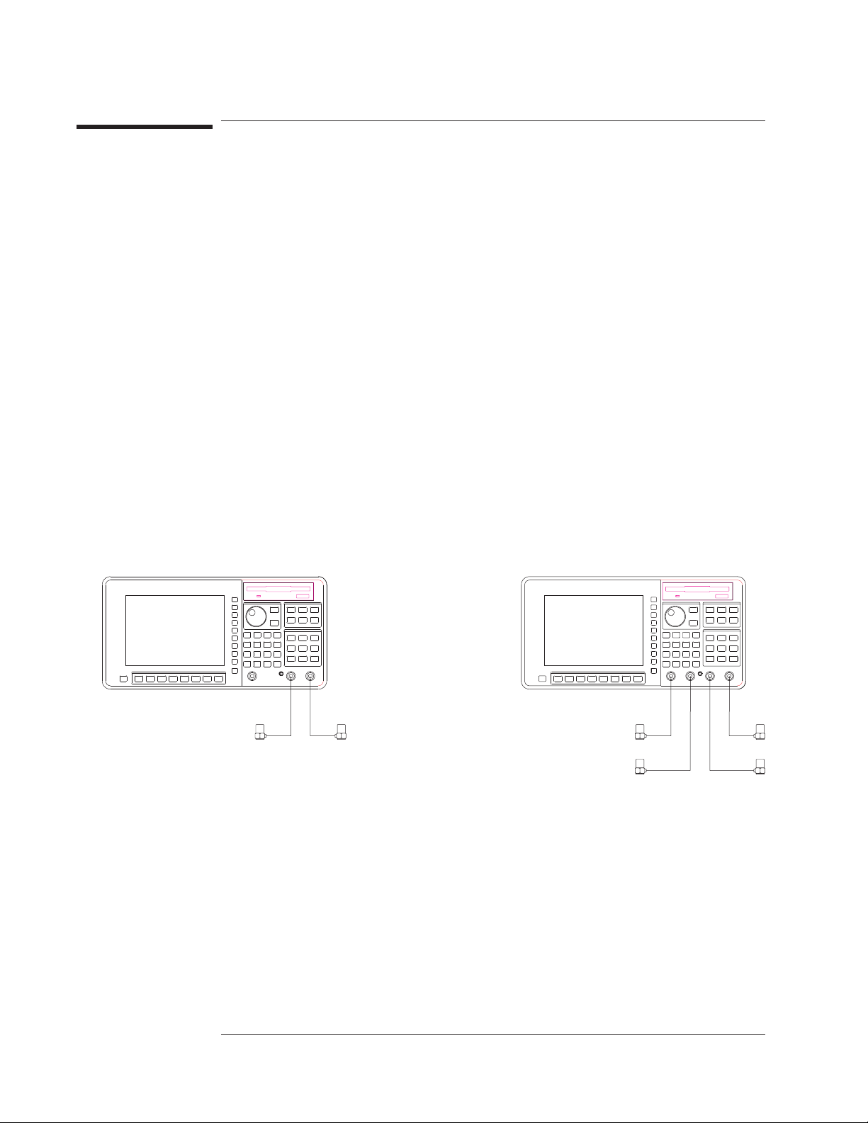
3 Connect the transducer output cables to the analyzer’s input channels, as shown in the

illustration.

You may also want to ac-couple an input channel if the corresponding transducer produces a significant amount of dc offset. Selecting ac-coupling prevents the dc overloads that can occur as you increase the channel’s sensitivity. You can select ac-coupling by pressing [ [

FRONT END CH* SETUP

COUPLING AC DC

]—to highlight AC. (The analyzer does this automatically

when you turn on a channel’s ICP power supply.)

If you preset the analyzer all ICP power supplies will be turned off and all channels will be set to dc-coupling. As a result, you may need to repeat some parts of this task after a preset.

]—located under

Option AY6

1-2

Page 45

Agilent 35670A Operator's Guide Measuring Rotating Machinery

To specify a transducer’s unit and sensitivity

1 Connect your transducers as described in the preceding task. 2 Press [

], then press [

Input

CHANNEL 1 2

] (or [

CHANNEL 1 2 3 4

]) to highlight the channel

connected to the transducer.

3 Press [

XDCR UNIT CHx SETUP][XDCR UNIT LABEL

[

MORE CHOICES

] to display additional units.)

]. (You can also press

4 If one of the displayed menus includes your transducer’s input unit, press the

corresponding softkey.

If neither menu includes your transducer’s input unit, you can enter the unit yourself (from the [ [

CLEAR ENTRY

5 Press [

MORE CHOICES

], then type a label and press [

][

Input

XDCR UNIT CHx SETUP][XDCR SENSITVTY

] menu): press [

USER LABEL][USER UNIT LABEL

ENTER

] <number> <unit>.

]

6 If you want the new unit and sensitivity factored into displayed amplitudes, press

[

XDCR UNIT ON OFF

The Agilent 35670A allows you to measure mechanical devices with a transducer. The transducer must produce an output voltage that’s proportional to some input energy over the range of frequencies measured. The unit you specify in this task is the one that’s used to quantify the input energy. The sensitivity you enter is the nominal sensitivity (or calibration factor) of the transducer. The unit and sensitivity settings are not lost when you preset or turn off the analyzer. Their use is disabled, however, because [

XDCR UNIT ON OFF

] to highlight ON.

] is set to OFF.

There is an advantage to directly selecting your transducer’s input unit instead of entering a user unit label in step 3. If you select one of the acceleration, velocity, or displacement units, you will be able to quickly convert displayed amplitudes from one of these units to another. For more information, see “To convert a displayed transducer unit” in chapter 11.

You can enter transducer sensitivity in V/EU, EU/V, or dB referenced to 1 V/EU. (EU is an abbreviation for engineering units—an alternate name for transducer units.) If you have a calibrator available, you may prefer to calibrate your transducers instead of entering their nominal sensitivities. The next task shows you how to calibrate a transducer.

1-3

Page 46

Agilent 35670A

Measuring Rotating Machinery Operator's Guide

To calibrate a transducer

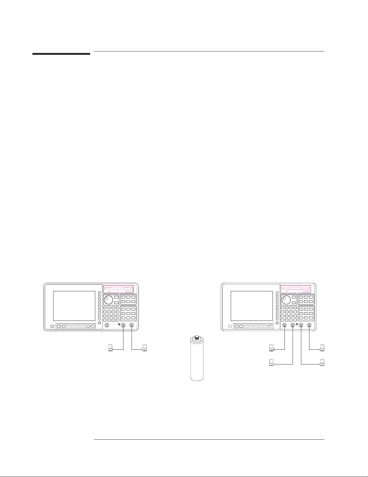
This task uses a calibrator, the FFT instrument mode, and the [

CAL VALUE AT MARKER

calibrator, you should enter the nominal transducer sensitivity as described in the previous task.

1 Initialize the analyzer.

Press [ Press [ Press [ want activated. Press [ channel whose transducer you will calibrate. Press [

][

Preset Inst Mode

CHANNELS 1 2

Meas Data

PWR SPEC CHANNEL x

DO PRESET

][

], then press [

2 Match the active trace’s display unit to the calibrator’s output unit.

Press [ whose transducer you will calibrate. Press [ corresponding to your calibrator’s output unit. (Additional units are displayed when you press [ Press [ Press [ Press [ calibrator’s output amplitude is specified as a peak value, PP if it is specified as a peak-to-peak value, or RMS if it is specified as a root-mean-square value.

], then press [

Input

XDCR UNIT CHx SETUP][XDCR UNIT LABEL

MORE CHOICES

][

Input Trace Coord

AMPLITUDE PK PP RMS

XDCR UNIT CHx SETUP

] softkey to calibrate a transducer. If you don’t have a

FFT ANALYSIS

] (or [

CHANNELS 1 2 4

CHANNEL 1 2

]) to highlight the number of channels you

](or[

CHANNEL 1 2 3 4

CHANNEL 1 2

] (or [

CHANNEL 1 2 3 4

]) to highlight the channel

], then press the softkey

].)

][

Y UNITS][EU

], then press [

XDCR UNIT ON OFF

] to highlight one of the following: PK if your

]) to highlight the

] to highlight ON.

1-4

Option AY6

Page 47

Agilent 35670A Operator's Guide Measuring Rotating Machinery

3 Connect the transducer’s output cable to the analyzer as described at the beginning of

this chapter, then secure the transducer to the calibrator.

4 Specify the measurement parameters.

Press [ frequency span. Press [

][

Freq

Window

], then press the down-arrow key if you want to reduce the

SPAN

][

FLAT TOP

] to maximize amplitude accuracy.

5 Press [ 6 Turn on the calibrator, then press [

], then press [

Scale

AUTOSCALE ON OFF

Start

] to highlight ON.

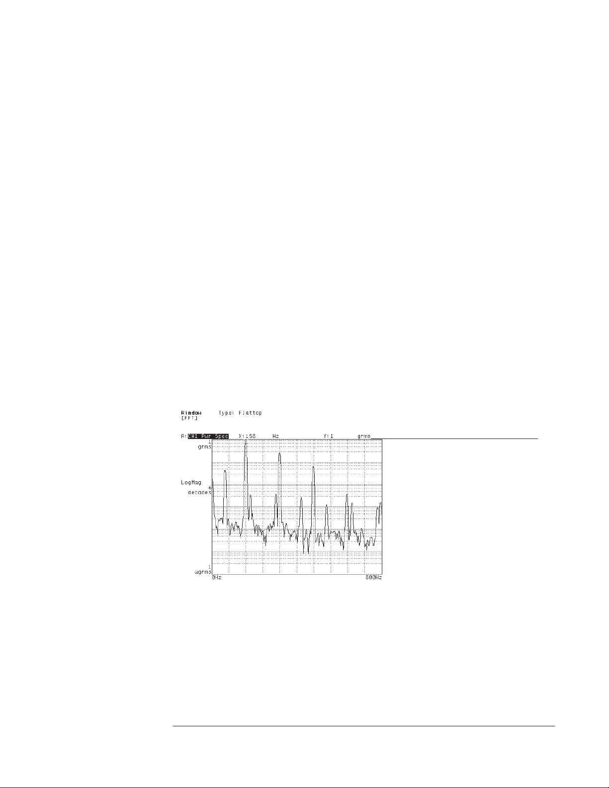
7 After the display has been updated at least once, move the marker to the calibrator’s

output frequency and enter calibrator’s output amplitude. Press [

Press [

Marker Input

][

MARKER TO PEAK

][

XDCR UNIT CHx SETUP][CAL VALUE AT MARKER

calibrator’s specified output amplitude and press [

The analyzer uses the number you enter in [ value for [

XDCR SENSITVTY

accuracy of your transducer measurements. The analyzer automatically stores this value and the [

XDCR UNIT LABEL

lost at preset or power-down. However, the values will be used only when [

XDCR UNIT ON OFF

] is set to ON.

], then type the

ENTER

CAL VALUE AT MKR

] to calculate a new

]. This new value is the calibration factor that ensures the

] value in nonvolatile memory, so they will not be

Y-axis readout matches calibration amplitude after you complete this task.

1-5

Page 48

Agilent 35670A

Measuring Rotating Machinery Operator's Guide

To measure vibration power

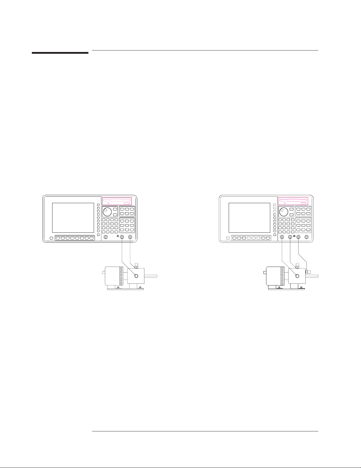
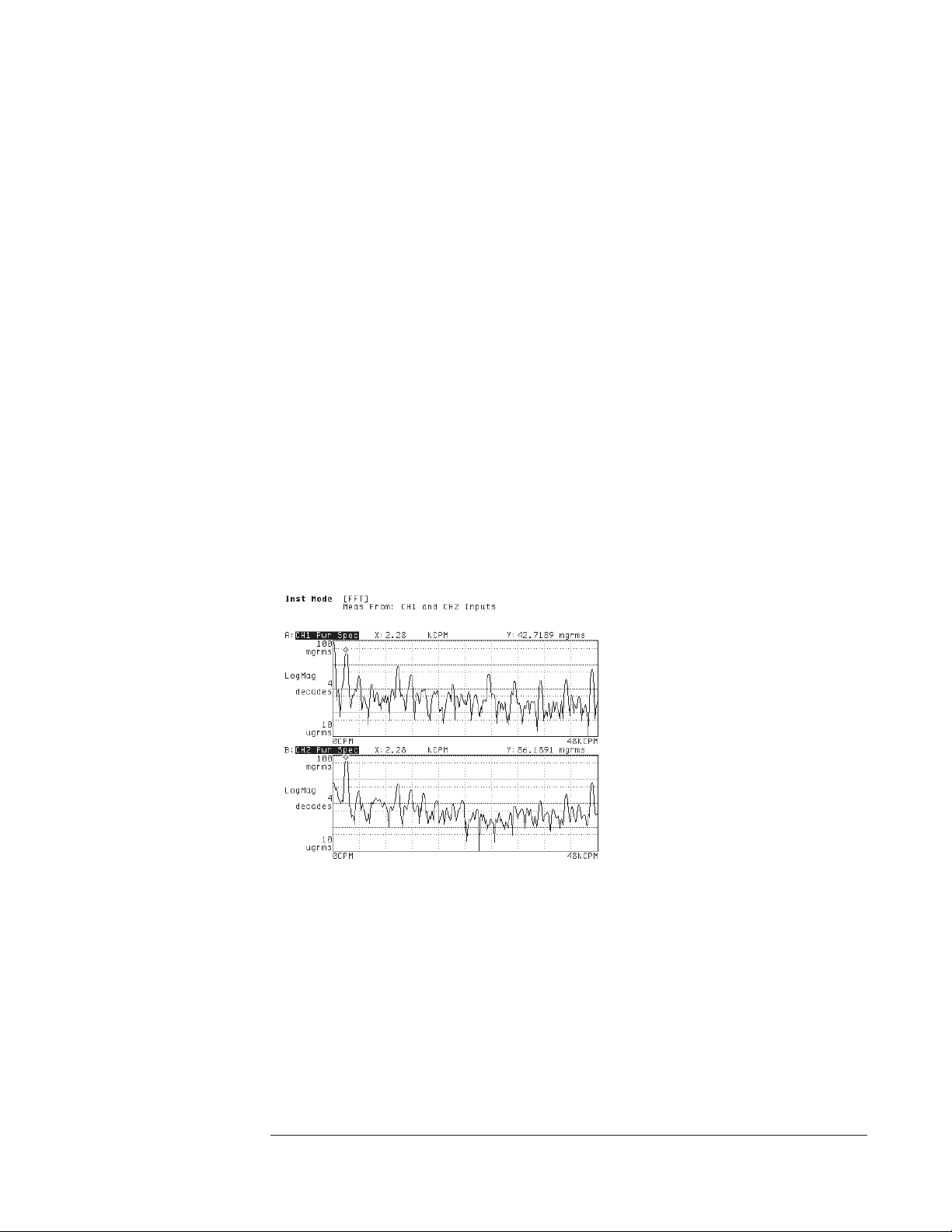
This task shows you how to use your calibrated transducers to measure vibration power. Although many vibration measurements are made using the order instrument mode, this task uses the FFT mode so you will not need to provide a tachometer signal. (All order-mode measurements require a tachometer signal.)

1 Initialize the analyzer.

Complete the preceding task, “To calibrate a transducer.” Press [

Active Trace

you are measuring with two, or [ Press [

Meas Data

outputtoeachtrace.

2 Secure each calibrated transducer to the device-under-test (DUT).

], then press [A] if you are measuring with one transducer, [AB]if

ABCD

][

ALL CHANNELS][PWR SPEC CHANNEL *

] if you are measuring with three or four.

] to assign one transducer’s

Option AY6

1-6

Page 49

Agilent 35670A Operator's Guide Measuring Rotating Machinery

3 Specify the measurement parameters.

Press [ the range of frequencies you want to measure. Press [

Freq

Input

][

] <number> <unit>, then press [

START

ALL CHANNELS][CH* AUTO UP ONLY

] <number> <unit> to select

STOP

4 Configure the display.

If you prefer to display frequency values in CPM rather than Hz, press [ [

X UNITS][CPM (SEC)

Press [

], then press [

Scale

AUTOSCALE ON OFF

] to highlight ON.

Trace Coord

]

5 Turn on the DUT, then press [

Start

The analyzer also allows you to display successive spectra in a map (or waterfall). To do this, complete the following steps: Activate the traces you want to view as a map. Press [ Press [

], then press [

Scale Disp Format

AUTOSCALE ON OFF

][

WATERFALL SETUP

] to highlight OFF.

], then press [

WATERFALL ON OFF

]to

highlight ON.

For more information on controlling and analyzing waterfall displays, see chapter 9, “Formatting the Display.”

1-7

Page 50

Agilent 35670A

Measuring Rotating Machinery Operator's Guide

To characterize a tachometer signal

Many rotating machinery measurements are only possible if you supply a tachometer signal. This task helps you characterize a tachometer signal so you can properly set up the parameters for the analyzer’s TACH connector.

1 Initialize the analyzer.

Press [ Press [ Press [

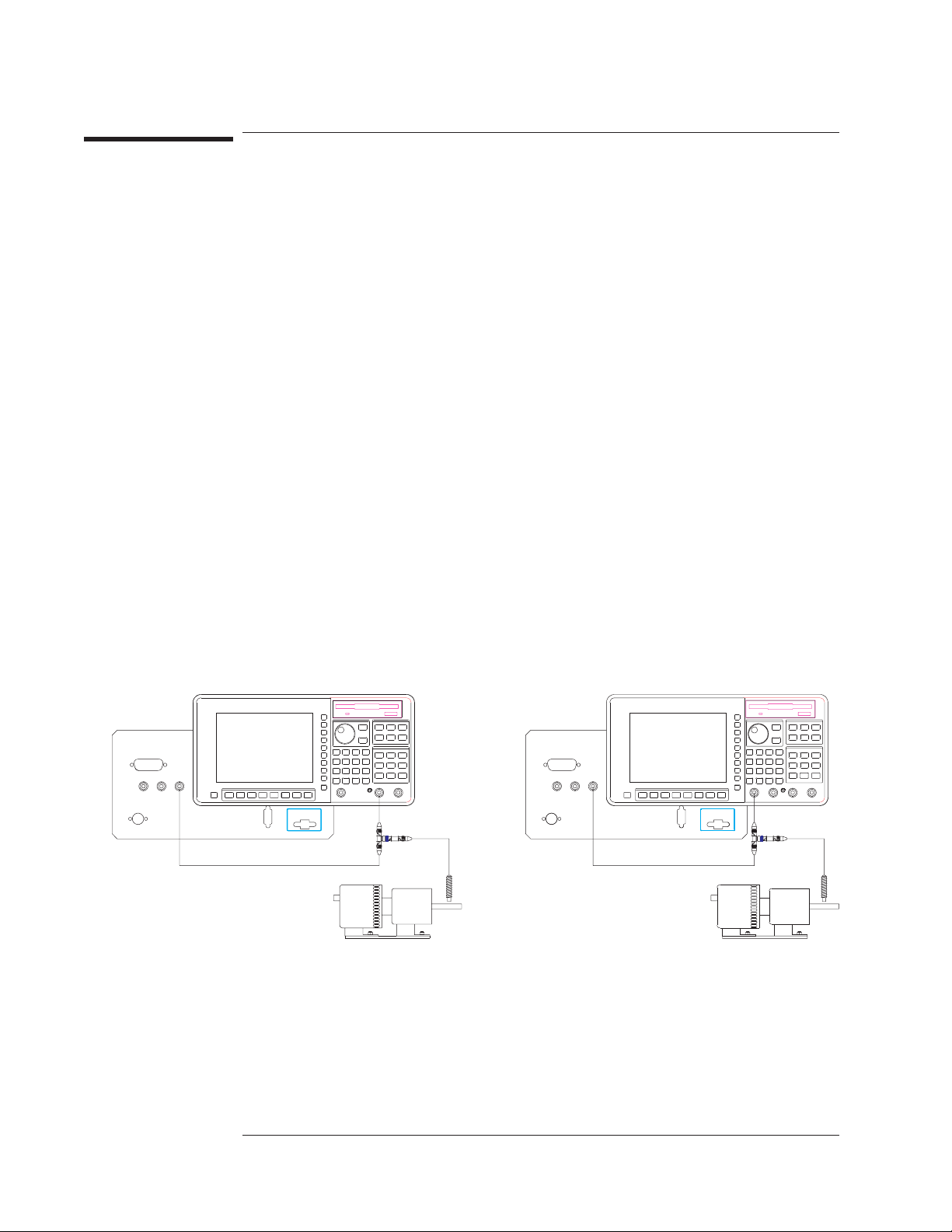
2 Connect the tachometer signal to the CH 1 connector on the analyzer’s front panel, and

to the TACH connector on its rear panel.

][

Preset Inst Mode Meas Data

DO PRESET

][

HISTOGRAM/TIME

][

UNFILTERD TIME CH 1

3 Press [

], then press [

Scale

AUTOSCALE ON OFF

] to highlight ON.

4 Specify the measurement parameters.

Press [ Press the up-arrow hardkey until there are several tachometer pulses on the display. Press [

][

Freq

Pause-Cont

RECORD LENGTH

] to pause the measurement.

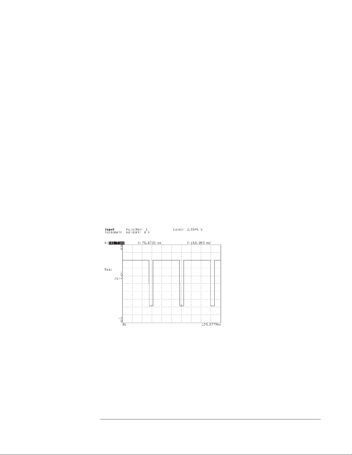
5 Use the marker to measure waveform amplitudes.

Press [

Marker

then turn the knob to place it on the low point. Note each point’s Y-axis readout (for use in the next step).

][

MARKER TO PEAK

] to place the marker on the waveform’s high point,

Option AY6

1-8

Page 51

Agilent 35670A Operator's Guide Measuring Rotating Machinery

6 Specify the tachometer parameters.

Press [ If the waveform’s high or low points fall outside a +/- 4 V range, press [

TRG RANGE +/- 20 4

Press [ detect the tachometer signal. If you want the analyzer to detect the falling (negative) edge of the waveform, press [

SLOPE POS NEG

Press [ pulses produced for each revolution of the device-under-test (DUT).

Input

][

TACHOMETR SETUP

] to highlight 20.

] <number> <unit> to specify the level at which you want the analyzer to

LEVEL

] to highlight NEG.

TACH PULS PER REV

] <number> [

] to specify the number of tachometer

ENTER

7 Verify the tachometer setup.

Press [

TACHDATAONOFF

Check to be sure that the tachometer readout—located at the top of the display— is stable.

You should specify a level and slope at which the tachometer signal is fairly “clean”—that is, a given pulse of the signal should pass through the specified level in the specified direction only once. If this is not possible, you can use [ to force the analyzer to ignore multiple passes through the same level. Enter a value that is just long enough to ensure that the analyzer ignores multiple passes through the same trigger level on a given pulse of the tachometer signal.

] to highlight ON.

HOLDOFF TIME

]

1-9

Page 52

Agilent 35670A

Measuring Rotating Machinery Operator's Guide

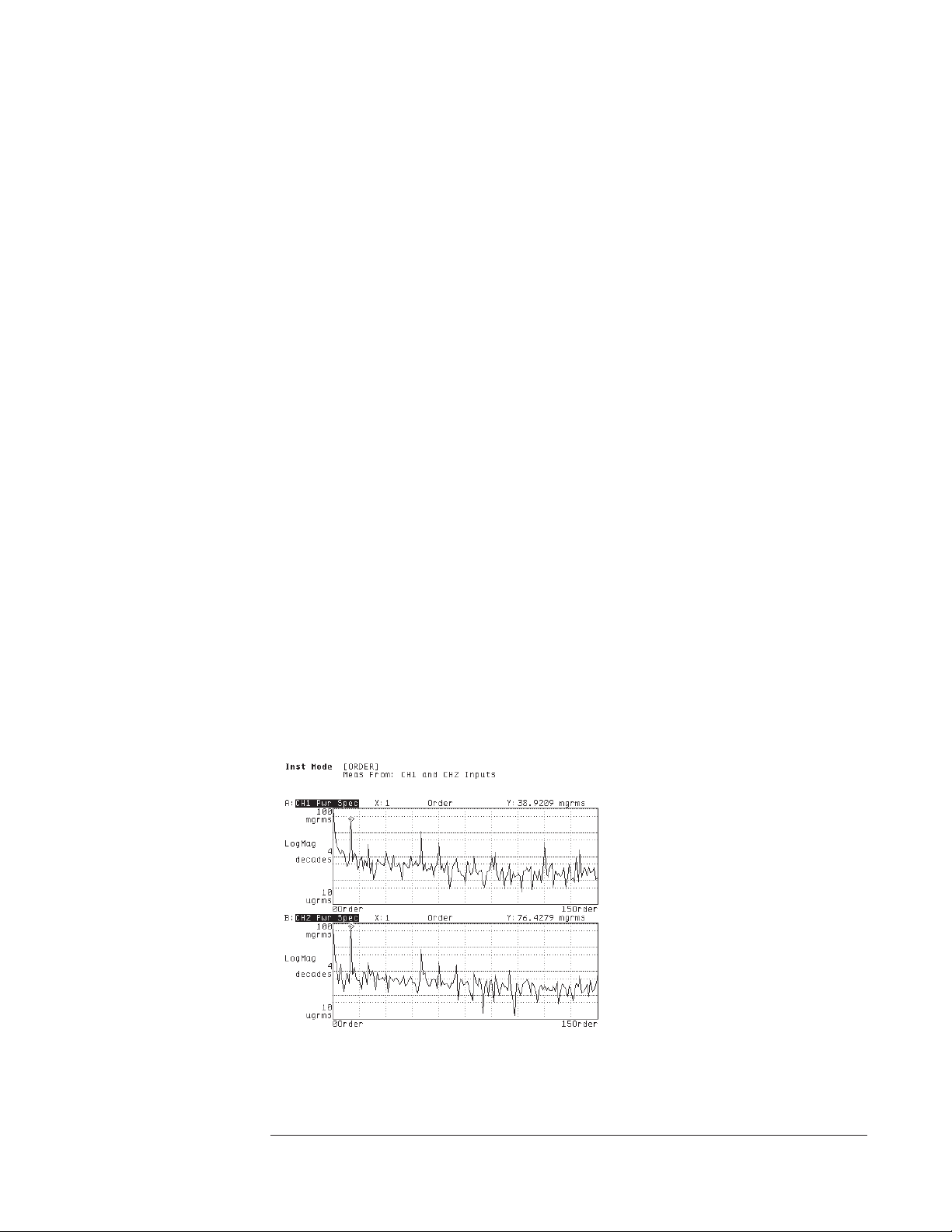
To measure an order spectrum

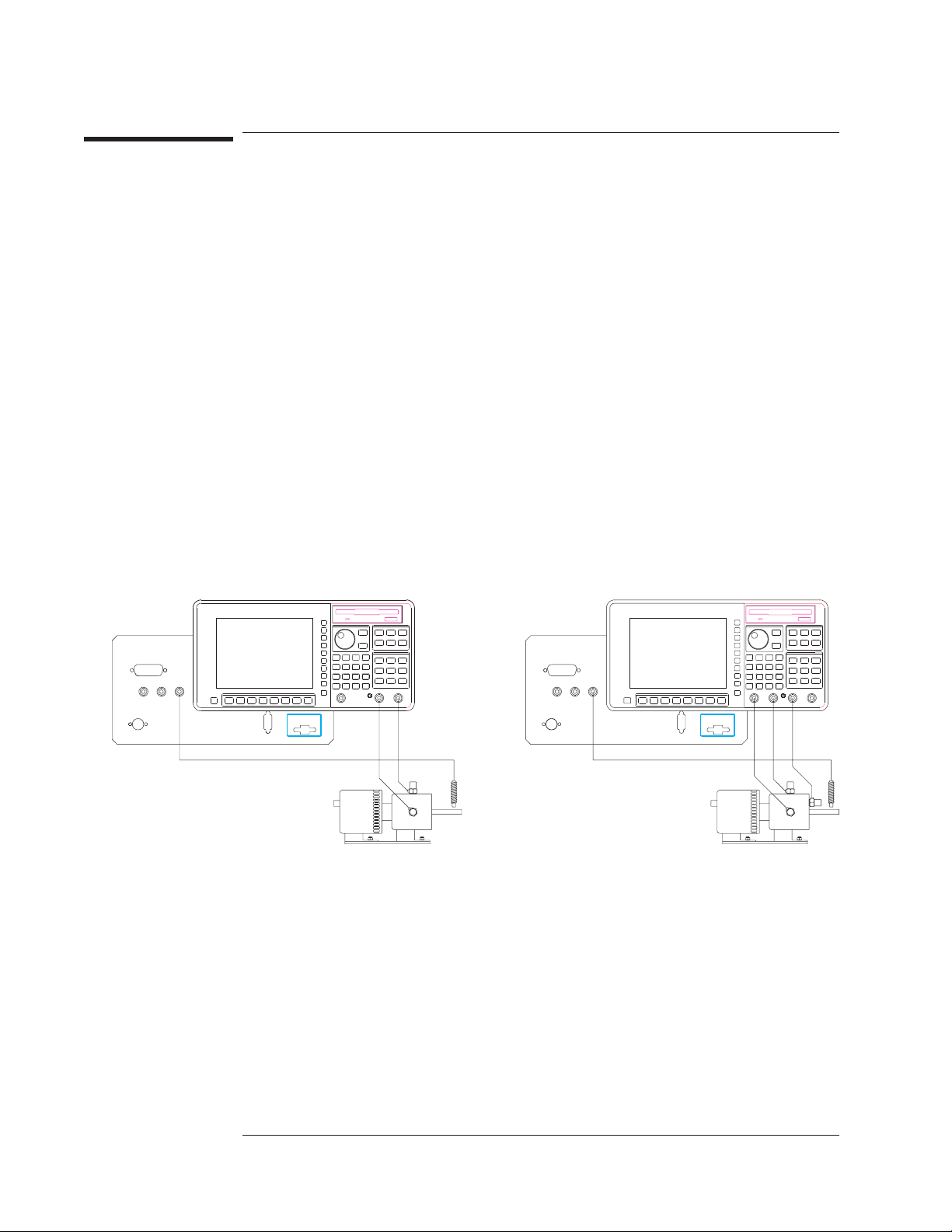
This task shows you how to use calibrated transducers to measure order spectra. Order-mode measurements are possible only if your analyzer is equipped with Option 1D0.

1 Initialize the analyzer.

Press [ Set up your tachometer parameters, as described in “To characterize a tachometer signal, ” but ignore that task’s instruction to preset the analyzer. Calibrate your transducers, as described in “To calibrate a transducer,” but ignore that task’s instruction to preset the analyzer. Press [ Press [ want activated. Press [ you are measuring with two, or [ Press [

2 Secure each calibrated transducer to the device-under-test (DUT).

][

Preset

Inst Mode

CHANNELS 1 2

Active Trace

Meas Data

DO PRESET

][

ORDER ANALYSIS

][

] (or [

CHANNELS 1 2 4

]) to highlight the number of channels you

], then press [A] if you are measuring with one transducer, [AB]if

ABCD

ALL CHANNELS][PWR SPEC CHANNEL *

] if you are measuring with three or four.

Option AY6

1-10

Page 53

Agilent 35670A Operator's Guide Measuring Rotating Machinery

3 Specify the measurement parameters.

Press [ orders you want to measure. Press [ the range of frequencies over which you will measure. Press [ Press [ For each active channel, press [ channel number, then press [

][

Freq

MIN RPM

DELTA ORDER

Input

MAX ORDER

] <number> [

RPM

] <number> [

CHANNEL 1 2

CHANNEL x RANGE

ORDERS

], then press [

ORDERS

] to specify the resolution of your X-axis.

] (or [

] to specify the maximum number of

MAX RPM

] <number> [

CHANNEL 1 2 3 4

]) to highlight its

]tospecify

RPM

] <number> <unit>.

4 Press [

], then press [

Scale

AUTOSCALE ON OFF

] to highlight OFF and press it again to

highlight ON.

5 Turn on the DUT, then press [

Start

Input channels do not autorange when an order mode measurement is running. As a result, you must set ranges carefully to ensure that they are not exceeded during the measurement. You can use one of the following methods:

• Manually set each channel’s range to a value that slightly exceeds the maximum

signal level you anticipate. Step 3 tells you how to set the range manually.

• Pause the measurement, then select up-only autoranging for all channels while the

DUT is running. To do this, press [ [

ALL CHANNELS][CH* AUTO UP ONLY

may want to select [

CH* FIXED RANGE

Pause-Cont

], then press [

]. (After the channels have autoranged, you

] to prevent spurious signals from increasing

Input

]

the range setting.

If an input signal does exceed the range of the corresponding channel, an OVLD message is displayed at the bottom of all affected traces. You should select a higher range for the overloaded channel before you restart the measurement.

1-11

Page 54

Agilent 35670A

Measuring Rotating Machinery Operator's Guide

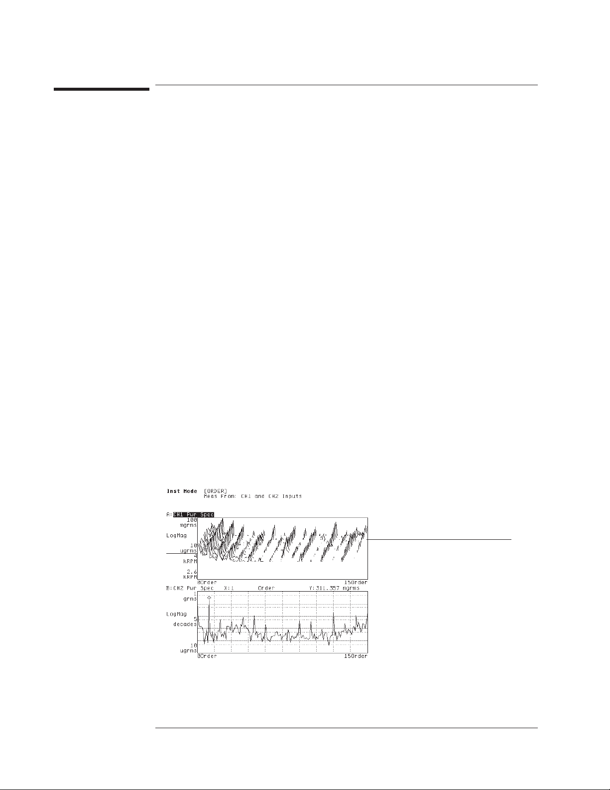
To display an rpm-stepped order map

1 Complete the task, “To measure an order spectrum.” 2 Press [ 3 Press [

Trigger

START RPM USAGE

runup measurement, or [

4 Press [

Rtn

][

ARM SETUP][RPM STEP ARM

], then press one of the following: [

RPM DECREASING

][

RPM STEP SIZE

]<number>[

RPM INCREASING

] for a rundown measurement.

] to specify how often the analyzer should

RPM

add a new measurement to the map.

5 Activate all traces you want to view as a map, then press [

Scale

][

AUTOSCALE ON OFF

to highlight OFF.

6 Press [

Disp Format

][

WATERFALL SETUP

], then press [

WATERFALL ON OFF

]to

highlight ON.

7 Turn on the device-under-test (DUT), then press [

If you select [

RPM INCREASING

frequency passes through the value of [ [

RPM DECREASING

], the first measurement is armed when the tachometer frequency passes through the value of [ [

MAX RPM

] are located under the [

Note: The analyzer measures at exact [ [

FREE RUN TRIGGER

] is selected under the [

], the first measurement is armed when the tachometer

MIN RPM

MAX RPM

] in a negative direction. [

] hardkey.

Freq

RPM STEP SIZE

Trigger

Start

] in a positive direction. If you select

MIN RPM

]and

] intervals only if

] hardkey.

For more information on controlling and analyzing waterfall displays, see chapter 9, “Formatting the Display.”

] for a

]

1-12

Waterfall skewing was turned on for this display.

Page 55

Agilent 35670A Operator's Guide Measuring Rotating Machinery

To display a time-stepped order map

1 Complete the task, “To measure an order spectrum.” 2 Press [ 3 Press [

Trigger

START RPM

][

ARM SETUP][TIME STEP ARM

] <number> [

] to specify tachometer frequency at which the first

RPM

measurement should be armed.

4 Press [

START RPM USAGE

want the first measurement to be armed above [ want it to be armed below [ armed as soon as you press the [

5 Press [

][

Rtn

TIME STEP SIZE

], then press one of the following: [

START RPM

Start

], or [

START RPM OFF

] hardkey.

START RPM

RPM INCREASING

], [

RPM DECREASING

] if you want it to be

]<number>[S] to specify how often the analyzer should

add a new measurement to the map.

6 Activate all traces you want to view as a map, then press [

Scale

][

AUTOSCALE ON OFF

to highlight OFF.

7 Press [

Disp Format

][

WATERFALL SETUP

], then press [

WATERFALL ON OFF

]to

highlight ON.

8 Turn on the device-under-test (DUT), then press [

Note: The analyzer measures at exact [ [

FREE RUN TRIGGER

] is selected under the [

TIME STEP SIZE

Trigger

Start

] intervals only if

] hardkey.

For more information on controlling and analyzing waterfall displays, see chapter 9, “Formatting the Display.”

]ifyou

]

1-13

Page 56

Agilent 35670A

Measuring Rotating Machinery Operator's Guide

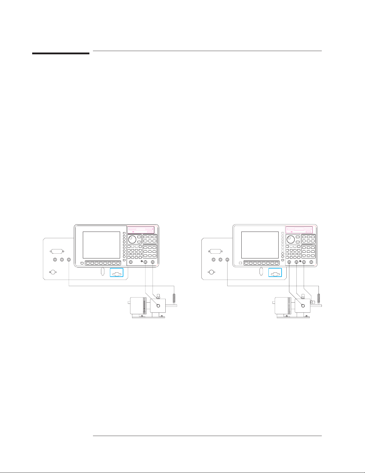
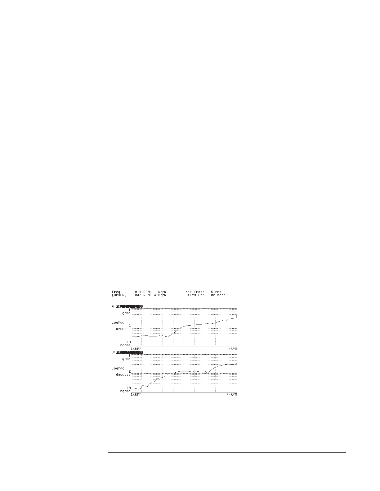
To measure an order track

This task shows you how to use calibrated transducers to measure order tracks. Before you complete this task, however, you may want to measure order spectra to help you identify the orders you want to track. Both of these order-mode measurements are possible only if your analyzer is equipped with Option 1D0.

1 Initialize the analyzer.

2 Secure each calibrated transducer to the device-under-test (DUT).

][

Preset

Inst Mode

CHANNELS 1 2

Freq

DO PRESET

][

ORDER ANALYSIS

], then press [

] (or [

CHANNELS 1 2 4

TRACK ON OFF

]) to highlight the number of channels you

] to highlight ON.

Option AY6

1-14

Page 57

Agilent 35670A Operator's Guide Measuring Rotating Machinery

3 Specify the measurement parameters.

Press [ to track. Press [ the range of frequencies over which you will measure. Press [ points in the track. Press [ you want to track. Press [ For each active channel, press [ channel number, then press [

][

Freq

MIN RPM

TRACK POINTS

TRACK SETUP

Input

MAX ORDER

] <number> [

], then press [

RPM

]<number>[

], then use the [

CHANNEL 1 2

CHANNEL x RANGE

ORDERS

ENTER

TRACK x ORDER

] to specify the highest order you want

MAX RPM

] <number> [

] to specify the number of measurement

] softkeys to specify which orders

] (or [

CHANNEL 1 2 3 4

] <number> <unit>.

]tospecify

RPM

]) to highlight its

4 Configure the display.

Press [

Active Trace

you are measuring with two, or [ Press [

Meas Data

press the [ Press [

TRACK x ORD n.nn

], then press [

Scale

], then press [A] if you are measuring with one transducer, [AB]if

ABCD

][

ALL CHANNELS][MORE CHOICES][ORDER TRK CHANNEL *

] if you are measuring with three or four.

], then

] softkey corresponding to the track you want to monitor.

AUTOSCALE ON OFF

] to highlight ON.

5 Turn on the DUT, then press [

Start

If you prefer to look at several tracks from a single channel (or at different tracks from different channels) activate each trace separately in step 4. Then, while a particular trace is activated, you can select the channel and track you want to display in that trace. Finally, you can press [

Disp Format

][

] to display all four traces at once.

QUAD

See “To measure an order spectrum” for additional information about setting ranges for your input channels.

1-15

Page 58

Agilent 35670A

Measuring Rotating Machinery Operator's Guide

To display an rpm-stepped order track

1 Complete the task, “To measure an order track.” 2 Press [ 3 Press [

Trigger

START RPM USAGE

runup measurement, or [

4 Press [

Rtn

][

ARM SETUP][RPM STEP ARM

], then press one of the following: [

RPM DECREASING

][

RPM STEP SIZE

]<number>[

RPM INCREASING

] for a rundown measurement.

] to specify how often the analyzer should

RPM

add a new point to the track.

5 Turn on the device-under-test (DUT), then press [

If you select [

RPM INCREASING

tachometer frequency passes through the value of [ you select [

RPM DECREASING

tachometer frequency passes through the value of [ [

MIN RPM

] and [

MAX RPM

Note: The analyzer measures at exact [ [

FREE RUN TRIGGER

] is selected under the [

], the first measurement point is armed when the

] are located under the [

RPM STEP SIZE

Trigger

Start

MIN RPM

MAX RPM

Freq

] in a positive direction. If

] hardkey.

] intervals only if

] hardkey.

] in a negative direction.

For more information on controlling and analyzing waterfall displays, see chapter 9, “Formatting the Display.”

] for a

1-16

Page 59

Agilent 35670A Operator's Guide Measuring Rotating Machinery

To display a time-stepped order track

1 Complete the task, “To measure an order track.” 2 Press [ 3 Press [

Trigger

START RPM

][

ARM SETUP][TIME STEP ARM

] <number> [

] to specify tachometer frequency at which the first

RPM

measurement point should be armed.

4 Press [

START RPM USAGE

want the first measurement point to be armed above [ if you want it to be armed below [ armed as soon as you press the [

5 Press [

][

Rtn

TIME STEP SIZE

], then press one of the following: [

START RPM

] hardkey.

Start

], or [

START RPM OFF

RPM INCREASING

], [

RPM DECREASING

] if you want it to be

]<number>[S] to specify how often the analyzer should

add a new point to the track.

6 Turn on the device-under-test (DUT), then press [

Note: The analyzer measures at exact [ [

FREE RUN TRIGGER

] is selected under the [

TIME STEP SIZE

Trigger

Start

] intervals only if

] hardkey.

For more information on controlling and analyzing waterfall displays, see chapter 9, “Formatting the Display.”

]ifyou

]

1-17

Page 60

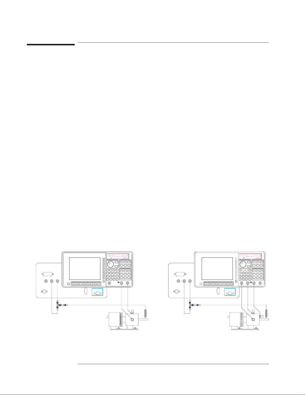
Agilent 35670A

Measuring Rotating Machinery Operator's Guide

To display phase relative to the tachometer signal

1 Complete one of the three preceding order track tasks. 2 Connect the tachometer signal to both the TACH and the EXT TRIG connectors. 3 Press [ 4 Press [

Trigger

TACHOMETR SETUP

][

EXTERNAL TRIGGER

], then note the settings of [

] and [

LEVEL

SLOPE POS NEG

use in the next step.

5 Press [

match the corresponding [

6 Press [

][

Rtn

TRIGGER SETUP

EXT RANGE +/- 10 2

], then set [

TACHOMETR SETUP

USER EXT LEVEL

]softkeys.

] and [

SLOPE POS NEG

]to

] to highlight 2 if the tachometer signal falls within a +/- 2 V

range, or 10 if it falls outside that range.

7 Activate the traces you will use to display phase, then press [ 8 Turn on the device-under-test (DUT), then press [

Start

Trace Coord

][

PHASE

When you set up an order track measurement as described in this task, the analyzer displays phase data for every channel relative to the tachometer signal. However, this setup provides useful phase information only if the tachometer signal provides one pulse per revolution of the DUT you are measuring.

When you select free run triggering, the analyzer displays phase data for each channel relative to its reference channel. For two-channel Agilent 35670As, channel 1 is the reference for both channels. For four-channel Agilent 35670As, channel 1 is the reference for all channels only when [

REF CHANS 1 1,3

]—located under the [

Inst Mode

hardkey—is set to 1. Channel 1 is the reference for 1 and 2, and channel 3 is the reference for 3 and 4 when [

REF CHANS 1 1,3

] is set to 1,3.

]for

]

1-18

Option AY6

Page 61

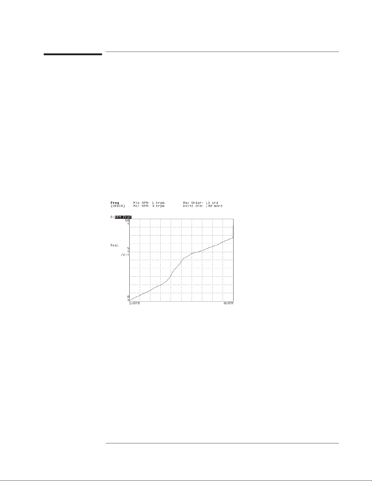
Agilent 35670A Operator's Guide Measuring Rotating Machinery

To display an rpm profile

1 Complete one of these tasks: “To measure an order spectrum” or “To measure an

order track.”

2 Press [ 3 Press [

Active Trace

Meas Data

], then press [A], [B], [C], or [D] to activate one of the traces.

][

MORE CHOICES][RPM PROFILE

An rpm profile allows you to monitor changes in the tachometer frequency. Each time the analyzer measures another order spectrum or adds another point to an order track, it also adds another point to the rpm profile. When you are measuring an order spectrum, the total number of points in the profile is equal to the value of [

WATERFALL STEPS

] (located under [

Disp Format

][

WATERFALL SETUP

]). When you are measuring an order track, the total number of points in the profile is equal to the value of [

TRACK POINTS

] (located under [

Freq

]).

1-19

Page 62

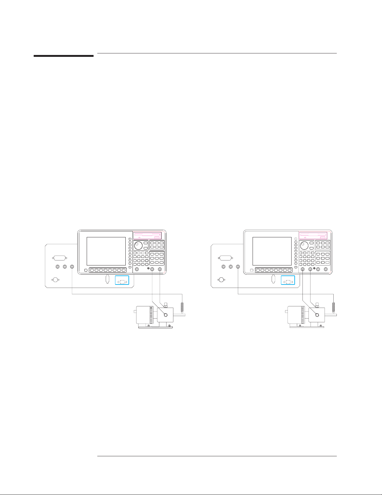
Agilent 35670A

Measuring Rotating Machinery Operator's Guide

To display an orbit diagram

If you mount two calibrated transducers at 90° to each other, you can use the analyzer to display an orbit diagram. This measurement is possible only if your analyzer is equipped with Option 1D0.

1 Connect the horizontal transducer to channel 1 and the vertical transducer to channel 2. 2 Initialize the analyzer.

][

Preset

Inst Mode

CHANNELS 1 2

Disp Format Meas Data

DO PRESET

][

ORDER ANALYSIS

][

] (or [

CHANNELS 1 2 4

SINGLE

ORBIT 2/1

]) to highlight 2. ]. ].

Option AY6

1-20

Page 63

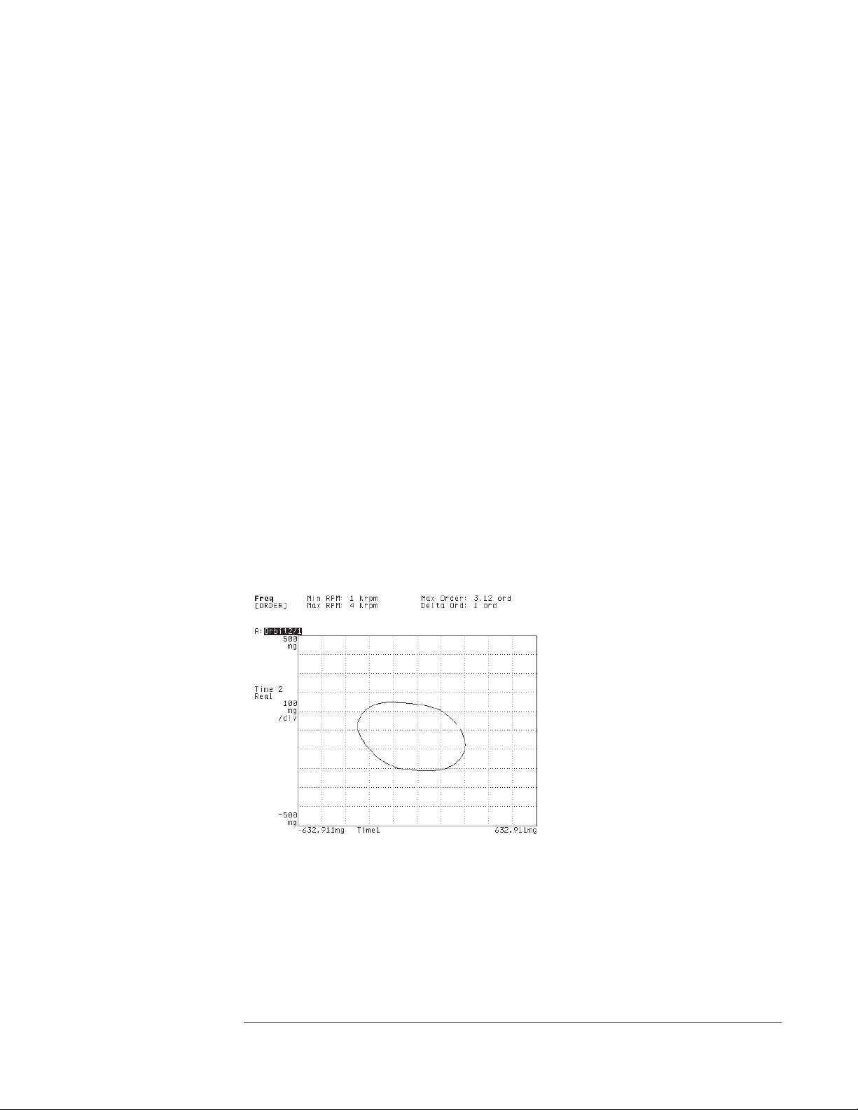
Agilent 35670A Operator's Guide Measuring Rotating Machinery

3 Specify the measurement parameters.

Press [ orders you want to measure. Press [ the range of frequencies over which you will measure. Press [ Press [ For both channels, press [ number, then press [

][

Freq

MIN RPM

DELTA ORDER

Input

MAX ORDER

] <number> [

], then press [

RPM

]1[

ORDERS

CHANNEL 1 2

CHANNEL x RANGE

ORDERS

] (or [

] to specify the maximum number of

MAX RPM

CHANNEL 1 2 3 4

] <number> <unit>.

] <number> [

]tospecify

RPM

]) to highlight its channel

4 Press [ 5 Turn on the device-under-test (DUT), then press [

], then press [

Scale

AUTOSCALE ON OFF

] to highlight ON.

Start

With a four-channel Agilent 35670A, you can use four transducers to display two independent orbit diagrams. This allows you to measure two points on the DUT simultaneously. Use channels 1 and 2 to measure one point, and channels 3 and 4 to measure the other (with the horizontal transducers connected to channels 1 and 3). You must modify the last few instructions in step 2, as shown below:

Press [

CHANNELS 1 2 4

] to highlight 4 (rather than 2), then press [

REF CHANS 1 1,3

highlight 1,3. Press [

Disp Format

][

UPPER/LOWER

Activate traces A and B, then press [ Activate trace B, then press [

Meas Data

CHANNEL 1 2 3 4

][

ALL CHANNELS][ORBITS */*

] to highlight 3.

]to

1-21

Page 64

1-22

Page 65

Measuring Structures

Page 66

Page 67

Measuring Structures

2-1

Page 68

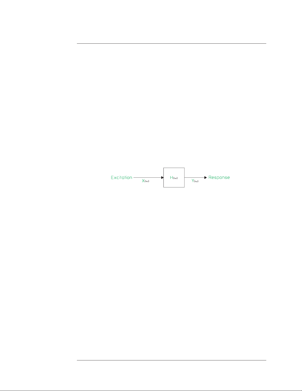
Figure 2-1.

Agilent 35670A

Measuring Structures Operator's Guide

Measuring Structures

All structures have natural frequencies of resonance. A type of modal testing known as the frequency response function measures the input excitation and output response simultaneously. See figure 2-1.

The method is based on an assumption that the system under-test is linear and stable.

System Block Diagram

This chapter introduces some of the Agilent 35670A’s measurement capability for measuring structures. Additional information is available in Agilent 35288,

DSA Concept Documentation or Agilent Technologies, Inc.’s application note,

AN243-3, Technologies, Inc. Sales/Service Office).

2-2

The Fundamentals of Modal Testing (available from your local Agilent

Page 69

Agilent 35670A Operator's Guide Measuring Structures

Setting Up Your Test

The basic test set-up required for making frequency response measurements depends upon the type of structure to be tested and the level of results desired. Other factors, including the support fixture and excitation method, affect the amount of hardware needed to perform the test. For making measurements on simple structures, the exciter mechanism can be as basic as an instrumented hammer and requires a minimum amount of hardware. An electrodynamic shaker may be needed to excite a more complicated structure.

The first step in setting up a structure for frequency response measurements is to consider the fixturing mechanisms. This is a key step in the process as it affects the overall structural characteristics. The selection of a fixture goes beyond the scope of this book. Several texts are available that focus on test fixtures. They include:

• Vibration and Shock Test Fixture Design by Wayne Tustin and Robert Mercado

(Tustin Technological Institute, 1984).

• L.D.MitchellandK.B.Elliott,“HowToDesignStingersforVibrationTestingof

Structures,” Sound and Vibration, April 1984.

• Modal Testing: Theory and Practice by Dave J. Ewins (Wiley Interscience, 1984).

The next step in the measurement process involves selecting an excitation function along with an excitation mechanism. The choice of the excitation function dictates the choice of the excitation mechanism. The choice depends on several factors:

• available signal processing equipment

• characteristics of the structure

• general measurement considerations

• the excitation mechanism.

The shaker test and the impact test are the most common excitation mechanisms.

Once an excitation mechanism has been setup to force the structure into motion, you need to select the transducers which sense the force and motion. The piezoelectric transducer is widely used. It is an electromechanical sensor which generates an electrical output when subjected to vibration.

2-3

Page 70

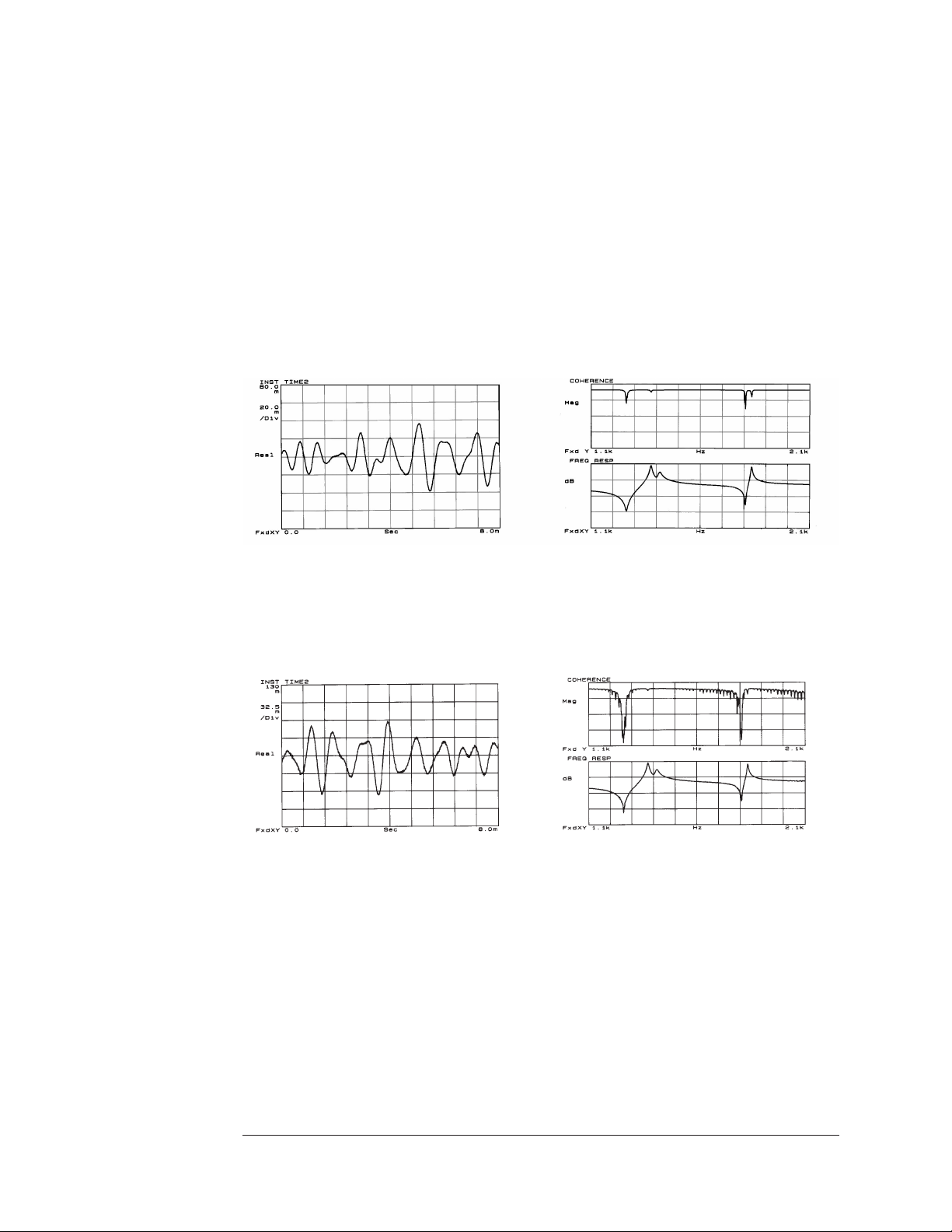
Figure 2-2.

Agilent 35670A

Measuring Structures Operator's Guide

Interpreting Measurement Results

To ensure high quality measurements, it is important to make some trial measurements and examine them before collecting data.

After setting up the structure, you should look at the time domain signals. The input range settings should be set at no more than two times the maximum signal level. This is known as half-ranging. See figure 2-2.

Figure 2-3.

InputHalfRanging

When the response input level is very low relative to the analyzer, noise appears between the peaks in the frequency response. This results in a poor coherence function. See figure 2-3. This is called under-ranging.

Input Under Ranging

2-4

Page 71

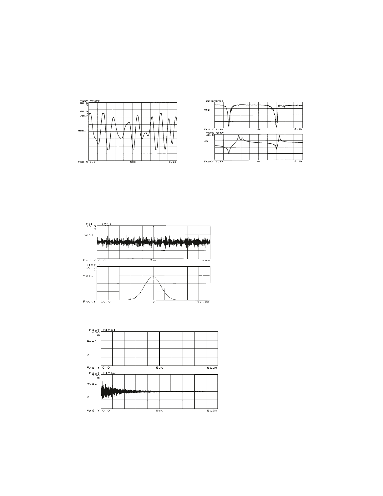
Figure 2-4

Agilent 35670A Operator's Guide Measuring Structures

When the response input level is severely overloading, the analyzer’s input is clipped. This results in a poor frequency response and poor coherence because the actual response is not being measured. This is called over-ranging. See figure 2-4.

Input Over Ranging

You should also verify that the signals are the type you expect. With a random signal, you should measure the histogram to verify that it has a Gaussian distribution. See figure 2-5. In addition, you can visually inspect transient signals. See figure 2-6.

Figure 2-5.

Figure 2-6.

Random Noise

Histogram

Verify Random Test Signals

Typical Force

Exponential Decaying

Responce

Verify Transient Test Signals

2-5

Page 72

Agilent 35670A

Measuring Structures Operator's Guide

Improving Accuracy

Averaging and windowing are measurement techniques that help to improve the accuracy of a measurement.

Averaging

Use measurement averaging to reduce the statistical variance of a measurement with a random excitation function. Averaging also reduces the effects of nonlinearities.

RMS averaging, which is also called “power” averaging, is calculated by squaring all the values, adding the squares together, dividing by the number of measurements (mean) and taking the square root of the result. RMS averaging is a good technique for determining the average power level. It does not improve the signal-to-noise ratio. RMS averaging only makes a more accurate estimate of the total signal plus noise power.

Linear averaging improves the signal-to-noise ratio of a measurement, but it can only be used if a trigger signal which is synchronous with the periodic part of the spectrum is available. (The periodic part of the input will always be exactly the same in each time record whereas the noise will vary.) Linear averaging is calculated by adding together a series of synchronized triggered measurements and dividing by the number of records. The noise is different in each time record and will tend to average to zero.

2-6

Page 73

Agilent 35670A Operator's Guide Measuring Structures

Windowing

Use a windowing function to reduce leakage if your signal is not periodic within the time record. (Leakage is the effect of smearing or leaking energy into adjacent frequency lines which results in distorting the spectra.) The effect of leakage underestimates the amplitude of the spectra and overestimates the damping factor.

A windowing function artificially forces the signal to 0 at the beginning and at the end of the time record. The signal then appears to be periodic. A windowing function does not eliminate leakage completely and may distort the results by eliminating some of the data. If possible, another technique is to use a signal that is periodic within the time record, such as burst random or periodic chirp. Such signals eliminate the leakage problem.

2-7

Page 74

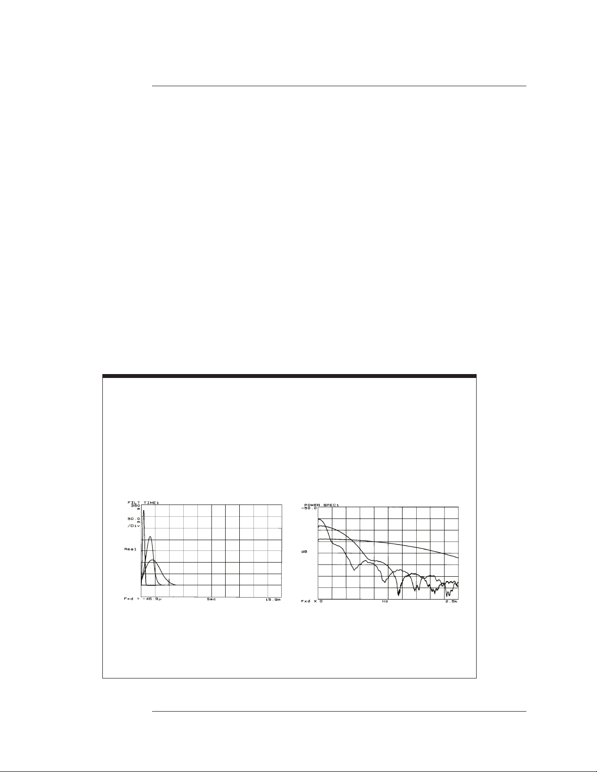
Agilent 35670A

Measuring Structures Operator's Guide

Impact Testing

To find natural frequencies, an impulse response measurement can be performed on the structure and the Agilent 35670A can be used to compute the frequency response of the structure. An instrumented hammer impacts the structure and an accelerometer measures the response.

The impact hammer has a load cell that measures the level of force during the impact. In a modal test, impact measurements are made at various places on the structure. The resulting frequency functions can be stored for later analysis by a modal software package.

Impact testing is convenient because it provides shorter measurement times and requires little hardware. However, it can be difficult to implement the test and to produce consistent results. It is difficult to control the velocity of the hammer, so the force level is usually controlled by varying the mass of the hammer. Another disadvantage is that the force spectrum of an impact test cannot be band-limited at lower frequencies when making zoom measurements (starting frequency > 0 Hz) so lower out-of-band modes will be excited.

Choosing a Tip For the Hammer

The frequency content of the energy applied to the structure is a function of the stiffness of the contacting surfaces and the mass of the hammer. It is not feasible to change the stiffness of the test object, therefore, the frequency content is controlled by varying the stiffness of the hammer tip.

Hard

Medium

Soft

Pulse

The harder the tip the shorter the pulse duration resulting in a higher frequency content.

A rule of thumb is to choose a tip so that the amplitude of the force spectrum is no more than 10 dB to 20 dB down at the maximum frequency of interest.

Soft

Medium

Hard

2-8

Page 75

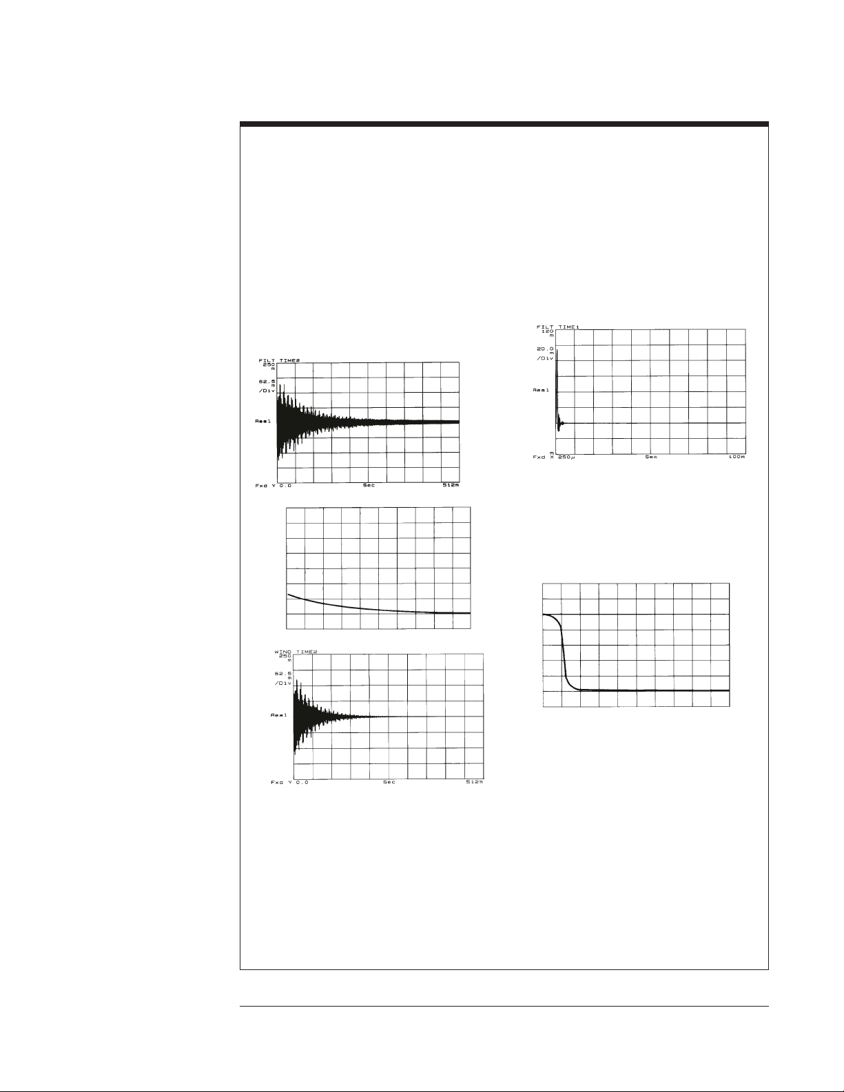
Agilent 35670A Operator's Guide Measuring Structures

Compensating For Noise and Leakage

Noise can be present in either the force or response signal as a result of a long time record. Leakage can be present in the response signal as a result of a short time record.

Noise may appear after the force pulse. The force window eliminates any noise without affecting the pulse itself.

The response signal is an exponentially decaying function. If the structure is heavily damped, the response may decay out before the end of the time record.

Responce

Exponential Window

Noise may be present in the remaining part of the time record. If the structure is lightly damped, the response may continue beyond the end of the time record. The effect is leakage.

The exponential window minimizes leakage and can eliminate any remaining noise in the time record. The exponential window uses a time constant which is the time required for the amplitude to be reduced by a factor of 1/e. A rule of thumb for setting the time constant is approximately 1/4 the time record length, T.

Force Pulse

Windowed Responce

Force Window

2-9

Page 76

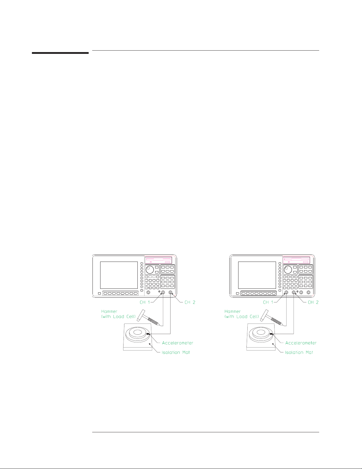
Agilent 35670A

Measuring Structures Operator's Guide

To measure a driving point measurement

A driving point measurement places the response accelerometer at the point where the impact hammer hits the device.

1 Initialize the analyzer.

Press [ Press [ Press [

2 Connect the device-under-test (DUT) as shown in the illustration below. 3 Specify the measurement parameters.

Press [ Press [ Press [ Press [ Press [ Press [ Press [ Press [ Press [ Press [ Press [ Press [

][

Preset Active Trace Meas Data

Freq Input

CHANNEL 1 2 3 4 CHANNEL 1 RANGE CHANNEL 1 2 3 4

CHANNEL 2 RANGE

Window

FORC EXPO SETUP CHANNEL 1 FORC EXPO FORCE WIDTH CHANNEL 2 FORC EXPO EXPO DECAY

DO PRESET

][

START

][

FORCE EXPO

][AB].

FREQ RESP 2/1

] <number> <unit>, then press [

] to highlight 1.

] <number> <unit>.

] to highlight 2.

] <number> <unit>.

] to highlight FORC.

] to highlight EXPO.

] <number> <unit>.

STOP

2-10

Page 77

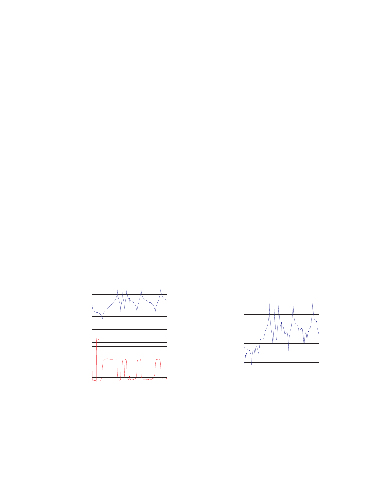
Agilent 35670A Operator's Guide Measuring Structures

4 Specify the triggering and averaging parameters.

Press [

Trigger

Press [

TRIGGER SETUP][CHANNEL LEVEL

or Press <number> <unit>. Press [

CHANNEL 1 DELAY

Press [

CHANNEL 1 2 3 4

Press [

CHANNEL 2 DELAY

Press [

Avg

][

CHANNEL 1 2 3 4

], then press [

] to highlight 1.

][

] <number> <unit>.

+/-

] to highlight 2.

][

] <number> <unit>.

+/-

AVERAGE ON OFF

]<number>[

PERCENT %

] to highlight ON.

]

5 Configure the display.

Press [ Press [ Press [ Press [ Press [

Trace Coord Active Trace Trace Coord Active Trace

], then press[

Scale

][

X-AXIS LIN LOG

][B]. ][

PHASE

][AB].

AUTOSCALE ON OFF

] to highlight LIN.

] to highlight ON.

6 Measure the DUT.

Press [ Slowly tap the device 10 times with the impact hammer at or near the accelerometer.

Start

If your hammer taps consistently result in overloads, increase the input ranges in step 3 until overloads no longer occur.

Specifying a trigger delay in step 4 allows you to see the leading edge of the hammer tap.

Trac Coord

A: dBMag B: Phase

[FFT]

C: Real D: Real

A: Freq Resp2/1 X:0 Hz Y:2.58684dB

dBMag

/div

-50

0Hz 3.2kHzAVG: 10

B: Freq Resp2/1

Phase

X:0 Hz Y:-180 deg

180

deg

/div

-180

deg

0Hz 3.2kHzAVG: 10

Avg

Type:RMS Number:10

[FFT]

UpdateRt: 5 Overlap:0%

A: Freq Resp2/1 X:0 Hz Y:-20.464dB

dBMag

/div

-40

0Hz 3.2kHzAVG: 10OVLD

Overload causes distortion in the frequency response.

Indicates an overload is included in the average measurement.

2-11

Page 78

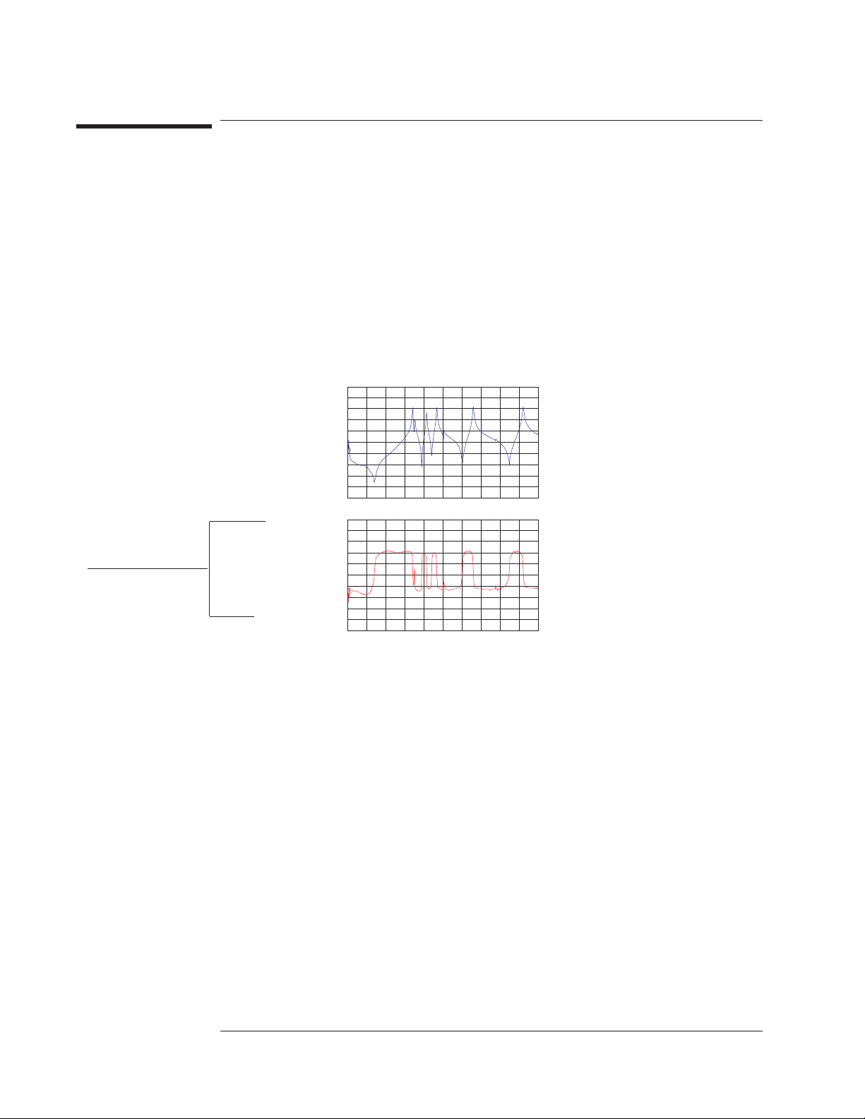
Agilent 35670A

Measuring Structures Operator's Guide

To view unwrapped phase of a driving point measurement

1 Measure a driving point measurement.

Values indicate unwrapped phase.

2 Press [

Press [

3 Press [

Active Trace Trace Coord

][

Scale

AUTOSCALE ON OFF

Trac Coord

[FFT]

A: Freq Resp2/1 X:0 Hz Y:3.49835dB

dBMag

B: F reqRe sp2/1

Phase

][B]. ][

UNWRAPPED PHASE

A: dB Mag B: Phase

C: Real D: Real

/div

-40

0Hz 3.2kHzAVG: 10

X:0 Hz Y:-180 deg

150

deg

/div

-350

deg

0Hz 3.2kHzAVG: 10

] to highlight ON.

2-12

Page 79

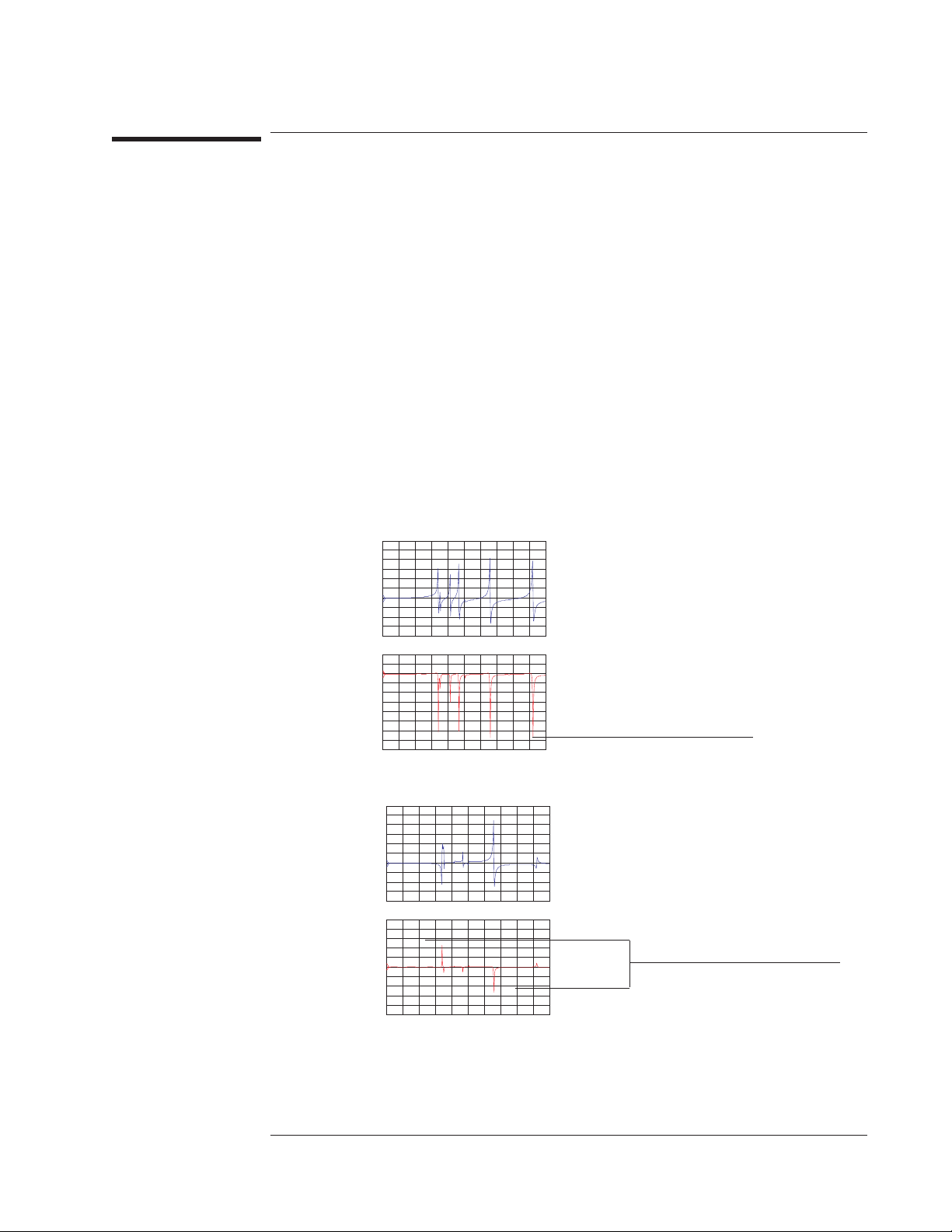
Agilent 35670A Operator's Guide Measuring Structures

To view the real and imaginary components of a driving point measurement

1 Measure a driving point measurement. 2 Press [

Press [

3 Press [

Press [

4 Press [

Press [

Active Trace Trace Coord

Active Trace

IMAGINARY PART

Active Trace

][

Scale

][A]. ][

MORE CHOICES][REAL PART

][B].

][AB].

AUTOSCALE ON OFF

] to highlight ON.

A characteristic of a driving point measurement is that the imaginary components all point in the same direction. When the imaginary components do not all point in the same direction, it usually indicates that the accelerometer and the impact point for the hammer were separated. In addition, the relative frequencies are the same, but the relative amplitudes at each resonance are different.

Trac Coord

A: Real B: Ima g

[FFT]

C: Real D: Real

A: FreqResp2/1 X:0 Hz Y:-1.496

120

Real

/div

-80

0Hz 3.2kHzAVG: 10

B: Freq Resp2/ 1

Imag

Trac Coord

[FFT]

A: FreqResp2/1 X:0 Hz Y:-1.2918

X:0 Hz Y:0

/div

-160

A: Real B: Ima g

C: Real D: Real

120

A characteristic of a driving point measurement is that all imaginary components point in the same direction.

Real

/div

-80

0Hz 3.2kHzAVG: 10

B: Freq Resp2/ 1

Imag

X:0 Hz Y:0

250

/div

-250

0Hz 3.2kHzAVG: 10

When the accelerometer and impact point are separated by 90o, the imaginary components do not point in the same direction.

2-13

Page 80

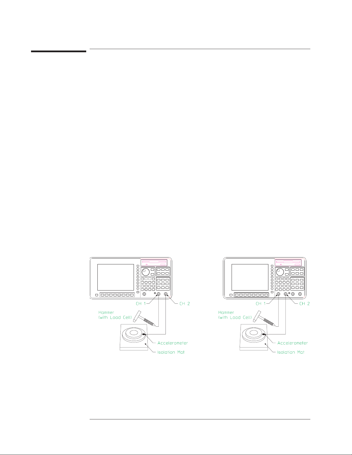
Agilent 35670A

Measuring Structures Operator's Guide

To preview the time record

The Agilent 35670A’s preview lets you examine each time record and decide whether or not to include the data in an averaged measurement. This task performs a driving point measurement with manual preview.

1 Initialize the analyzer.

Press [ Press [ Press [

2 Connect the device-under-test (DUT) as shown in the illustration below. 3 Specify the measurement parameters.

Press [ Press [ Press [ Press [ Press [ Press [ Press [ Press [ Press [ Press [ Press [ Press [

][

Preset Meas Data Active Trace

Meas Data

CHANNEL 1 2 3 4 TIME CHANNEL 1

Freq Input

CHANNEL 1 2 3 4 CH1 FIXED RANGE CHANNEL 1 2 3 4

CH2 FIXED RANGE

Window

FORC EXPO SETUP CHANNEL 1 FORC EXPO FORCE WIDTH CHANNEL 2 FORC EXPO EXPO DECAY

DO PRESET

][

START

][

FORCE EXPO

FREQ RESP 2/1

][B].

] to highlight 1.

] <number> <unit>, then press [

] to highlight 1.

] <number> <unit>.

] to highlight 2.

] <number> <unit>.

] to highlight FORC.

] to highlight EXPO.

] <number> <unit>.

STOP

2-14

Option AY6

Page 81

Agilent 35670A Operator's Guide Measuring Structures

4 Specify the triggering and averaging parameters.

Press [

Trigger

Press [

TRIGGER SETUP][CHANNEL LEVEL

or Press <number> <unit>. Press [

CHANNEL 1 DELAY

Press [

CHANNEL 1 2 3 4

Press [

CHANNEL 2 DELAY

Press [

Avg

Press [

AVERAGE PREVIEW][MANUAL PREVIEW

][

CHANNEL 1 2 3 4

], then press [

] to highlight 1.

][

] <number> <unit>.

+/-

] to highlight 2.

][

] <number> <unit>.

+/-

AVERAGE ON OFF

]<number>[

PERCENT %

] to highlight ON.

5 Configure the display.

Press [ Press [ Press [ Press [ Press [

Disp Format

Active Trace Trace Coord Scale

][

Avg

][

UPPER LOWER

][A]. ][

DB MAGNITUDE

], then press[

AVERAGE PREVIEW

AUTOSCALE ON OFF

] to highlight ON.

6 Measure the DUT.

Press [ Do a hammer tap. When the message “WAITING FOR ACCEPT/REJECT” appears, press [ or press [

Start

ACCEPT TIME REC

REJECT TIME REC

]

2-15

Page 82

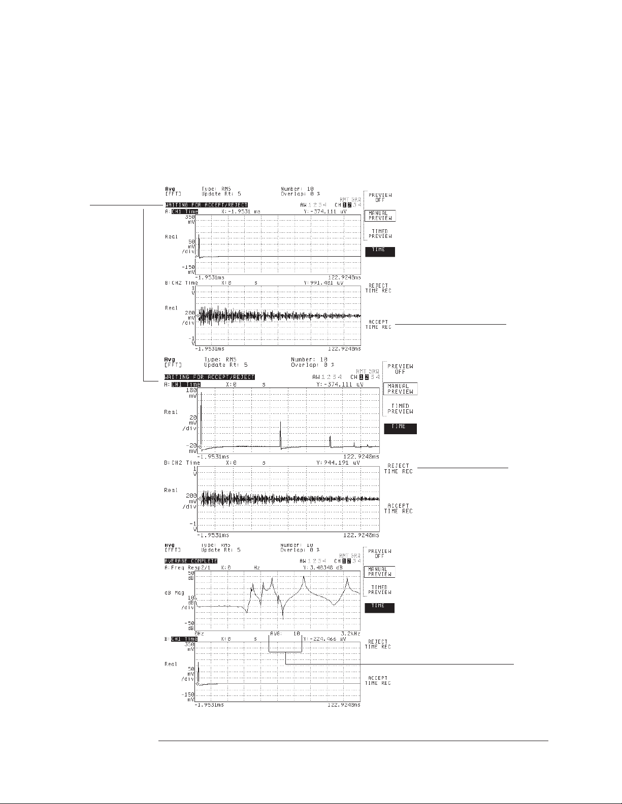
Analyzer is waiting for a response.

Agilent 35670A

Measuring Structures Operator's Guide

If your hammer taps consistently result in overloads, increase the input ranges in step 3 until overloads no longer occur. Specifying a trigger delay in step 4 allows you to see the leading edge of the hammer tap.

When the analyzer receives a trigger, it displays the time record for channel 1 on trace A and the time record for channel 2 on trace B. After you accept the data, the analyzer displays the frequency response on trace A and time channel 1 on trace B.

Press this key to accept the measurement.

2-16

Pressthiskeyto reject the measurement.

Indicates total number of averages.

Page 83

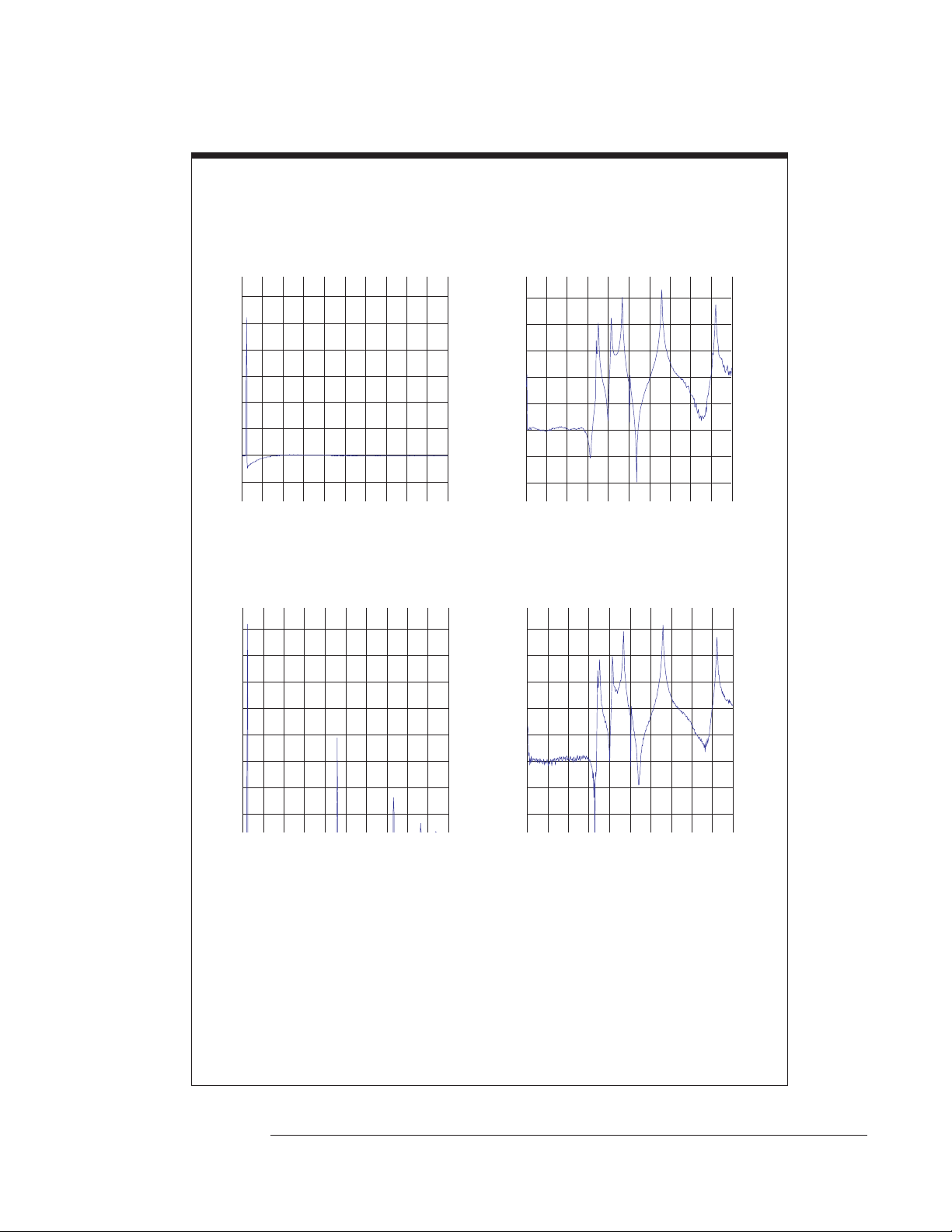
Agilent 35670A Operator's Guide Measuring Structures

When the hammer bounces . . .

Bouncing the hammer during an impact produces a bad measurement. If the measurements are averaged into the modal data during the collection process, the overall modal survey will be in question.

The following traces show the result of a single good hammer tap.

Time domain results of a

good hammer tap

Frequency domain results of a

good hammer tap

The following traces show the result of a multiple impact, such as when the hammer bounces.

Time domain results of a

multiple impact

Frequency domain results of a

multiple impact

The Agilent 35670A’s preview feature allows you to manually or automatically preview the response data from each test before adding it to the average. See online help for more information on manual or timed preview modes.

2-17

Page 84

2-18

Page 85

Measuring Sound

Page 86

Page 87

Measuring Sound

This chapter shows you how to connect and calibrate microphones. It also shows you how to make several typical acoustic measurements. These measurements are made using the analyzer’s octave analysis mode—available only if your analyzer is equipped with Option 1D1.

3-1

Page 88

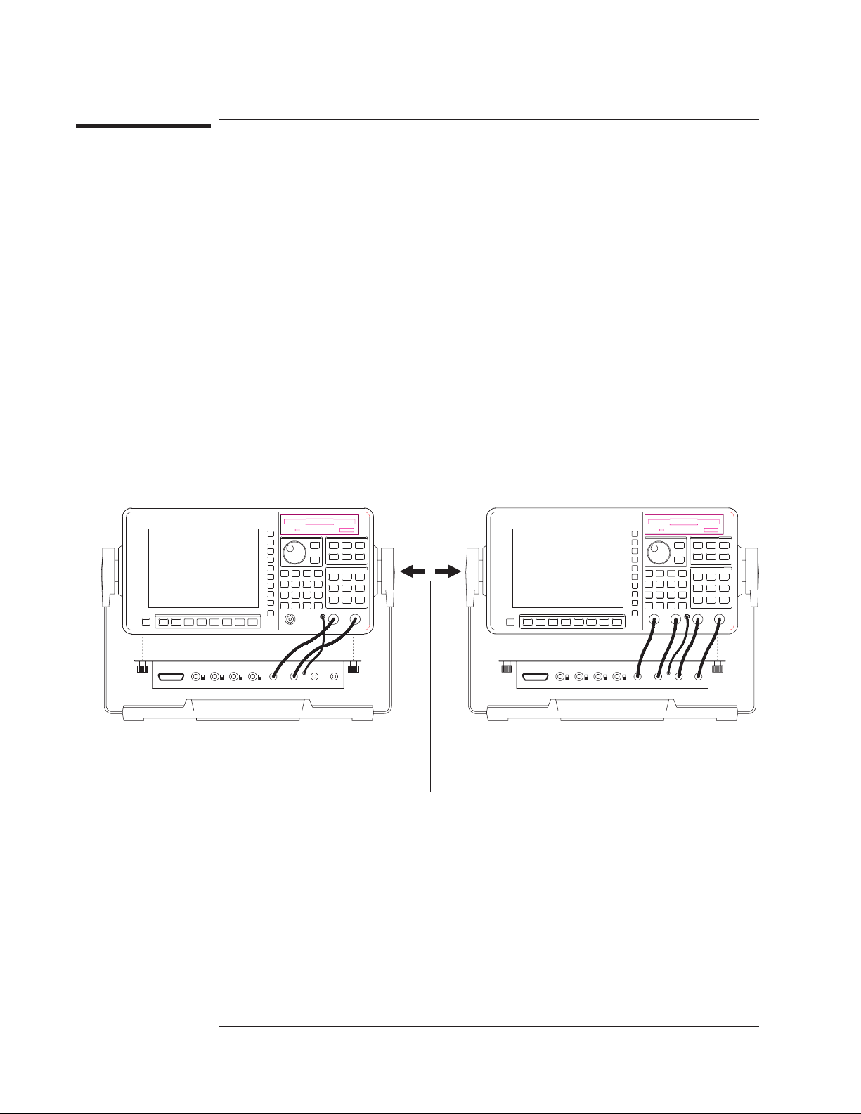
Agilent 35670A

Measuring Sound Operator's Guide

To connect the microphone adapter (Option UK4)

1 Flip the bail handle down to support the front of the analyzer. 2 Insert the threaded ends of the microphone adapter’s two thumbscrews into the holes

on the bottom of the analyzer’s case, then tighten the thumbscrews with your fingers.

3 Attach the microphone adapter’s mic cable to mic connector on the analyzer’s front

panel.

4 Connect the adapter’s BNCs to the corresponding BNCs on the analyzer’s front panel.

The Microphone Adapter and Power Supply (Option UK4) simplifies microphone connections. The mic connector on the analyzer’s front panel provides 8 Vdc to power the adapter. The adapter’s internal power supply uses a step-up converter to provide 28 V and 200 V on the seven-pin input connectors. The 28 V pins power the microphone pre-amplifiers. The 200 V pins polarize the condenser microphone cartridges.

Push in at the pivot points to adjust the bail handle.

Option AY6

3-2

Page 89

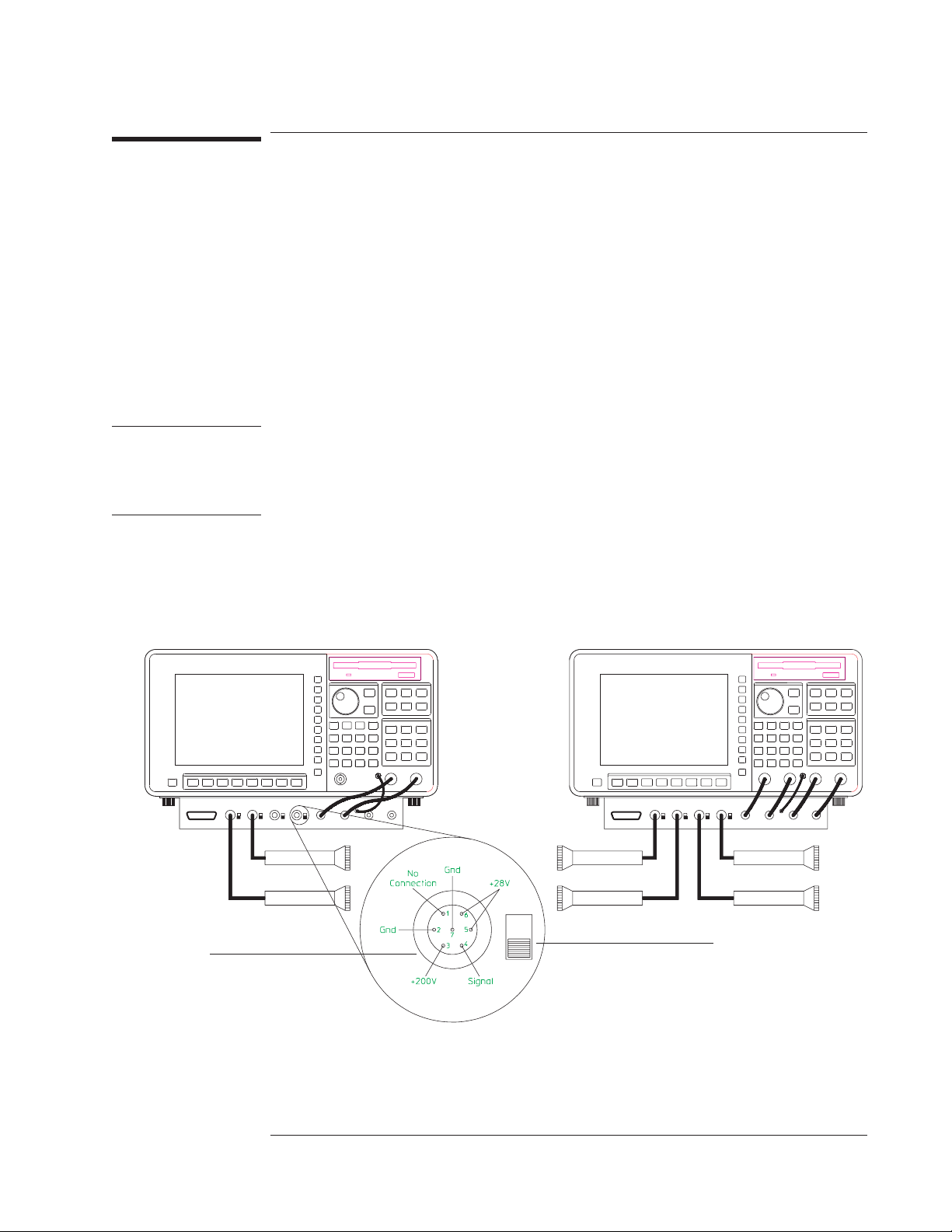
Agilent 35670A Operator's Guide Measuring Sound

To connect microphones

1 Press [

Input

][

ALL CHANNELS][FRONT END CH* SETUP

], then press [

COUPLING AC DC

to highlight AC.

2 If you are using condenser microphones, set the 200 V polarization voltage

switches—located next to the seven-pin input connectors on the microphone power supply—to ON. or If you are using electret (prepolarized condenser) microphones, set the switches to OFF.

3 Attach the microphone output cables to the seven-pin input connectors as shown in the

illustration.

CAUTION Unlike other condenser microphones, electret microphones do not require an external

polarization voltage. To avoid a temporary change in microphone sensitivity (or possible damage), make sure you set the 200 V polarization switch to OFF before attaching an electret microphone to the corresponding seven-pin input connector.

The output signal from a microphone preamplifier usually has a significant dc offset. If the corresponding input channel is dc-coupled, this offset can cause overloads as you increase the channel’s sensitivity. You can prevent dc overloads by selecting ac-coupling.

Option AY6

]

LEMO 18307C connector.

200 V polarization voltage switch.

3-3

Page 90

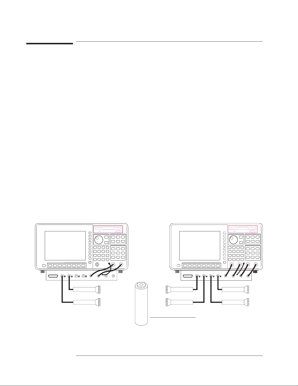
Agilent 35670A

Measuring Sound Operator's Guide

To calibrate a microphone

If you want to accurately measure an acoustic signal, you must enter a calibration factor that tells the analyzer how much voltage is produced at a microphone’s output for a given sound pressure level. In the Agilent 35670A, you enter this factor with the Transducer (Xdcr) Unit softkeys—located under the [

1 Initialize the analyzer.

Press [ Press [ Press [ want activated. Press [ channel whose microphone you will calibrate. Press [

][

Preset Inst Mode

CHANNELS 1 2

Meas Data

PWR SPEC CHANNEL x

DO PRESET

][

OCTAVE ANALYSIS

], then press [

] (or [

CHANNELS 1 2 4

]) to highlight the number of channels you

CHANNEL 1 2

](or[

CHANNEL 1 2 3 4

] to display the microphone output in the active trace.

2 Match the active trace’s display unit to the calibrator’s output unit.

Press [

], then press [

Input

CHANNEL 1 2

whose microphone you will calibrate. Press [

XDCR UNIT CHx SETUP][XDCR UNIT LABEL][Pascal

Press [ Press [ Press [ Press [

], then press [

Rtn

Trace Coord

AMPLITUDE PK PP RMS dB REF SETUP][dBSPL (20 uPa)

XDCR UNIT ON OFF

][

Y UNITS][EU

] to highlight RMS.

] (or [

CHANNEL 1 2 3 4

] to highlight ON.

] hardkey.

Input

]) to highlight the

]) to highlight the channel

3 Connect the microphone adapter and microphone as described in the preceding tasks,

then insert your microphone in the calibrator.

Option AY6

Calibrator.

3-4

Page 91

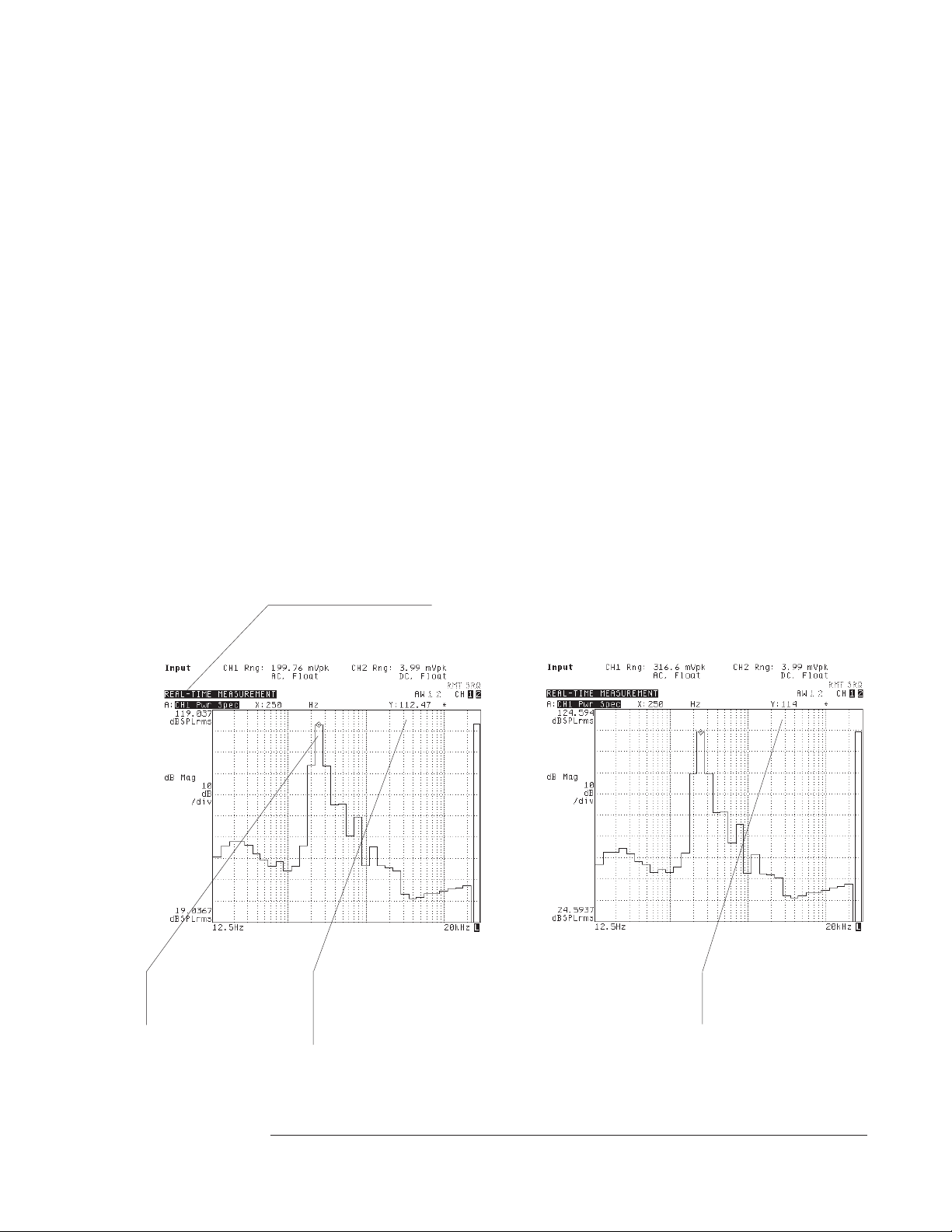
Agilent 35670A Operator's Guide Measuring Sound

4 Specify the measurement and averaging parameters.

Press [ OFF. Press [ greater).

][

Input

Avg

FRONT END CHx SETUP

][

LINEAR][AVERAGE TIME

], then press [

A WT FLTR ON OFF

] to highlight

] <number> [S] (where <number> is 2 or

5 Press [ 6 Turn on the calibrator, then press [

], then press [

Scale

AUTOSCALE ON OFF

Start

] to highlight ON.

7 When the measurement status line says “REAL-TIME MEASUREMENT,” move the

marker to the calibrator’s output frequency and enter calibrator’s output amplitude (in dBSPL).

Press [

Marker

Press [

Input

specified output amplitude (in dBSPL

The analyzer uses the number you enter in [ value for [ accuracy of your microphone measurements. The analyzer automatically stores this value and the [ lost at preset or power-down. However, the values will be used only when [

XDCR UNIT ON OFF

Measurement status line.

][

MARKER TO PEAK

][

XDCR UNIT CHx SETUP][CAL VALUE AT MKR

XDCR SENSITVTY

XDCR UNIT LABEL

)and press [

rms

CAL VALUE AT MKR

]. This new value is the calibration factor that ensures the

] value in nonvolatile memory, so they will not be

] is set to ON.

], then type the calibrator’s

ENTER

] to calculate a new

Marker is placed on calibrator frequency.

Amplitude readout is wrong until you enter the specified calibrator output with [

CAL VALUE AT MKR

Amplitude readout is correct when you complete this task.

3-5

Page 92

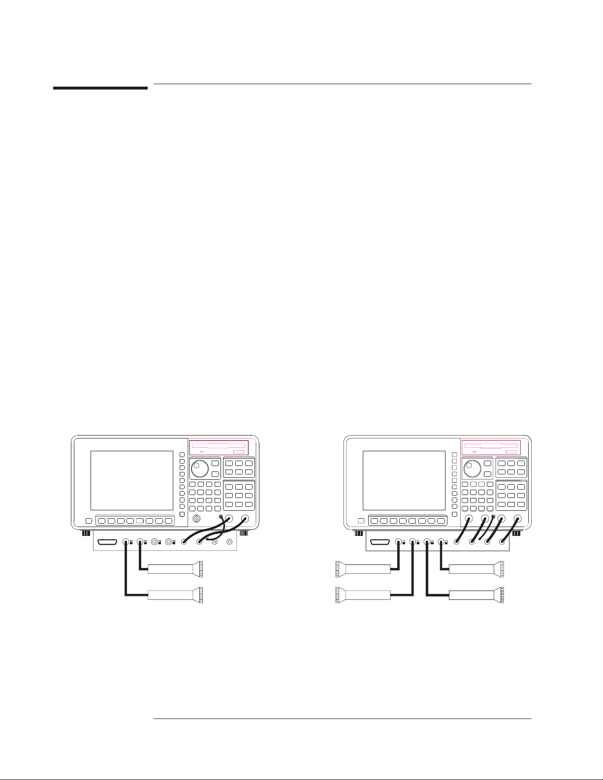
Agilent 35670A

Measuring Sound Operator's Guide

To measure sound pressure level

The Agilent 35670A allows you to measure sound pressure level (SPL) using one of three banks of filters. The filter spacing and bandwidth in these three banks are: one octave (full), one-third octave, and one-twelfth octave. But before you can measure SPL, you must calibrate all the microphones you will use, as shown in the preceding task.

1 Initialize the analyzer.

Complete the preceding task, “To calibrate a microphone.” Press [

Active Trace

you are measuring with two, or [ Press [

Meas Data

microphone’s output to each trace.

2 Set each calibrated microphone in front of an acoustic energy source. 3 Specify the measurement parameters.

Press [ spacing and bandwidth. Press [ range of frequencies you want to measure. Press [ If you want to display A-weighted SPL, press [ [

A WT FLTR ON OFF

], then press [

Freq

START

][

Input

], then press [A] if you are measuring with one microphone, [AB]if

ABCD

][

ALL CHANNELS][PWR SPEC CHANNEL *

1/1 OCTAVE

] <number> <unit>, then press [

ALL CHANNELS][CH* AUTO UP ONLY

] if you are measuring with three or four.

] to assign one

], [

1/3 OCTAVE

], or [

1/12 OCTAVE

] <number> <unit> to select the

STOP

] to select filter

FRONT END CH* SETUP

], then press

] to highlight ON.

Option AY6

3-6

Page 93

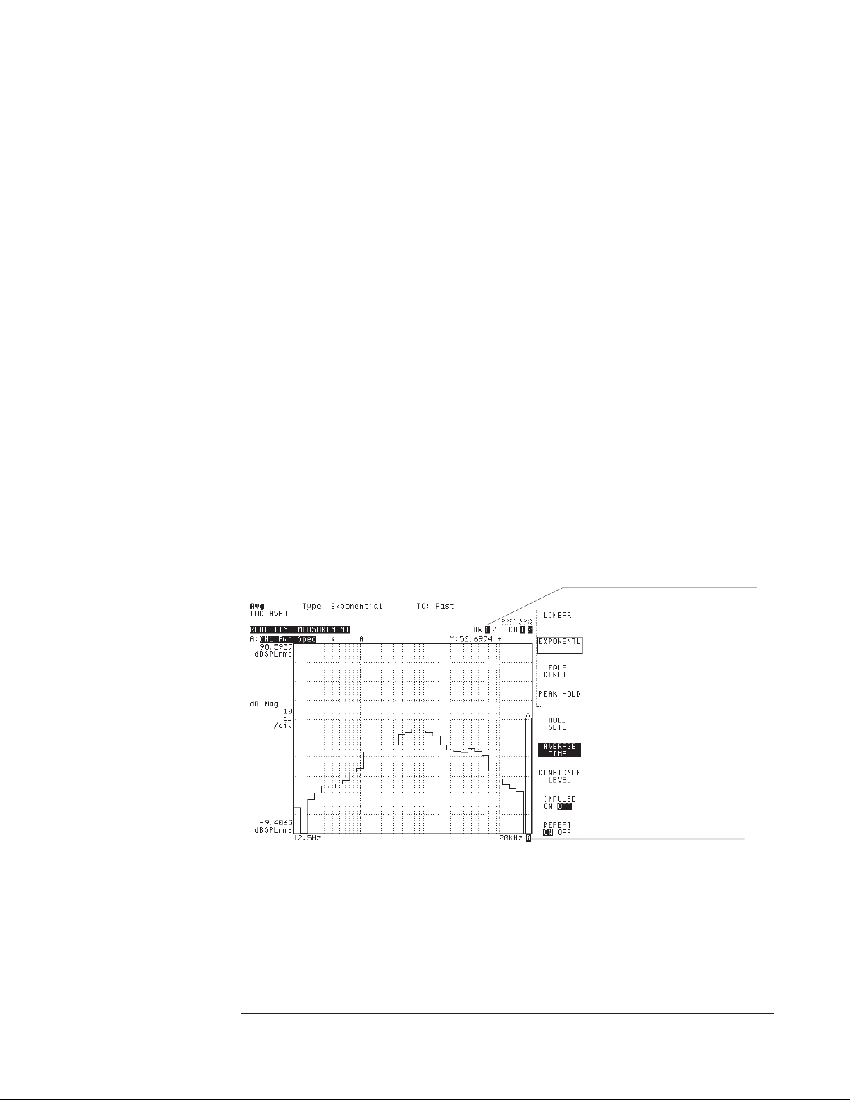
Agilent 35670A Operator's Guide Measuring Sound

4 Specify the averaging parameters.

Press [

If you want to duplicate the LEQfunction of many sound-level meters, press

[

LINEAR

time. If you want to duplicate the “fast” function, press [ [

AVERAGE TIME

If you want to duplicate the “slow” function, press [ [

AVERAGE TIME

Avg

], then press [

] 125 [mS].

]1[S].

AVERAGE TIME

] <number> [

] to specify the integration

ENTER

EXPONENTL

], then press

5 Configure the display.

Press [ highlight ON.

], then press [

Scale

AUTOSCALE ON OFF

] to highlight OFF, and once more to

6 Measure the DUT.

Press [

The analyzer’s A-weight filters conform to ANSI Standard S1.4-1983 and IEC 651-1979, Type 0 Tolerance. An “AW” indicator—located in the upper-right portion of the screen—shows you which channels have their A-weight filters enabled.

Start

You can improve the amplitude accuracy of your measurement by increasing the value of [

AVERAGE TIME

] before you press [

other averaging parameters under the [

]. [

Start

Avg

AVERAGE TIME

] hardkey. See online help for more

] is grouped with several

information on averaging.

Highlighting indicates that channel 1’s A-weight filter is enabled.

Overall band is labeled “A” when A-weight filter is enabled.

3-7

Page 94

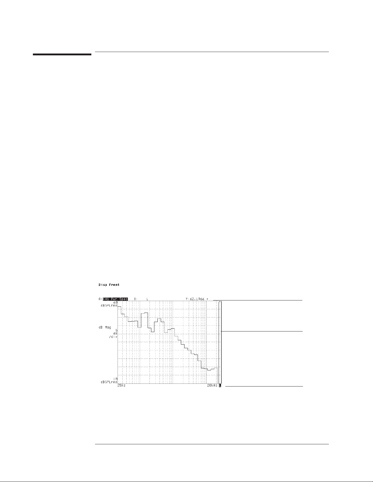
Agilent 35670A

Measuring Sound Operator's Guide

To measure overall sound pressure level

1 Complete the preceding task, “To measure sound pressure level.” 2 If the A-weight filters are on, press [

then press [

3 Press [

AWTFLTRONOFF

Disp Format

][

MORE][OCTAVE BND SETUP

] to highlight OFF.

Input

][

ALL CHANNELS][FRONT END CH* SETUP

], then press [

OVERALL ON OFF

highlight ON.

4 Turn the knob to place the marker on the overall band. 5 Record the marker readout’s Y-axis value.

[

OVERALL ON OFF

displays band-limited overall SPL—the SPL within the current frequency span—if all of the following things are true:

• Linear, exponential, or equal-confidence averaging is selected (under the [

hardkey).

• The impulse detector is turned off (also under the [

• The corresponding channel’s A-weight filter is turned off (under the [

[

FRONT END CHx SETUP

You can also enable a special band that is dedicated to displaying A-weighted, band-limited overall SPL. Just press [ then press [ on either of these two SPL bands.

] enables and disables the analyzer’s overall band. This band

] hardkey).

Avg

]softkey).

][

MORE][OCTAVE BND SETUP

WEIGHTED ON OFF

Disp Format

] to highlight ON. See online help for more information

Input

Avg

]

]to

]

3-8

Marker readout.

Overall band.

“L” indicates band-limited SPL is displayed.

Page 95

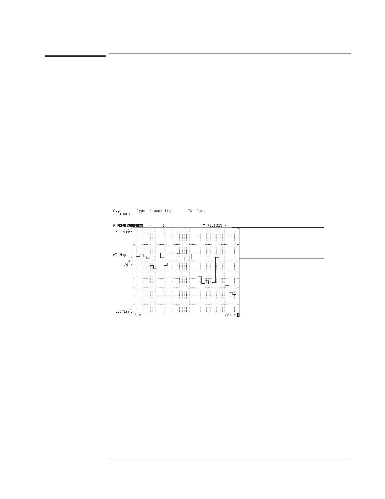
Agilent 35670A Operator's Guide Measuring Sound

To measure overall impulse characteristics

1 Complete the task, “To measure sound pressure level.” 2 Press [ 3 Press [

], then press [

Avg

Disp Format

IMPULSE ON OFF

][

MORE][OCTAVE BND SETUP

] to highlight ON.

], then press [

OVERALL ON OFF

highlight ON.

4 Turn the knob to place the marker on the overall band. 5 Record the marker readout’s Y-axis value.

The overall band displays broadband overall SPL (sound pressure level) with exponential time weighting when the analyzer’s impulse detector is turned on. The displayed value meets the IEC 651 standard for impulse characteristics. Online help for [

IMPULSE ON OFF

] contains a table defining broadband for different analyzer setups.

Marker readout.

Overall band.

]to

“I” indicates broadband impulse characteristics are displayed.

3-9

Page 96

3-10

Page 97

Measuring Spectra and Networks

Page 98

Page 99

Measuring Spectra and Networks

This chapter shows you how to make several typical spectrum and network measurements. Most of the measurements are made using the analyzer’s FFT analysis mode, but one frequency response measurement is made using the swept sine mode—available only if your analyzer is equipped with Option 1D2.

4-1

Page 100

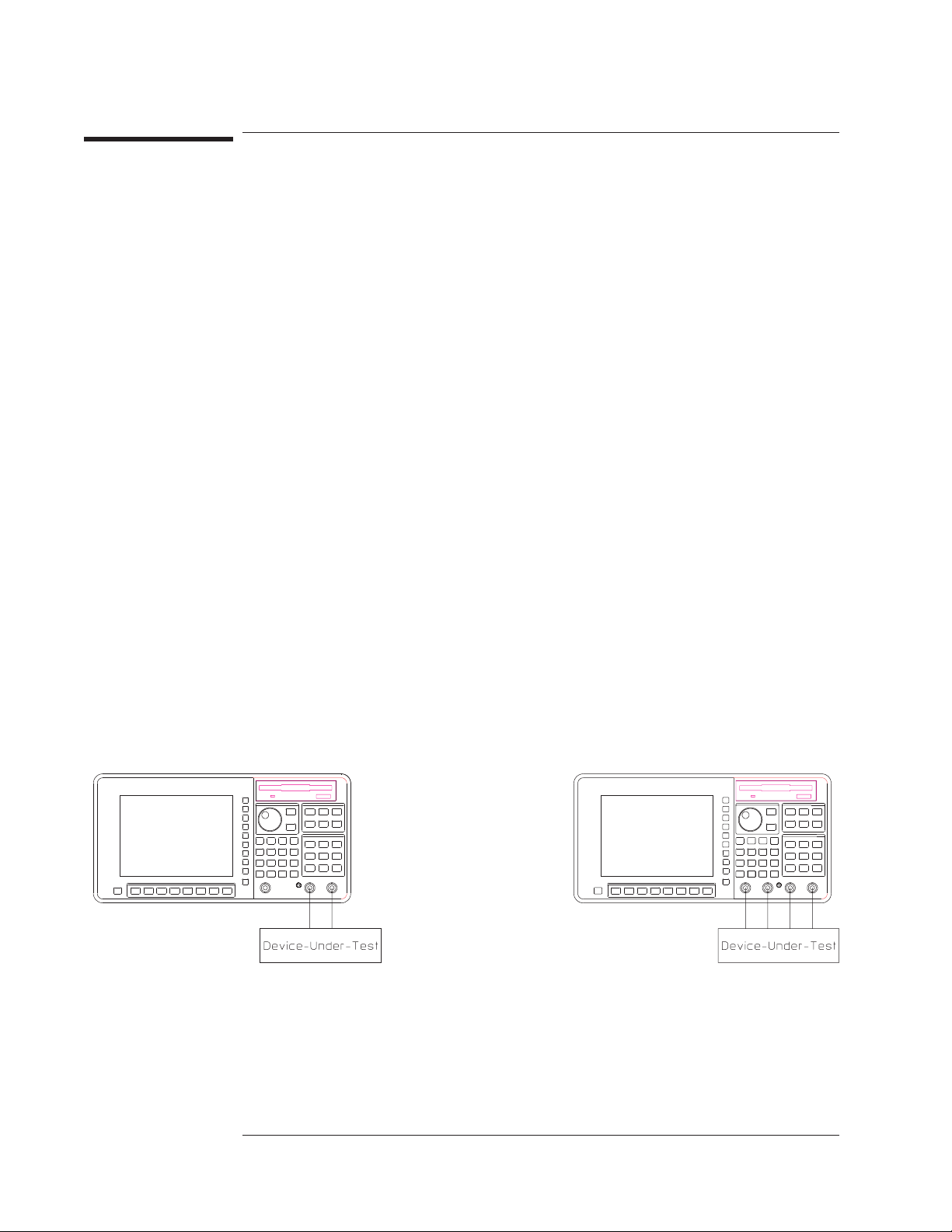
Agilent 35670A

Measuring Spectra and Networks Operator's Guide

To measure a wideband spectrum

You must sometimes survey all frequencies within the analyzer’s measurement range to locate the signal components you want to examine more closely. A two-channel Agilent 35670A, can measure all frequencies between 0 and 102.4 kHz when one channel is active; it can measure between 0 and 51.2 kHz when two channels are active. A four-channel Agilent 35670A can measure all frequencies between 0 and

51.2 kHz when one or two channels are active; it can measure between 0 and 25.6 kHz when four channels are active.

1 Initialize the analyzer.

Press [ Press [ Press [ want activated. Press [ measuringtwo,or[ Press [

2 Connect your test signals to the input connectors (as shown below).

][

Preset Inst Mode

CHANNELS 1 2

Active Trace

Meas Data

DO PRESET

][

FFT ANALYSIS

][

] (or [

CHANNELS 1 2 4

]) to highlight the number of channels you

], then press [A] if you are measuring one signal, [AB] if you are

ABCD

ALL CHANNELS][PWR SPEC CHANNEL *

] if you are measuring three or four.

3 Specify the measurement parameters.

Press [ Press [ If the signals include large dc components, press [ [

FRONT END CH* SETUP

][

Freq Window

FULL SPAN

][

FLAT TOP

], then press [

COUPLING AC DC

][

Input

ALL CHANNELS

] to highlight AC.

]

Option AY6

4-2