Adafruit CircuitPython Libraries and Jupyter Notebook User Manual

CircuitPython Libraries and Jupyter Notebook on any Computer with

MCP2221

Created by Brent Rubell

Last updated on 2021-03-26 10:16:02 AM EDT

2
3

3
3
4

4

4

5
6

6
6
6
8
9
9

10

10

11

11
12

15

15

15

17
17
19

20
20

20

Guide Contents

Guide Contents
Overview

MCP2221
CircuitPython Libraries on your Computer
Jupyter Notebook

Jupyter Notebook is an open-source web application that allows you to create and share documents that contain live code, equations,
visualizations and narrative text.

Parts

Materials
Installing Anaconda

Set up MCP2221
Install Anaconda
Launching Jupyter Notebook
Code Usage
Error: Board not supported None
Error: BLINKA_MCP2221 environment variable set, but no MCP2221 device found

Jupyter Notebook Examples

Compatibility with FT232H

Temperature

Wiring
Code Walkthrough

Accelerometer

Wiring

Code Usage

Increasing the Number of Sensor Readings
Code Walkthrough
About Notebook Performance

Thermal Camera
Wiring

Code Usage

© Adafruit Industries

https://learn.adafruit.com/jupyter-on-any-computer-with-circuitpython-libraries-and-

mcp2221

Page 2 of 23

Overview

This guide will show you how to use Jupyter Notebook with the MCP2221(A) to connect I2C sensors from your desktop PC running Windows, macOS or Linux .
You can use any CircuitPython library for any of our I2C sensors to stream data into your computer's USB port.

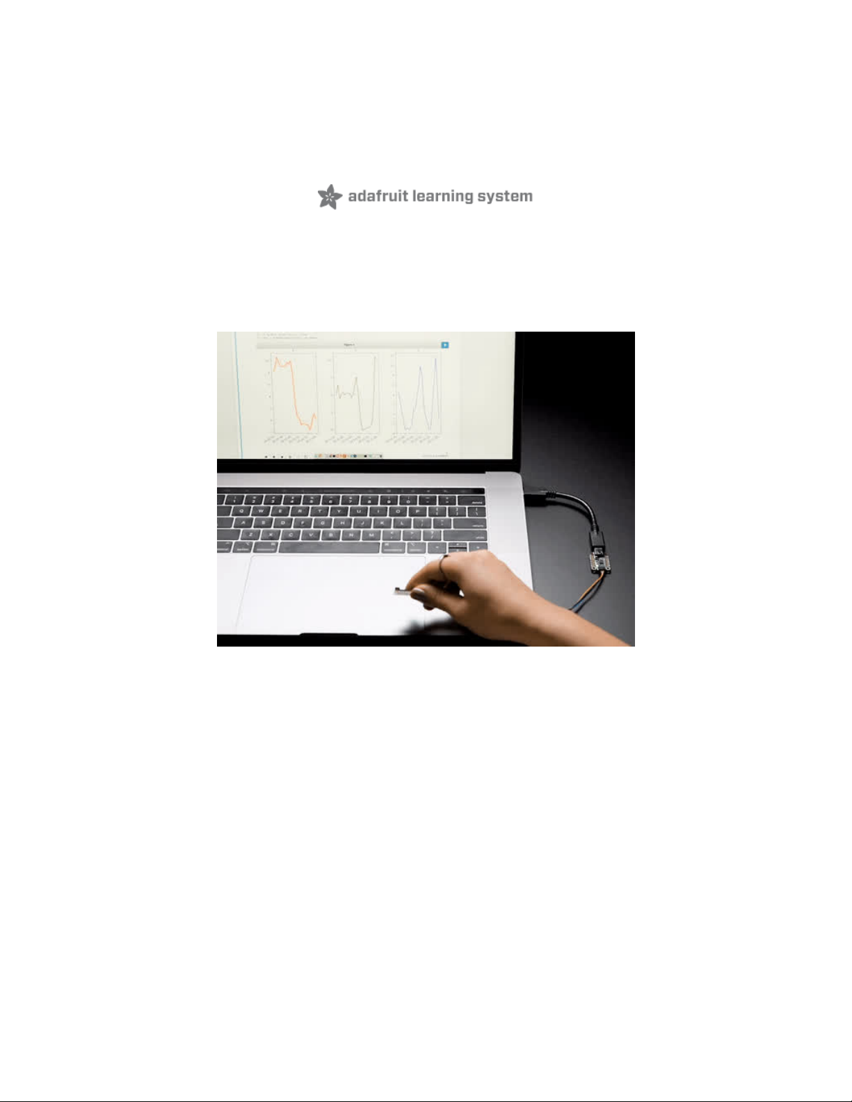
We've written three interactive Jupyter Notebooks for three different types of sensors - a temperature sensor, an accelerometer and a thermal camera. All of these
notebooks have animated graphs so you can see data streaming into your computer in

real-time

.

This guide is also compatible with the Adafruit FT232H breakout (https://adafru.it/xhf) (EXCEPT for the MLX thermal camera example). You'll need to make a
small adjustment to the code. See the Jupyter Notebook Examples page for more information (https://adafru.it/HMf).

MCP2221

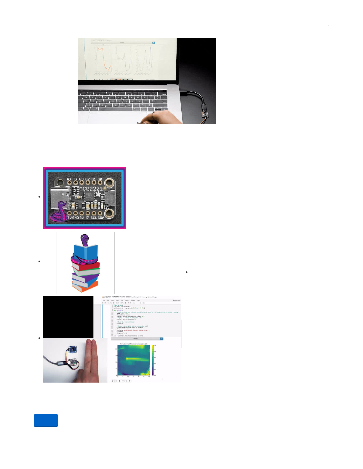
Our MCP2221A breakout board (https://adafru.it/HMA) allows your computer to talk to
sensors or devices that use I2C or analog/digital GPIO.

There's no firmware to deal with, so you don't have to deal with how to "send data to and
from an Arduino which is then sent to and from" an electronic sensor or display or part.

This board is plug & play compatible with with all of our Stemma QT/Qwiic connector

sensors with no soldering required (https://adafru.it/HMB).

CircuitPython Libraries on your Computer

In this guide we will not be using the actual CircuitPython firmware. But we will be installing
and using CircuitPython Libraries on your Computer. This allows us to interface with a
growing collection of 200+ libraries and drivers.

For more information about how this works, check out the CircuitPython Libraries on
MCP2221 Guide here... (https://adafru.it/HMC)

Jupyter Notebook

Jupyter Notebook is an open-source web application that
allows you to create and share documents that contain live
code, equations, visualizations and narrative text.

You'll use Jupyter to create interactive notebooks containing live code which interfaces with
your MCP2221 and sensors.

Parts

Your browser does not support the video tag.
Adafruit MCP2221A Breakout - General Purpose USB to GPIO ADC I2C

Wouldn't it be cool to drive a tiny OLED display, read a
Out of Stock

Out of

Stock

© Adafruit Industries

https://learn.adafruit.com/jupyter-on-any-computer-with-circuitpython-libraries-and-

mcp2221

Page 3 of 23

Adafruit PCT2075 Temperature Sensor - STEMMA QT / Qwiic

The Adafruit PCT2075 Temperature Sensor is a 'code compatible' drop-in replacement for a very...
$4.95
In Stock

Your browser does not support the video tag.
Adafruit LSM6DSOX 6 DoF Accelerometer and Gyroscope

Behold, the ST LSM6DSOX: The latest in a long line of quality Accelerometer+Gyroscope 6-DOF IMUs from ST.This IMU sensor has 6 degrees of freedom - 3
degrees each of linear...
$11.95
In Stock

Your browser does not support the video tag.
Adafruit MLX90640 24x32 IR Thermal Camera Breakout

You can now add affordable heat-vision to your project and with an Adafruit MLX90640 Thermal Camera Breakout. This sensor contains a 24x32 array of IR
thermal sensors. When connected...
Out of Stock

Materials

The MCP2221A has a USB-C connector, make sure you pick up the correct cable or adapter for your computer.

1 x USB C to USB C Cable, 1 meter
USB C to USB C Cable - USB 3.1 Gen 4 with E-Mark - 1 meter long

1 x Micro B USB to USB C Adapter
Micro B USB to USB C Adapter

The sensors we selected for this guide can be used with a STEMMA QT cable so you can plug-and-play with the MCP2221's STEMMA QT port.

1 x STEMMA QT Cable, 50mm
STEMMA QT / Qwiic JST SH 4-Pin Cable - 50mm Long

1 x STEMMA QT Cable, 100mm
STEMMA QT / Qwiic JST SH 4-pin Cable - 100mm Long

1 x STEMMA QT Cable, 200mm
STEMMA QT / Qwiic JST SH 4-Pin Cable - 200mm Long

1 x STEMMA QT to Male Headers Cable, 150mm
STEMMA QT / Qwiic JST SH 4-pin to Premium Male Headers Cable - 150mm Long

Add to Cart

Add to Cart

Out of

Stock

Add to Cart

Add to Cart

Add to Cart

Add to Cart

Add to Cart

Out of

Stock

© Adafruit Industries

https://learn.adafruit.com/jupyter-on-any-computer-with-circuitpython-libraries-and-

mcp2221

Page 4 of 23

Installing Anaconda

Set up MCP2221

This guide assumes you've set up your computer to interface with the MCP2221. If you have not yet set up the MCP2221 for your computer, click the link below
and come back to this page once you have everything set up.

MCP2221 Setup Page (https://adafru.it/HMD)

Install Anaconda

If you're new to all this, the Jupyter Project recommends installing Anaconda (https://adafru.it/HME). This package installs the latest stable version of Python,
Jupyter Notebook, and other commonly used packages for scientific computing and data science.

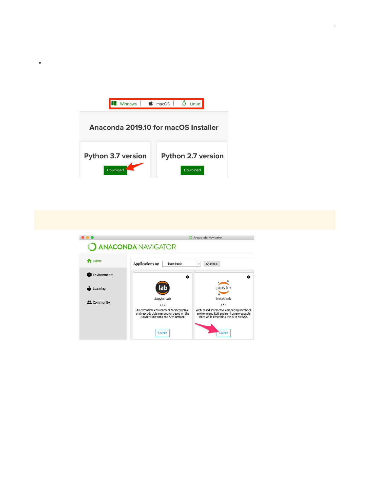
Navigate to the Anaconda downloads page (https://adafru.it/FrB), select your operating system , and download the installer including Python 3.7+.

Install the version of Anaconda you downloaded by following the executable's instructions.

Launching Jupyter Notebook

Once Anaconda is installed, open the Anaconda Navigator Application.

Under Jupyter Notebook, click Launch

 We are using Jupyter Notebook for this guide. At the time of writing, Jupyter Lab has problems with displaying Matplotlib's interactive elements and real-time
data animations and is not recommended for this guide.

Jupyter Notebook should open in a new web browser at the URL http://localhost:8888/notebooks (). To ensure you set up the MCP2221 correctly, we created a
Jupyter Notebook.

Download all the notebooks required for this project by clicking

Download: Project ZIP

on the upper left hand side of the embedded preview below.

Once downloaded, unzip the file and keep it somewhere safe like on your desktop.

© Adafruit Industries

https://learn.adafruit.com/jupyter-on-any-computer-with-circuitpython-libraries-and-

mcp2221

Page 5 of 23

{
"cells": [
{
"cell_type": "code",
"execution_count": null,
"metadata": {},
"outputs": [],
"source": [
"# Python Software Package I nstallation\n",
"import sys\n",
"!{sys.executable} -m pip in stall adafruit-blinka adafruit-ci rcuitpython-msa301 hidapi"
]
},
{
"cell_type": "code",
"execution_count": null,
"metadata": {},
"outputs": [],
"source": [
"# Set an Environment Variab le so Adafruit Blinka knows we're using the MCP2221\n",
"import os\n",
"os.environ[\"BLINKA_MCP2221 \"] = \"1\""
]
},
{
"cell_type": "code",
"execution_count": null,
"metadata": {},
"outputs": [],
"source": [
"# Attempt to import a Circu itPython Module\n",
"import board"
]
}
],
"metadata": {
"kernelspec": {
"display_name": "Python 3",
"language": "python",
"name": "python3"
},
"language_info": {
"codemirror_mode": {
"name": "ipython",
"version": 3
},
"file_extension": ".py",
"mimetype": "text/x-python",
"name": "python",
"nbconvert_exporter": "python ",
"pygments_lexer": "ipython3",
"version": "3.7.4"
}
},
"nbformat": 4,
"nbformat_minor": 2
}

© Adafruit Industries

https://learn.adafruit.com/jupyter-on-any-computer-with-circuitpython-libraries-and-

mcp2221

Page 6 of 23

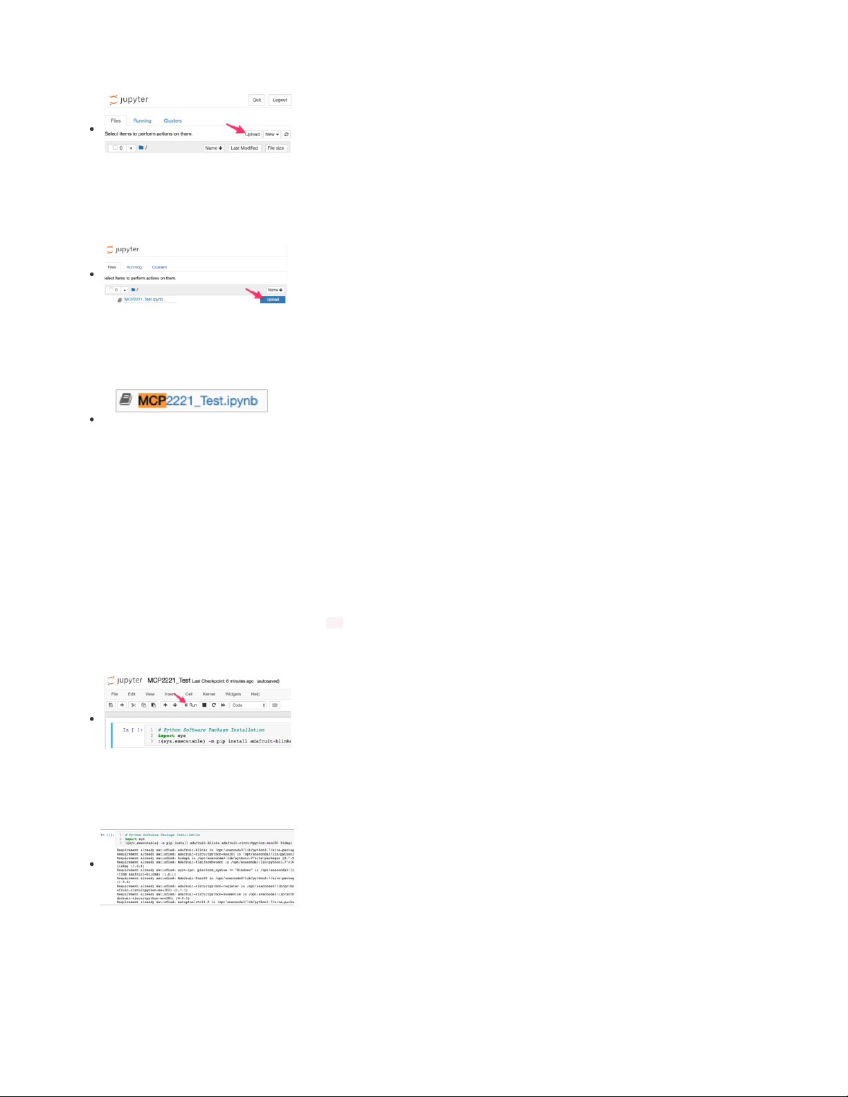
From Jupyter, click the Upload button.

From your file browser, navigate to and select the MCP2221_Test.ipynb file.

The Jupyter notebook should appear in the file browser. Click upload.

Once the Jupyter Notebook has been successfully uploaded, it will show up in the file browser. Click MCP2221_Test.ipynb to
launch the notebook.

Code Usage

Jupyter Notebooks are split into cells. Cells may contain code, images, equations or text. This example notebook only contains code cells.

The first code cell contains two lines. The first imports the sys module which imports functions that interact with the Python interpreter. The second line installs all
the dependencies we need to use this notebook with the MCP2221, including adafruit-blinka and hardware support packages.

To execute this cell, click the first "cell" containing code. Click the run button to execute the code within the cell.

You should observe the output from the Python interpreter print out underneath the cell. Once complete, the cell should
display a

[1]

next to it, indicating the interpreter has completed executing the cell.

© Adafruit Industries

https://learn.adafruit.com/jupyter-on-any-computer-with-circuitpython-libraries-and-

mcp2221

Page 7 of 23

The next cell will set an Environment Variable ( BLINKA_MCP2221 ) so Adafruit Blinka knows we're using the MCP2221
board. Click the cell to highlight it, then click the run button or press ctrl/cmd+enter to execute the code within the cell.

You should get no errors at all, in which case you can continue onto the examples!

Error: Board not supported None

If you get NotImplementedError: Board not supported None ,

That could mean you did not set the MCP2221 environmental variable or you don't have the latest Python libraries installed or the MCP2221 is not plugged in to
USB.

Error: BLINKA_MCP2221 environment variable set, but no MCP2221 device found

If you get this error, check your USB cable - it could be that you have a charge-only not charge+sync cable. Your board may also be unplugged from USB.

© Adafruit Industries

https://learn.adafruit.com/jupyter-on-any-computer-with-circuitpython-libraries-and-

mcp2221

Page 8 of 23

Jupyter Notebook Examples

Now that you have Jupyter installed and Blinka set up on your computer, let's play around!

The following pages contain code examples as downloadable Jupyter notebooks. The examples use some popular sensors we have and should serve as a jumping
off point for your experimentation.

If you're looking for

more sensors

- check out our growing range of plug-and-play STEMMA sensors here (https://adafru.it/HMF). Most of these have CircuitPython

libraries available and are compatible with this guide.

 Make sure you've set the BLINKA_MCP2221 environment variable at the top of your Jupyter Notebooks!

Compatibility with FT232H

The notebooks in this guide are also compatible with the Adafruit FT232H breakout (https://adafru.it/xhf) and CircuitPython Libraries.

If you're using a FT232H breakout, make sure you change the BLINKA_MCP2221 environment variable to BLINKA_FT232H.

Read the learning system guide here to get set up with the FT232H and CircuitPython Libraries... (https://adafru.it/FWD)

© Adafruit Industries

https://learn.adafruit.com/jupyter-on-any-computer-with-circuitpython-libraries-and-

mcp2221

Page 9 of 23

Temperature

This example is a Jupyter notebook which graphs the current temperature using a PCT2075 (https://adafru.it/HDi) temperature sensor. The graph is updated in
real-time with temperature values and we've added horizontal lines across the X-axis to show temperature maximum and minimum thresholds.

While this notebook is designed for the PCT2075 sensor, you can easily implement one of the many temperature sensors available on the Adafruit website. Be
sure to check if it has a CircuitPython library first!

Adafruit PCT2075 Temperature Sensor - STEMMA QT / Qwiic

The Adafruit PCT2075 Temperature Sensor is a 'code compatible' drop-in replacement for a very...
$4.95
In Stock

STEMMA QT / Qwiic JST SH 4-pin Cable - 100mm Long

This 4-wire cable is a little over 100mm / 4" long and fitted with JST-SH female 4-pin connectors on both ends. Compared with the chunkier JST-PH these are 1mm
pitch instead of...
$0.95
In Stock

Wiring

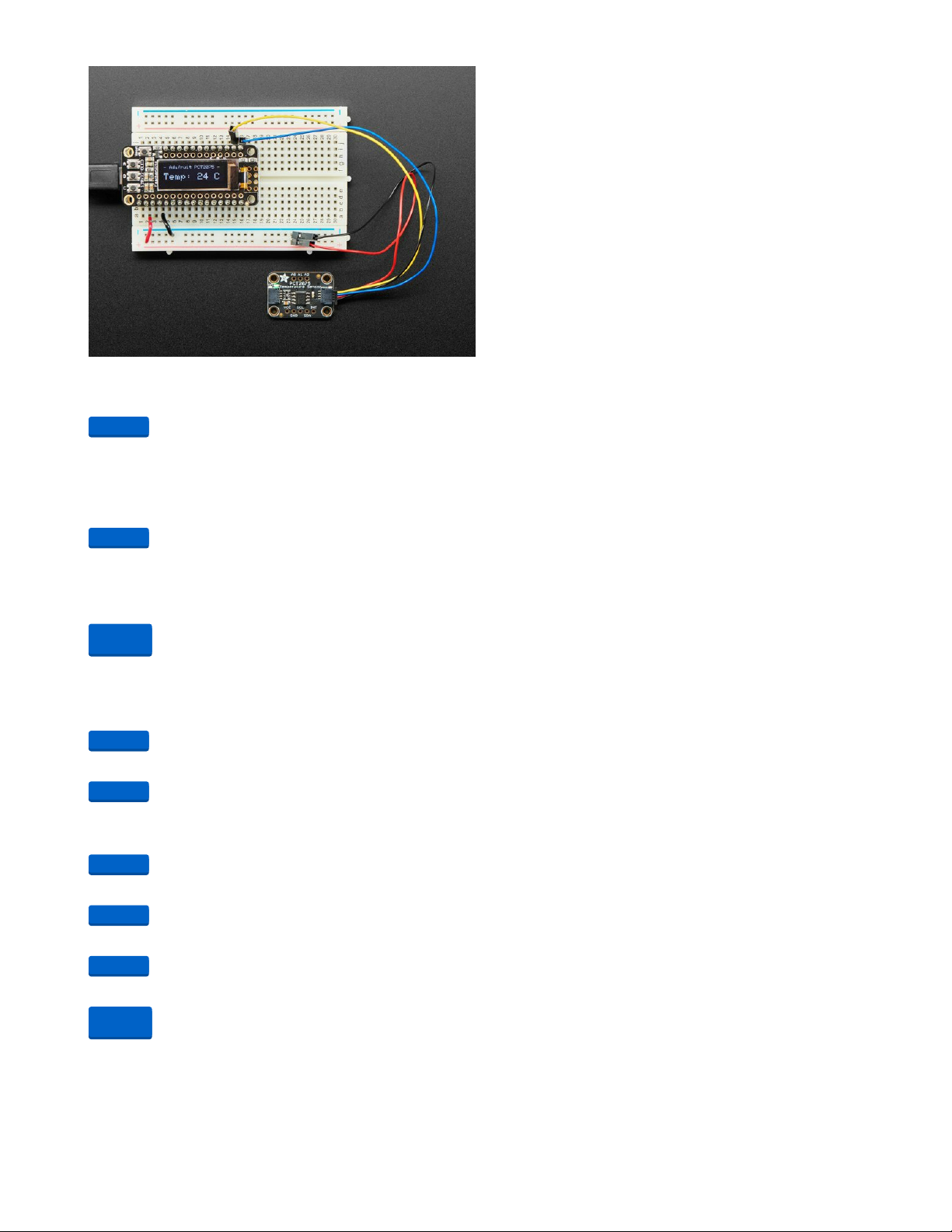
We'll be using the PCT2075 (https://adafru.it/HDi) sensor to precisely measure temperature. The MCP2221 and PCT2075 both have STEMMA QT connectors, so
you can either wire it up on a breadboard or use a STEMMA QT cable.

 Try to avoid hot plugging I2C sensors. The MCP2221 doesn't seem to like that. Remove USB power first.

Add to Cart

Add to Cart

© Adafruit Industries

https://learn.adafruit.com/jupyter-on-any-computer-with-circuitpython-libraries-and-

mcp2221

Page 10 of 23

Make the following connections between the MCP2221 and the
PCT2075:

Board 3V to sensor VCC (red wire )
Board GND to sensor GND (black wire)
Board SCL to sensor SCL (blue wire)
Board SDA to sensor SDA (yellow wire)

Then, download the example notebook:

https://adafru.it/RnD

In the Jupyter file browser, click Upload. From the file browser, select the

PCT2075.ipynb example.

Click the Run button to execute the first cell. This cell will install the adafruit-circuitpython-pct2075 library required for this

example and set an environment variable so Blinka knows we're using the MCP2221

The next cell imports CircuitPython modules (such as board and busio ) and initializes the I2C connection with the sensor. To verify that your board is properly
initialized, it will also print a temperature reading from the PCT2075.

Click the cell containing the code to graph the temperature sensor. The graph should update every 5 seconds with a new reading.

Code Walkthrough

Let's walk through this notebook, cell-by-cell, to understand how this code works.

First, we import all the required libraries for the notebook. We'll be using matplotlib to plot the temperature data from our sensor. We'll also invoke the special

%matplotlib notebook magic to tell matplotlib we're using a Jupyter notebook.

%matplotlib notebook
from datetime import datetime
import matplotlib.pyplot as plt
from collections import deque
from matplotlib.animation import FuncAnimation

Next we declare some constants like HISTORY_SIZE (how many sensor samples we're displaying on the graph), and INTERVAL (the graph's update interval, in

https://adafru.it/RnD

© Adafruit Industries

https://learn.adafruit.com/jupyter-on-any-computer-with-circuitpython-libraries-and-

mcp2221

Page 11 of 23

seconds). We'll also declare MAX_TEMP and MIN_TEMP which are used to generate horizontal lines across the x-axis for displaying the maximum and minimum
temperature values.

# How many sensor samples we wan t to store
HISTORY_SIZE = 100

# Graph update interval (in seco nds)
INTERVAL = 5

# Maximum Temperature (in degree s C)
MAX_TEMP = 30

# Minimum Temperature (in degree s C)
MIN_TEMP = 10

Our code plots and displays 100 sensor readings at a time. We store these readings in a list-like object called a deque container datatype (https://adafru.it/HNa). If
you've never seen this datatype before, don't worry - it's very similar to a list object except it's "optimized for fast fixed-length operations" and support a maxlen
argument which sets the maximum possible size of a deque. When the deque grows beyond its maxlen size, it pops objects off of its opposite end (like a FIFO
stack).

We use one deque to store sensor readings ( temp_data ) and another deque to store time-stamps ( x_time )

# Global x-axis array
x_time = deque(maxlen=HISTORY_SI ZE)

# Temperature data
temp_data = deque(maxlen=HISTORY _SIZE)

Next up, let's make a new plot and give it a title.

# Create new plot
fig, ax = plt.subplots()

# Global title
fig.suptitle("PCT2075 Temperatur e", fontsize=14)

In the animate method, we'll poll the temperature sensor and store it in the temp_data deque. Using the CPython datetime module, the code takes the current time
and formats it using strftime for display on the x-axis as ticks.

# Read the temperature sensor an d add the value to the temp_data array
temp_data.append(pct.temperature )

# Grab the datetime, auto-range based on length of accel_x array
x_time.append(datetime.now().str ftime('%M:%S'))

The next chunk of code clears the axis, constrains the y-axis to display a maximum value of 50 degrees celsius and 0 degrees celsius. It also adds a descriptive
label to the Y-Axis.

# Clear axis prior to plotting
ax.cla()

# Constrain the Y-axis
plt.ylim(top=50,bottom=0)

# Y-Axis label
plt.ylabel('Temperature\n(c)')

We'll use the autofmt_date method to rotate and align the x-axis tick labels. Then, let's add a grid so we can see our data better.

fig.autofmt_xdate()
ax.grid(True, linestyle=':', lin ewidth=0.5)

Next up, plot the temperature graph and two dotted horizontal lines across the x-axis to represent maximum and minimum temperature values.

# Add a horizontal minimum line across the X-axis
plt.axhline(y=MAX_TEMP, color='r ', linestyle=':', label='Max. Tem perature')

# Add a horizontal maximum line across the X-axis
plt.axhline(y=MIN_TEMP, color='b ', linestyle=':', label='Min. Tem perature')

Let's add a legend to the graph. This will make it easy to discern which line is which if we look back at it later, or if the notebook is shared with a colleague or
friend.

Matplotlib's ax.legend() method automatically creates a legend for your graph, provided each plot has a label attached to it.

# Add a legend to the graph
ax.legend()

We'll pause the plot's output for INTERVAL seconds

# Pause the plot for INTERVAL se conds
plt.pause(INTERVAL)

Finally, this method "makes an animation by repeatedly calling a function", animate . We provide it the fig we generated earlier and the function we'd like to

© Adafruit Industries

https://learn.adafruit.com/jupyter-on-any-computer-with-circuitpython-libraries-and-

mcp2221

Page 12 of 23

animate.

ani = animation.FuncAnimation(fi g, animate)

© Adafruit Industries

https://learn.adafruit.com/jupyter-on-any-computer-with-circuitpython-libraries-and-

mcp2221

Page 13 of 23

Accelerometer

Wiring

We'll be using the LSM6DSOX sensor to precisely measure acceleration data (https://adafru.it/HNb). The MCP2221 and LSM6DSOX both have STEMMA QT
connectors, so you can either wire it up on a breadboard or use a STEMMA QT cable.

 Try to avoid hot plugging I2C sensors. The MCP2221 doesn't seem to like that. Remove USB power first.

Your browser does not support the video tag.
Adafruit LSM6DSOX 6 DoF Accelerometer and Gyroscope

Behold, the ST LSM6DSOX: The latest in a long line of quality Accelerometer+Gyroscope 6-DOF IMUs from ST.This IMU sensor has 6 degrees of freedom - 3
degrees each of linear...
$11.95
In Stock

STEMMA QT / Qwiic JST SH 4-pin Cable - 100mm Long

This 4-wire cable is a little over 100mm / 4" long and fitted with JST-SH female 4-pin connectors on both ends. Compared with the chunkier JST-PH these are 1mm
pitch instead of...
$0.95
In Stock

Make the following connections between the MCP2221 and the
LSM6DSOX:

Board 3V to sensor VIN (red wire)
Board GND to sensor GND (black wire)
Board SCL to sensor SCL (yellow wire)
Board SDA to sensor SDA (blue wire)

Then, download the example notebook:

https://adafru.it/RnE

Code Usage

In the Jupyter file browser, click Upload. From the file browser, select the

LSM6DSOX_Accel.ipynb example.

Add to Cart

Add to Cart

https://adafru.it/RnE

© Adafruit Industries

https://learn.adafruit.com/jupyter-on-any-computer-with-circuitpython-libraries-and-

mcp2221

Page 14 of 23

Click the Run
button to

execute the
first cell. This
cell installs the
required
libraries for
using this
notebook.

This cell installs
the adafruit-

circuitpython­lsm6dsox library

for interfacing
with the
LSM303 sensor
.

This cell also
installs a
Jupyter
Extension,

ipympl . This

extension
makes it
possible for us
to create
interactive
Matplotlib
graphs from
within a
Jupyter
notebook.

The next cell sets an environment variable so Blinka knows we're using the MCP2221.

Then, it imports CircuitPython libraries and initializes the I2C connection with the sensor.

The next cell imports CircuitPython modules (such as board and busio ) and initializes the i2c connection with the sensor. To verify that your board is properly
initialized, it should also values form the LSM6DSOX's acceleration sensor.

The next cell sets an environment variable so Blinka knows we're using the MCP2221.

Then, it imports CircuitPython modules (such as board and busio ) and initializes the i2c connection with the sensor. To verify
that your board is properly initialized, it should also print values from the LSM6DSOX acceleration sensor.

If you receive an error with the board module, make sure your MCP2221 is plugged into a usb port on your computer.

The third code cell uses Matplotlib to generate a graph for the LSM6DSOX's acceleration data. We used three side-by-side subplots to visualize the X, Y, and Z
axis.

© Adafruit Industries

https://learn.adafruit.com/jupyter-on-any-computer-with-circuitpython-libraries-and-

mcp2221

Page 15 of 23

Increasing the Number of Sensor Readings

By default, this code cell only displays 20 sensor readings. If you want to display more sensor readings on your graph, simply change the value of the

HISTORY_SIZE variable in the code cell and re-run it.

For more information about how this code cell works, read on!

Code Walkthrough

First, we import all required libraries for this code cell. Most of the libraries come from the Matplotlib library. We use this library to plot the data obtained by our
sensor.

%matplotlib notebook
import matplotlib.pyplot as plt
from matplotlib.animation import FuncAnimation
import datetime
import matplotlib.dates as mdate s
from collections import deque

Our code only plots and displays 20 sensor readings at a time. We store these readings in a list-like object called a deque container

datatype (https://adafru.it/HNa). If you've never seen this datatype before, don't worry - it's very similar to a list object except it's "optimized for fast fixed-length

operations" and support a maxlen argument which sets the maximum possible size of a deque. When the deque grows beyond its maxlen size, it pops objects off
of its opposite end (like a FIFO stack).

We'll be using four deque objects to represent the x-axis, the first graph's y-axis (accelerometer's x-axis data), the second graph's y-axis (accelerometer's y-axis
data), and the third graph's y-axis (accelerometer's y-axis data). These deque objects use HISTORY_SIZE as the deque's maxlen . You may increase the amount of
data to display on the graph by increasing HISTORY_SIZE .

# Deque for X-Axis (time)
x_vals = deque(maxlen=HISTORY_SI ZE)

# Deque for Y-Axis (acceleromete r readings)
accel_x = deque(maxlen=HISTORY_S IZE)
accel_y = deque(maxlen=HISTORY_S IZE)
accel_z = deque(maxlen=HISTORY_S IZE)

Next, we'll create three side-by-side sub-plots and call tight_layout to adjust the subplot parameters to give nicer padding between examples.

For more information about spacing matplotlib subplots, check out this guide... (https://adafru.it/HNc)

# Create 3 side-by-side subplots
fig, (ax1, ax2, ax3) = plt.subpl ots(1,3)

# Automatically adjust subplot p arameters for nicer padding betwe en plots
plt.tight_layout()

Let's now take a look at the animate method. This method polls the LSM303's acceleration values and stores them in a tuple named accel_data . Next, the code
appends the values from the tuple to deque objects, accel_x , accel_y , accel_z .

def animate(i):
# Poll the LSM303AGR
accel_data = accel.accelerat ion
# Add the X/Y/Z values to th e accel arrays
accel_x.append(accel_data[0] )
accel_y.append(accel_data[1] )
accel_z.append(accel_data[2] )

We grab the current time (in seconds using CPython's datetime module) and store it in a deque, x_vals .

# Grab the datetime, auto-range based on length of accel_x array
x_vals = [datetime.datetime.now( ) + datetime.timedelta(seconds=i) for i in range(len(accel_x))]

Now we're up to the fun part of this code walkthrough - displaying the graphs. Since we're "animating" the graph, the axis will need to be cleared and re-drawn
each time the animate method runs. Let's clear the three axis, set up grid titles and enable grid lines.

© Adafruit Industries

https://learn.adafruit.com/jupyter-on-any-computer-with-circuitpython-libraries-and-

mcp2221

Page 16 of 23

# Clear all axis
ax1.cla()
ax2.cla()
ax3.cla()

# Set grid titles
ax1.set_title('X', fontsize=10)
ax2.set_title('Y', fontsize=10)
ax3.set_title('Z', fontsize=10)

# Enable subplot grid lines
ax1.grid(True, linewidth=0.5, li nestyle=':')
ax2.grid(True, linewidth=0.5, li nestyle=':')
ax3.grid(True, linewidth=0.5, li nestyle=':')

Since we are displaying a large amount of data on the x-axis, we'll use Matplotlib's autofmt_xdate()

method (https://adafru.it/HNd) to automatically align and roate the x-axis labels.

The first image on the left shows this code without a call to autofmt_xdate while the second image shows a nicely formatted
graph.

Pretty neat, right

Finally, we'll display the sub-plots on the figure by calling ax.plot and specifying the x-axis and y-axis deques. We'll also specify different colors for each graphs to
help us visually identify the sub-graphs.

# Display the sub-plots
ax1.plot(x_vals, accel_x, color= 'r')
ax2.plot(x_vals, accel_y, color= 'g')
ax3.plot(x_vals, accel_z, color= 'b')

Finally, we'll pause the plot's drawing for INTERVAL seconds.

# Pause the plot for INTERVAL se conds
plt.pause(INTERVAL)

About Notebook Performance

Computers with less available resources will render choppy graphs. For reference, all GIFs in this guide were rendered on a
computer with a 2.6GHz i7 and 32GB of RAM.

We can increase the INTERVAL , keeping in mind two things:

1. USB is limited to one transaction per millisecond

2. We are displaying HISTORY_SIZE samples at a time. You may want to decrease the number of samples displayed on
the graph for better performance.

This method "makes an animation by repeatedly calling a function", animate . We provide it the figure we generated earlier and the function we'd like to animate.

© Adafruit Industries

https://learn.adafruit.com/jupyter-on-any-computer-with-circuitpython-libraries-and-

mcp2221

Page 17 of 23

# Update graph every 125ms
ani = FuncAnimation(fig, animate )

© Adafruit Industries

https://learn.adafruit.com/jupyter-on-any-computer-with-circuitpython-libraries-and-

mcp2221

Page 18 of 23

Thermal Camera
Wiring

We'll be using the MLX90640 IR Thermal Camera Breakout (https://adafru.it/HNe) to display an animated image comprised of thermal data to our notebook.

This breakout contains a 24x32 array of IR thermal sensors. When it's connected to the MCP2221, it returns an array of 768 individual infrared temperature readings
over I2C. We'll read these values, manipulate, and display them in our Jupyter Notebook.

The MCP2221 and MLX90640 (https://adafru.it/HNe) both have STEMMA QT connectors, so you can either wire it up on a breadboard or use a STEMMA QT cable.

Your browser does not support the video tag.
Adafruit MLX90640 24x32 IR Thermal Camera Breakout

You can now add affordable heat-vision to your project and with an Adafruit MLX90640 Thermal Camera Breakout. This sensor contains a 24x32 array of IR
thermal sensors. When connected...
Out of Stock

STEMMA QT / Qwiic JST SH 4-pin Cable - 100mm Long

This 4-wire cable is a little over 100mm / 4" long and fitted with JST-SH female 4-pin connectors on both ends. Compared with the chunkier JST-PH these are 1mm
pitch instead of...
$0.95
In Stock

Then, download the example Jupyter notebook:

https://adafru.it/RnF

Code Usage

In the Jupyter file browser, click Upload. From the file browser, select the MLX90640 Thermal Camera.ipynb

example.

Click the Run button to execute the first cell. This cell first sets an environment

variable so Blinka knows we're using the MCP2221 sensor.

Then, it installs the adafruit-circuitpython-mlx90 640 library for interfacing with the
thermal camera breakout .

Out of

Stock

Add to Cart

https://adafru.it/RnF

© Adafruit Industries

https://learn.adafruit.com/jupyter-on-any-computer-with-circuitpython-libraries-and-

mcp2221

Page 19 of 23

The next code cell imports CircuitPython libraries such as board , busio , and

adafruit_mlx90640 . Then, it initializes an I2C connection with the sensor and

creates a mlx object.

We also set the refresh rate to 1HZ for this notebook.

Before continuing, make sure your code prints the MLX was found on I2C.

If it the MCP2221 was unable to detect the MLX breakout, unplug the sensor and
plug it back in. Then, restart the Jupyter kernel by clicking Kernel->Restart.

Click run on the next cell . This cell reads data from the thermal camera and splits it into a 32x24 array of thermal readings. We're using the numpy

package (https://adafru.it/HNf) so we can do perform fast manipulations to the data within the array.

The next cell plots the data read from the previous cell. Click run to see a heatmap of your data .

This sensor reads the data

twice per frame

, in a checker-board pattern, so it's normal to see a checker-board dither effect when moving the sensor around - the

effect isn't noticable when things move slowly.

The final cell in this notebook produces a live heat-map from your thermal camera. Point the camera towards yourself and click run.

Note: This GIF has been sped up (2x), we suggest moving

very

slowly to avoid a dithering effect.

© Adafruit Industries

https://learn.adafruit.com/jupyter-on-any-computer-with-circuitpython-libraries-and-

mcp2221

Page 20 of 23

© Adafruit Industries

https://learn.adafruit.com/jupyter-on-any-computer-with-circuitpython-libraries-and-

mcp2221

Page 21 of 23

© Adafruit Industries

https://learn.adafruit.com/jupyter-on-any-computer-with-circuitpython-libraries-and-

mcp2221

Page 22 of 23

© Adafruit Industries Last Updated: 2021-03-26 10:16:02 AM EDT Page 23 of 23