Velodyne Acoustics HDL-64E S2, HDL-64E S2.1 User Manual

U S E R ’ S M A N U A L A N D

P R O G R A M M I N G G U I D E

Firmware Version 4 . 07

HDL-64E S2

and S2.1

High Definition LiDAR™ Sensor

Last Six Bytes Examples

iS A F E T Y N O T I C E S

1	I N T R O D U C T I O N
	In The Box
2	P R I N C I P L E S O F O P E R A T I O N
3	I N S T A L L A T I O N O V E R V I E W
3	Front/Back Mounting
4	Side Mounting

5Top Mounting

6Wiring

6U S A G E

6Use the Included Point-cloud Viewer

6Develop Your Own Application-specific Point-cloud Viewer

7 db.xml Calibration Parameters

8 Change Run-Time Parameters

10Control Spin Rate

—Change Spin Rate in Flash Memory

—Change Spin Rate in RAM Only

10Limit Horizontal FOV data Collected

11Define Sensor Memory IP Source and Destination Addresses

11 Upload Calibration Data

11External GPS Time Synchronization

—GPS Receiver Option 1: Velodyne Supplied GPS Receiver

—GPS Receiver Option 2: Customer Supplied GPS Receiver

13Packet Format and Status Byte for GPS Time Stamping

13	Time Stamping Accuracy Rules
13	Laser Firing Sequence and Timing
14	F I R M W A R E U P D A T E
15	A P P E N D I X A : Mechanical Drawings

16A P P E N D I X B : Wiring Diagram

17A P P E N D I X C : Digital Sensor Recorder (DSR)

17	Install
17	Calibrate

17Live Playback

18Record Data

18Playback of Recorded Files

19DSR Key Controls

19DSR Mouse Controls

20A P P E N D I X D : Matlab Sample Code

22Reading Calibration and Sensor Parameter Data

23A P P E N D I X E : Data Packet Format

27

30	A P P E N D I X	F :	Dual Two Point Calibration Methodology
34	A P P E N D I X	G :	Ethernet Transmit Timing Table

36A P P E N D I X H : Laser and Detector Arrangement

37A P P E N D I X I : Angular Resolution

38T R O U B L E S H O O T I N G

38S E R V I C E A N D M A I N T E N A N C E

39S P E C I F I C A T I O N S

caution — safety notice

Caution

To reduce the risk of electric shock and to avoid violating the warranty, do not open sensor body. Refer servicing to qualified service personnel.

The lightning flash with arrowhead symbol is intended to alert the user to the presence of uninsulated “dangerous voltage” within the product’s enclosure that may be of sufficient magnitude to constitute a risk of electric shock to persons.

The exclamation point symbol is intended to alert the user to the presence of important operating and maintenance (servicing) instructions in the literature accompanying the product.

1.Read Instructions — All safety and operating instructions should be read before the product is operated.

2.Retain Instructions — The safety and operating instructions should be retained for future reference.

3.Heed Warnings — All warnings on the product and in the operating instructions should be adhered to.

4.Follow Instructions — All operating and use instructions should be followed.

5.Servicing — The user should not attempt to service the product beyond what is described in the operating instructions. All other servicing should be referred to Velodyne.

1

[ i ]

introduction

HDL-64E S2 and S2.1 User’s Manual

Congratulations on your purchase of a Velodyne HDL-64E S2 or S2.1 High Definition LiDAR Sensor. These sensors represent a breakthrough in sensing technology by providing more information about the surrounding environment than previously possible. The HDL-64E S2 or S2.1 High Definition LiDAR sensors are referred to as the sensor throughout this manual.

This manual and programming guide covers:

•Installation and wiring

•HDL-64-ADAPT (GPS Adaptor Box)

•The data packet format

•The serial interface

•Software updates

•GPS installation notes

•Viewing the data

•Programming information

This manual applies to the two versions of the HDL-64E sensor, the S2 and S2.1, unless otherwise indicated. The table below compares the laser layout, vertical field of view (VFOV) and primary application of the two versions.

HDL-64E Version	Lower Laser Block		Upper Laser Block	Vertical Field of View (VFOV)	Primary Application
S2	32 lasers separated by		32 lasers separated by	+2 to -24.8°	Autonomous navigation
	½° vertical spacing		1/3° vertical spacing
S2.1	32 lasers separated by		32 lasers separated by	31.5°	3D mapping
(dual lower block)	½° vertical spacing		½° vertical spacing

For the latest updates to this manual – check www.velodynelidar.com.

In the Box

Each shipment contains:

•Sensor

•HDL-64-ADAPT (GPS Adaptor Box)

•Wiring harness

•CD with user manual, calibration file (db.xml), timing table calculation file (.xls) and DSR viewer

[ 1 ]

PrinciPLes of oPeration

HDL-64E S2 and S2.1 User’s Manual

The sensor operates, instead of a single laser firing through a rotating mirror, with 64 lasers fixed mounted on upper and lower laser blocks, each housing 32 lasers. Both laser blocks rotate as a single unit. With this design each of the lasers fires tens of thousands of times per second, providing exponentially more data points/second and a more data-intensive point cloud than a rotating mirror design. The sensor delivers a 360° horizontal Field of View (HFOV) and a 26.8° vertical FOV (31.5° VFOV for the S2.1).

Additionally, state-of-the-art digital signal processing and waveform analysis are employed to provide high accuracy, extended distance sensing and intensity data. The sensor is rated to provide usable returns up to 120 meters. The sensor employs a direct drive motor system with no belts or chains in the drive train.

See the specifications at the end of this manual for more information about sensor operating conditions.

Laser

Emitters

(Groups of 16)

Laser

Receivers

(Groups of 32)

Motor

Housing

Figure 1. HDL-64E S2 design overview.

Housing

(Entire unit spins at 5-20 Hz)

[ 2 ]

instaLLation oVerVieW

HDL-64E S2 and S2.1 User’s Manual

The sensor base provides the following mounting options:

•Front/Back mount (Figure 2)

•Side mount (Figure 3)

•Top mount (Figure 4)

The sensor can be mounted at any angle from 0 to 90° with respect to its base. Refer to Appendix A for complete dimensions. For all mounting options, mount the sensor to withstand vibration and shock without risk of detachment. Although helpful for longer life, the unit doesn’t need to be shock proofed as it’s designed to withstand standard automotive G-forces.

The sensor is weatherproofed to withstand wind, rain and other adverse weather conditions. The spinning of the sensor helps it shed excess water from the front window that could hamper performance.

Front/Back Mounting

[152.4mm]

6.00

[203.2mm]

8.00

[21mm]

.83

[25.4mm]

1.00

Two M8-1.25mm x 12mm deep mounting points. (Two per side, for a total of 8.)

Mounting

Base

Figure 2. Front and back HDL mounting illustration.

[ 3 ]

instaLLation oVerVieW

HDL-64E S2 and S2.1 User’s Manual

Side Mounting

Mounting

Base

[152.4mm]

6.00

[203.2mm]

8.00

[21mm] [25.4mm]

.83 1.00

Figure 3. Side HDL mounting illustration.

[ 4 ]

instaLLation oVerVieW

HDL-64E S2 and S2.1 User’s Manual

Top Mounting

[33.8mm]

1.33

[177.8mm]

7.00

[12.7mm]
.50		[12.7mm]
		.50

Figure 4. Top HDL mounting illustration.

Four 0.41” [10.3mm] through holes for top mount option to secure the HDL to the vehicle.

[177.8mm]

7.00

[ 5 ]

instaLLation oVerVieW

HDL-64E S2 and S2.1 User’s Manual

Wiring

The sensor comes with a pre-wired connector, wired with power, DB9 serial and standard RJ45 Ethernet connectors. The connector wires are approximately 10’ [3 meters] in length.

Power. Connect the red and black wires to vehicle power. Be sure red is positive polarity. THE SENSOR IS RATED ONLY FOR 12 - 16 VOLTS. Any voltage applied over 16 volts could damage the sensor. The sensor draws 4-6 AMPS during normal usage.

The sensor doesn’t have a power switch. It spins whenever power is applied.

Lockout Circuit. The sensor has a lockout circuit that prevents its lasers from firing until it achieves approximately 300 RPMs.

Ethernet. This standard Ethernet connector is designed to connect to a standard PC.

The sensor is only compatible with network cards that have either MDI or AUTO MDIX capability.

Serial Interface RS-232 DB9. This standard connector allows for a firmware update to be applied to the sensor. Velodyne may release firmware updates from time to time. It also accepts commands to change the RPM of the unit, control HFOV, change the unit’s IP address, and other functions described later in this manual.

Wiring Diagram. If you need to wire your own connector for your installation, refer to the wiring diagram in Appendix B.

usaGe

The sensor needs no configuration, calibration, or other setup to begin producing usable data. Once the unit is mounted and wired, supplying it power causes it to start scanning and producing data packets.

Use the Included Point-cloud Viewer

The quickest way to view the data collected as an image is to use the included Digital Sensor Recorder (DSR). DSR is Velodyne’s point-cloud processing data viewer software. DSR reads in the packets from the sensor over Ethernet, performs the necessary calculations to determine point locations and then plots the points in 3D on your PC monitor. You can observe both distance and intensity data through DSR. If you have never used the sensor before, this is the recommended starting point. For more on installing and using DSR, see Appendix C.

Develop Your Own Application-specific Point-cloud Viewer

Many users elect to develop their own application-specific point cloud tracking and plotting and/or storage scheme, which requires these fundamental steps:

1.Establish communication with the sensor.

2.Create a calibration table either from the calibration data included in-stream from the sensor or from the included db.xml data file.

3.Parse the packets for rotation, block, distance and intensity data

4.Apply the calibration factors to the data.

5.Plot or store the data as needed.

[ 6 ]

usaGe	HDL-64E S2 and S2.1 User’s Manual

The following provides more detail on each of the above steps.

1. Establish communication with the sensor.

The sensor broadcasts UDP packets. By using a network monitoring tool, such as Wireshark, you can capture and observe the packets as they are generated by the sensor. See Appendix E for the UDP packet format. The default source IP address for the sensor is 192.168.3.043, and the destination IP address is 192.168.3.255. To change these IP addresses, see page 11.

2.Create an internal calibration table either from the calibration data included in-stream from the sensor or from the included db.xml data file.

This table must be built and stored internal to the point-cloud processing software. The easiest and most reliable way to build the calibration table is by reading the calibration data directly from the UDP data packets. A MatLab example of reading and building such a table can be found in Appendix D and on the CD included with the sensor named CALTABLEBUILD.m.

Alternatively, the calibration data can be found in the included db.xml file found on the CD included with the sensor. A description of the calibration data is shown in the following table.

db.xml Calibration Parameters

	Parameter	Unit	Description	Values
	rotCorrection	degree	The rotational correction angle for each laser,	Positive factors rotate to the left.
			as viewed from the back of the unit.	Negative values rotate to
				the right.
	vertCorrection	degree	The vertical correction angle for each laser,	Positive values have the laser
			as viewed from the back of the unit.	pointing up.
				Negative values have the laser
				pointing down.
	distCorrection	cm	Far distance correction of each laser distance	Add directly to the distance value
			due to minor laser parts’ variances.	read in the packet.
	distCorrectionX	cm	Close distance correction in X of each laser due to
			minor laser parts variances interpolated with far
			distance correction then applied to measurement in X.
	distCorrectionY	cm	Close distance correction in Y of each laser due to
			minor laser parts variances interpolated with far
			distance correction then applied to measurement in Y.
	vertOffsetCorrection	cm	The height of each laser as measured from	One fixed value for all upper
			the bottom of the base.	block lasers.
				Another fixed value for all lower
				block lasers.
	horizOffsetCorrection	cm	The horizontal offset of each laser	Fixed positive or negative value
			as viewed from the back of the laser.	for all lasers.
	Maximum Intensity			Value from 0 to 255. Usually 255.
	Minimum Intensity			Value from 0 to 255. Usually 0.
	Focal Distance		Maximum intensity distance.
	Focal Slope		The control intensity amount.

The calibration table, once assembled, contains 64 instances of the calibration values shown in the table above to interpret the packet data to calculate each point’s position in 3D space. Use the first 32 points for the upper block and the second 32 points for the lower block. The rotational info found in the packet header is used to determine the packets position with respect to the 360° horizontal field of view.

[ 7 ]

usaGe	HDL-64E S2 and S2.1 User’s Manual

3.Parse the packets for rotation, block, distance and intensity data. Each sensor’s LIFO data packet has a 1206 byte payload consisting of 12 blocks of 100 byte firing data followed by 6 bytes of calibration and other information pertaining to the sensor.

Each 100 byte record contains a block identifier, then a rotational value followed by 32 3-byte combinations that report on each laser fired for the block. Two bytes report distance to the nearest 0.2 cm, and the remaining byte reports intensity on a scale of 0 -255. 12 100 byte records exist, therefore, 6 records exist for each block in each packet. For more on packet construction, see Appendix E.

4.Apply the calibration factors to the data. Each of the sensor’s lasers is fixed with respect to vertical angle and offset to the rotational index data provided in each packet. For each data point issued by the sensor, rotational and horizontal correction factors must be applied to determine the point’s location in 3D space referred to by the return. Intensity and distance offsets must also be applied. Each sensor comes from Velodyne’s factory calibrated using a dual-point calibration methodology, explained further in Appendix F.

The minimum return distance for the sensor is approximately 3 feet (0.9 meters). Ignore returns closer than this.

A file on the CD called “HDL Source Example” shows the calculations using the above correction factors. This DSR uses this code to determine 3D locations of sensor data points.

5.Plot or store the data as needed. For DSR, the point-cloud data, once determined, is plotted onscreen. The source to do this can be found on the CD and is entitled “HDL Plotting Example.” DSR uses OpenGL to do its plotting.

You may also want to store the data. If so, it may be useful to timestamp the data so it can be referenced and coordinated with other sensor data later. The sensor has the capability to synchronize its data with GPS precision time. For more in this capability, see page 11.

Change Run-Time Parameters

The sensor has several run-time parameters that can be changed using the RS-232 serial port. For all commands, use the following serial parameters:

•Baud 9600

•Parity: None

•Data bits: 8

•Stop bits: 1

All serial commands, except one version of the spin rate command, store data in the sensor’s flash memory. Data stored in flash memory through serial commands is retained during firmware updates or power cycles.

The sensor has no echo back feature, so no serial data is returned from the sensor. Commands can be sent using a terminal program or by using batch files (e.g. .bat). A sample .bat file is shown below.

Sample Batch File (.bat)

MODE COM3: 9600,N,8,1 COPY SERCMD.txt COM3 Pause

Sample SERCMD.txt file

This command sets the spin rate to 300 RPM and stores the new value in the unit’s flash memory.

#HDLRPM0300$

[ 8 ]

usaGe	HDL-64E S2 and S2.1 User’s Manual

Available commands

The following run-time commands are available with the sensor:

Command	Description	Parameters
#HDLRPMnnnn$	Set spin rate from 300 to 1200 RPM	nnnn is an integer between 0300 and 1200
	n flash memory (default is 600 RPM)
#HDLRPNnnnn$	Set spin rate from 300 to 1200 RPM	nnnn is an integer between 0300 and 1200
	in RAM (default is 600 RPM)
#HDLIPAssssssssssssdddddddddddd$	Change source and/or destination	• ssssssssssss is the source 12-digit IP address
	IP address	• dddddddddddd is the destination 12-digit
		IP address
#HDLFOVsssnnn$	Change horizontal Field of View (HFOV)	• sss = starting angle in degrees; sss is an integer
		between 000 and 360
		• nnn = ending angle in degrees; nnn is an
		integer between 000 and 360

You can also upload calibration data from db.xml into flash memory and use GPS time synchronization.

.

[ 9 ]

usaGe	HDL-64E S2 and S2.1 User’s Manual

Control Spin Rate

Change Spin Rate in Flash Memory

The sensor can spin at rates ranging from 300 RPM (5 Hz) to 1200 RPM (20 Hz). The default is 600 RPM (10 Hz). Changing the spin rate does not change the data rate – the unit sends out the same number of packets (at a rate of ~1.3 million data points per second) regardless of its spin rate. The horizontal image resolution increases or decreases depending on rotation speed.

See the Angular Resolution section found in Appendix I for the angular resolution values for various spin rates.

To control the sensor’s spin rate, issue a serial command of the case sensitive format #HDLRPMnnnn$ where nnnn is an integer between 0300 and 1200. The sensor immediately adopts the new spin rate. You don’t need to power cycle the unit, and the new RPM is retained with future power cycles.

Change Spin Rate in RAM Only

If repeated and rapid updates to the RPM are needed, such as for synchronizing multiple sensors controlled by a closed loop application, you can adjust the sensors’ spin rates without storing the new RPM in flash memory (this preserves flash memory over time).

To control the sensor’s spin rate in RAM only, issue a serial command of the case sensitive format #HDLRPNnnnn$ where nnnn is an integer between 0300 and 1200. The sensor immediately adopts the new spin rate. You shouldn’t power cycle the sensor as the new RPM is lost with future power cycles, which returns to the last known RPM.

Limit Horizontal FOV Data Collected

The sensor defaults to a 360° surrounding view of its environment. It may be desirable to reduce this horizontal Field of View (HFOV) and, hence, the data created.

To limit the horizontal FOV, issue a serial command of the case sensitive format #HDLFOVsssnnn$ where:

•sss = starting angle in degrees; sss is an integer between 000 and 360

•nnn = ending angle in degrees; nnn is an integer between 000 and 360

The HDL unit immediately adopts the new HFOV angles without power cycling and will retain the new HFOV settings upon power cycle.

Regardless of the FOV setting, the lasers will always fire at the full 360° HFOV. Limiting the HFOV only limits data transmission to the HFOV of interest.

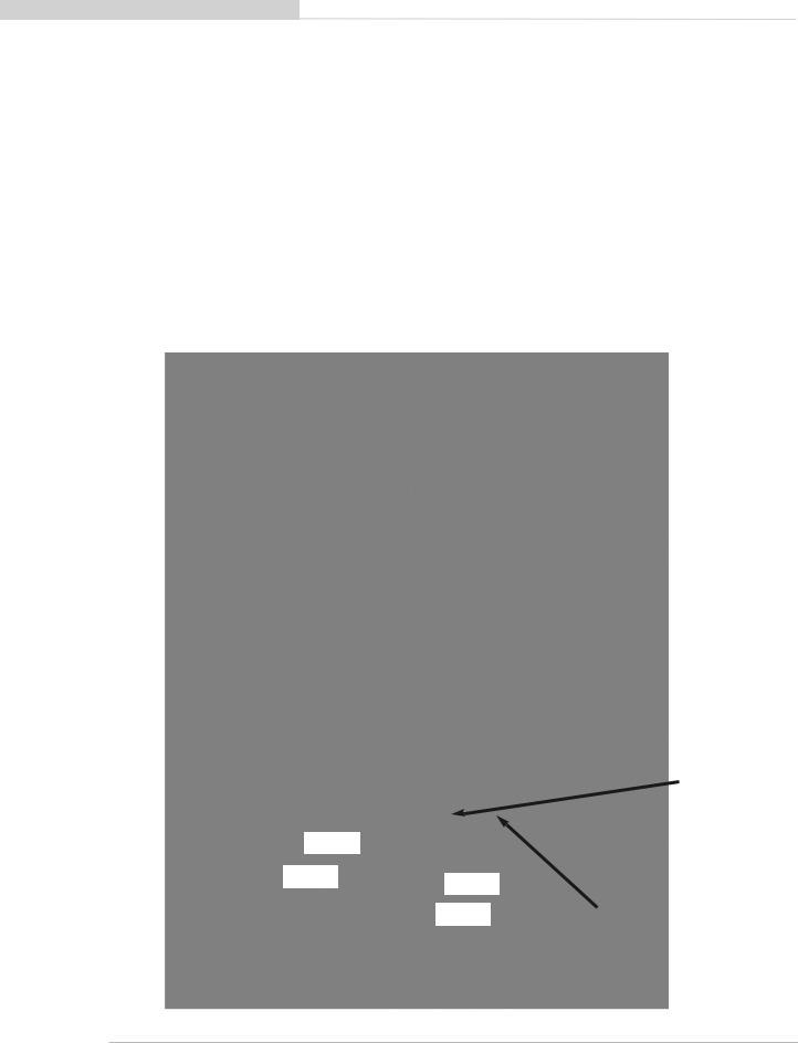
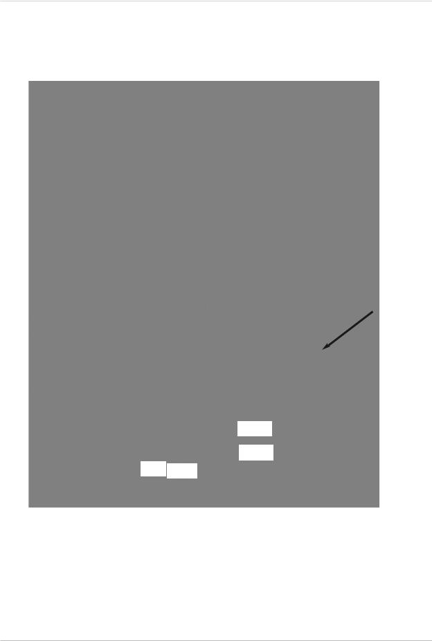
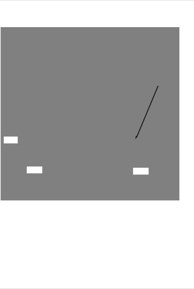
The following diagram shows the HFOV from the top view of the sensor.

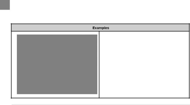
Examples

Case 1: FOV 0° to 360°

FOV command: #HDLFOV000360$

Case 2: FOV 0° to 90°

FOV command: #HDLFOV000090$

Case 3: FOV -90° to 90°

FOV command: #HDLFOV270090$

Top view of Sensor

[ 10 ]