Siemens 2005C User Manual

SOMATOM

Spirit

Application Guide

Protocols

Principles

Helpful Hints

syngo 3D

syngo Fly Through syngo Dental CT syngo Osteo CT

syngo Volume Evaluation syngo Dynamic Evaluation

Software Version syngo CT 2005C

The information presented in this Application Guide is for illustration only and is not intended to be relied upon by the reader for instruction as to the practice of medicine. Any health care practitioner reading this information is reminded that they must use their own learning, training and expertise in dealing with their individual patients.

This material does not substitute for that duty and is not intended by Siemens Medical Solutions Inc., to be used for any purpose in that regard. The drugs and doses mentioned are consistent with the approval labeling for uses and/or indications of the drug. The treating physician bears the sole responsibility for the diagnosis and treatment of patients, including drugs and doses prescribed in connection with such use. The Operating Instructions must always be strictly followed when operating the CT System. The source for the technical data is the corresponding data sheets.

The pertaining operating instructions must always be strictly followed when operating the SOMATOM Spirit. The statutory source for the technical data are the corresponding data sheets.

We express our sincere gratitude to the many customers who contributed valuable input.

Special thanks to Heike Theessen, Christiane Bredenhöller, Kristin Pacheco, Karin Ladenburger, and Chen Mahao for their valuable assistance.

To improve future versions of this Application Guide, we would greatly appreciate your questions, suggestions and comments.

Please contact us:

USC-Hotline:

Tel. no.+49-1803-112244

email [e-mail]

Editor: Ute Feuerlein

2

Overview

	User Documentation	14
	Scan and Reconstruction	16
	Dose Information	28
	Workflow Information	36
	Application Information	54
	Head	70
	Neck	88
	Shoulder	94
	Thorax	98
	Abdomen	110
	Pelvis	124
	Spine	132
	Upper Extremities	146

3

	Lower Extremities	154
	Vascular	162
	Specials	176
	Children	184
	syngo 3D	240
	syngo Fly Through	258
	syngo Dental CT	268
	syngo Osteo CT	274
	syngo Volume Evaluation	288
	syngo Dynamic Evaluation	306

4

5

Contents

	User Documentation		14
	Scan and Reconstruction		16
	• Concept of Scan Protocols		16
	• Scan Set Up		17
	• Scan Modes		18
-		Sequential Scanning	18
-		Spiral Scanning	18
-		Dynamic Serioscan	18
	• Slice Collimation and Slice Width		19
	- Slice Collimation and Slice Width for
		Spiral Mode and HR Spiral Mode	20
	- Slice Collimation and Slice Width for
		Sequence Mode and HR Sequence Mode	20
	• Increment		21
	• Pitch		22
	• Window values		23
	• Kernels		24
	• Image Filters		25
	• Improved Head Imaging		27
	Dose Information		28
	• CTDIW and CTDIVol		28
	• Effective mAs		30
	• CARE Dose		32
	- How does CARE Dose work?		32
	Workflow Information		36
	• Recon Jobs		36
	• Examination Job Status		37
	• Auto Load in 3D and Post-processing
	Presets		38
	• How to Create your own
	Scan Protocols		39
-		Edit/Save Scan Protocol	39
-		Scan Protocol Manager	40

6

Contents

	• Contrast Medium		45
-		The Basics	45
-		IV Injection	47
-		Bolus Tracking	48
-		Test Bolus using CARE Bolus	50
-		Test Bolus	51
	Application Information		54
	• SOMATOM life		54
-		General Information	54
-		Key Features	55
-		Description	56
-		Access to Computer Based Training or
		Manuals on CD ROM	57
-		SRS Based Services	58
-		Download of Files	59
-		Contact incl. DICOM Images	60
-		Trial Order and Installation	62
	• Image Converter		64
	• File Browser		66
	• Patient Protocol		68
	Head		70
	• Overview		70
	• Hints in General		71
-		Head Kernels	71
	• HeadRoutine		72
	• HeadSeq		74
	• InnerEarHR		76
	• InnerEarHRSeq		78
	• Sinus		80
	• SinusSeq		82
	• Orbita		84
	• Dental		86

7

Contents

	Neck	88
	• Overview	88
	• Hints in General	89
	- Body Kernels	90
	• Neck	92
	Shoulder	94
	• Overview	94
	• Hints in General	95
	- Body Kernels	95
	• Shoulder	96
	Thorax	98
	• Overview	98
	• Hints in General	99
	- Body Kernels	101
	• ThoraxRoutine/ThoraxRoutine08s	102
	• ThoraxFast	104
	• ThoraxHRSeq	106
	• LungLowDose	108
	Abdomen	110
	• Overview	110
	• Hints in General	111
	- Body Kernels	113
	• AbdomenRoutine/AbdomenRoutine08s	114
	• AbdomenFast	116
	• AbdMultiPhase/AbdMultiPhase08s	118
	• AbdomenSeq	122

8

Contents

	Pelvis	124
	• Overview	124
	• Hints in General	125
	- Body Kernels	125
	• Pelvis	126
	• Hip	128
	• SI_Joints	130
	Spine	132
	• Overview	132
	• Hints in General	133
	- Body Kernels	135
	• C-Spine	136
	• C-SpineSeq	138
	• Spine	140
	• SpineSeq	142
	• Osteo	144
	Upper Extremities	146
	• Overview	146
	• Hints in General	147
	- Body Kernels	148
	• WristHR	150
	• ExtrRoutineHR	152
	Lower Extremities	154
	• Overview	154
	• Hints in General	155
	- Body Kernels	156
	• KneeHR	158
	• FootHR	160
	• ExtrRoutineHR	161

9

Contents

	Vascular		162
	• Overview		162
	• Hints in General		163
-		Head Kernels	163
-		Body Kernels	163
	• HeadAngio/HeadAngio08s		164
	• CarotidAngio/CarotidAngio08s		166
	• ThorAngio/ThorAngio08s		168
	• Embolism		170
	• BodyAngioRoutine/BodyAngioRoutine08s 172
	• BodyAngioFast		174
	Specials		176
	• Overview		176
-		Trauma	176
-		Interventional CT	176
-		Test Bolus	176
	• Trauma		177
-		The Basics	177
	• PolyTrauma		178
	• HeadTrauma		180
	• Interventional CT		181
	• Biopsy		182
	• TestBolus		183
	Children		184
	• Overview		184
	• Hints in General		187
-		Head Kernels	190
-		Body Kernels	191
	• HeadRoutine_Baby		192
	• HeadRoutine_Child		194
	• HeadSeq_Baby		196
	• HeadSeq_Child		198
	• InnerEar		200
	• SinusOrbi		202
	• Neck		204

10

Contents

	• ThoraxRoutine_Baby		206
	• ThoraxRoutine_Child		208
	• ThoraxHRSeq_Baby		210
	• ThoraxHRSeq_Child		212
	• Abdomen_Baby		214
	• Abdomen_Child		216
	• Spine_Baby		218
	• Spine_Child		220
	• ExtrHR_Baby		222
	• ExtrHR_Child		224
	• HeadAngio		226
	• HeadAngio08s		228
	• CarotidAngio		230
	• CarotidAngio08s		232
	• BodyAngio		234
	• BodyAngio08s		236
	• NeonateBody		238
	syngo 3D		240
	- Multi Planar Reconstruction (MPR)		240
	- Maximum Intensity Projection (MIP)		240
	- Shaded Surface Display (SSD)		241
	- Volume Rendering Technique (VRT)		241
-		Prerequisites	242
	• Workflow		242
-		Loading the Images	242
-		Creating Series	244
-		Editing	246
-		Documentation of Results	249
	• Workflow for a CT Extremity Examination		250
-		Using MPR/MPR Thick	250
-		Using SSD	251
-		Using VRT	251
	• Workflow for a CT Angiography		252
-		Using MIP/MIP Thin	252
-		Using VRT/VRT Thin/Clip	253
	• Hints in General		254
	- Setting Views in the Volume Data Set		254
	- Changing /Creating VRT Presets		255

11

Contents

	- Auto Load in 3D and Post-processing
		Presets	257
-		Blow-up Mode	257
	syngo Fly Through		258
	• Key Features		258
	• Prerequisites		259
	• The Basics for CT Virtual Endoscopy		259
	- SSD and VRT Presets for Endoscopic
		Renderings	259
-		Endoscopic Viewing Parameters/
		Fly Cone Settings	260
-		Patient Preparation	262
	• Workflow		263
	- Navigation of the Endoscopic Volume		265
-		Fly Path Planning	266
	syngo Dental CT		268
	• The Basics		268
	• Scan Protocols		269
	• Additional Important Information		271
	syngo Osteo CT		274
	• The Basics		274
	• Scanning Procedure		275
	• Configuration		278
	• Evaluation Workflow		282
	• Additional Important Information		287
	syngo Volume Evaluation		288
	• Prerequisites		290
	• Workflow		291
	• General Hints		300
	• Configuration		303

12

Contents

	syngo Dynamic Evaluation		306
	• Prerequisites		308
	• Workflow		309
	- 1. Loading the Images		309
	- 2. Inspecting the Input Images		310
- 3.		Generation of Parameter Images	310
- 4.		Creating a Baseline Image	313
- 5.		Evaluation of Region of Interests	314
	- 6. Enhancement Curve		315
- 7.		Documentation of Results	316
	• General Hints		317

13

User Documentation

For further information about the basic operation, please refer to the corresponding syngo CT Operator Manual:

syngo CT Operator Manual Volume 1:

Security Package

Basics

Preparations

Examination

CARE Bolus CT

syngo CT Operator Manual Volume 2:

syngo Patient Browser syngo Viewing

syngo Filming syngo 3D

syngo CT Operator Manual Volume 3:

syngo Data Set Conversion syngo Dental CT

syngo Dynamic Evaluation syngo Osteo CT

syngo Volume

14

User Documentation

15

Scan and Reconstruction

Concept of Scan Protocols

The scan protocols for adult and children are defined according to body regions – Head, Neck, Shoulder,

Thorax, Abdomen, Pelvis, Spine, Upper Extremities, Lower Extremities, Specials, and Vascular.

The general concept is as follows: All protocols without suffix are standard spiral modes. E.g., “Shoulder” means the spiral mode for the shoulder.

The suffixes of the protocol name are follows:

“Routine“: for routine studies

“Seq”: for sequence studies

“Fast“: use a higher pitch for fast acquisition

“HR“: use a thinner slice width (1.0 mm) for High Resolution studies and a thicker slice width for soft tissue studies

The availability of scan protocols depends on the system configuration.

16

Scan and Reconstruction

Scan Set Up

Scans can be simply set up by selecting a predefined examination protocol. To repeat any mode, just click the chronicle with the right mouse button for “repeat”. To delete it, select “cut“. Each range name in the chronicle can be easily changed before “load“.

Multiple ranges can be run either automatically with “auto range“, which is denoted by a bracket connecting the two ranges, or separately with a “pause” in between.

17

Scan and Reconstruction

Scan Modes

Sequential Scanning

This is an incremental, slice-by-slice imaging mode in which there is no table movement during data acquisition. A minimum interscan delay in between each acquisition is required to move the table to the next slice position.

Spiral Scanning

Spiral scanning is a continuous volume imaging mode. The data acquisition and table movements are performed simultaneously for the entire scan duration. There is no interscan delay and a typical range can be acquired in a single breath hold.

Each acquisition provides a complete volume data set, from which images with overlapping can be reconstructed at any arbitrary slice position. Unlike the sequence mode, spiral scanning does not require additional radiation to obtain overlapping slices.

Dynamic Serioscan

Dynamic serial scanning mode without table feed. Dynamic serio can still be used for dynamic evaluation, such as Test Bolus.

18

Scan and Reconstruction

Slice Collimation and

Slice Width

Slice collimation is the slice thickness resulting from the effect of the tube-side collimator and the adaptive detector array design. In Multislice CT, the Z-coverage per rotation is given by the product of the number of active detector slices and the collimation (e.g., 2 x 1.0 mm).

Slice width is the FWHM (full width at half maximum) of the reconstructed image.

With the SOMATOM Spirit, you select the slice collimation together with the slice width desired. The slice width is independent of pitch, i.e. what you select is always what you get. Actually, you do not need to be concerned about the algorithm any more; the software does it for you.

The Recon icon on the chronicle will be labeled with “RT”. After the scan, the Real Time displayed image series has to be reconstructed.

The following tables show the possibilities of image reconstruction in spiral and sequential scanning.

19

Scan and Reconstruction

Slice Collimation and Slice Width for Spiral Mode and HR Spiral Mode

1 mm:	1, 1.25, 2, 3, 5 mm
1.5 mm:	2, 3, 5, 6 mm
2.5 mm:	3, 5, 6, 8, 10 mm
4 mm:	5, 6, 8, 10 mm
5 mm:	6, 8, 10 mm

Slice Collimation and Slice Width for Sequence Mode and HR Sequence Mode

1.0 mm:	1, 2 mm
1.5 mm:	1.5, 3 mm
2.5 mm:	2.5, 5 mm
4.0 mm:	4,	8 mm
5.0 mm	5,	10 mm

20

Scan and Reconstruction

Increment

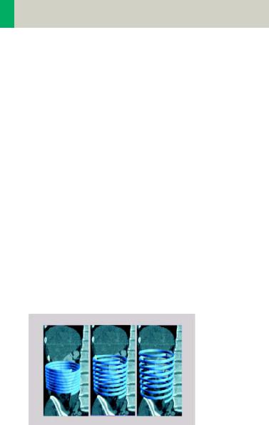
The increment is the distance between the reconstructed images in the Z direction. When the increment chosen is smaller than the slice thickness, the images are created with an overlap. This technique is useful to reduce partial volume effect, giving you better detail of the anatomy and high quality 2D and 3D post-process- ing.

Slice Thickness = 10 mm

	Increment = 3 mm
Increment = 10 mm	Increment = 5 mm

Reconstruction Increment

21

Scan and Reconstruction

Pitch

In single slice CT:

Pitch = table movement per rotation/slice collimation

E.g.,: slice collimation = 5 mm,

table moves 5 mm per rotation, then pitch = 1.

With the Siemens Multislice CT, we differentiate between:

Feed/Rotation, the table movement per rotation

Volume Pitch, table movement per rotation/single slice collimation.

Pitch Factor, table movement per rotation/complete slice collimation.

E.g., slice collimation = 2 x 5 mm, table moves 10 mm per rotation,

then Volume Pitch = 2, Pitch Factor = 1.

With the SOMATOM Spirit, the pitch, slice, collimation, rotation time, and scan range can be adjusted. The pitch factor can be selected from 0.5-2.

Pitch 1

Pitch 1.5

Pitch 2

Pitch Models

22

Scan and Reconstruction

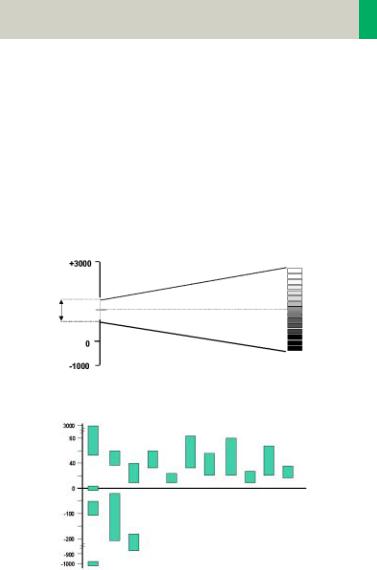
Window values

The Scale of the CT Hounsfield Units is from -1024 to +3071.

The displayed window values have to correspond to the anatomical structure.

Windowing is used to optimize contrast and brightness of images.

Hounsfield Units			Gray scale
			white
Window	Window
width W	center C
			black
		CT-window values
	Blood	Liver
Spleen Kidneys		Tumor
		Heart
Bones	Pancreas Adrenal	Colon	Bladder
	Glands

Water

Breast

Fat

Air Lung

Organ specific window values

23

Scan and Reconstruction

Kernels

There are 3 different types of kernels: “H“ stands for Head, “B“ stands for Body, “C“ stands for ChildHead.

The image sharpness is defined by the numbers – the higher the number, the sharper the image; the lower the number, the smoother the image.

A set of 18 kernels is supplied, consisting of:

•6 body kernels: smooth (B20s), medium smooth (B31s), medium (B41s), medium sharp (B50s), sharp (B60s), high res (B70s)

•7 head kernels: smooth (H21s), medium smooth (H31s), medium (H41s), medium sharp (H50s), sharp (H60s), high res (H70s), ultra high res (H80s)

•3 child head kernels: smooth (C20s), medium (C30s), sharp (C60s)

•2 special kernels: S80s, U90s

Note: Do not use different kernels for body parts other than what they are designed for.

For further information regarding the kernels, please refer to the “Hints in General” of the corresponding body region.

24

Scan and Reconstruction

Image Filters

There are 3 different filters available:

LCE: The Low-contrast enhancement (LCE) filter enhances low-contrast detectability. It reduces the image noise.

•Similar to reconstruction with a smoother kernel

•Reduces noise

•Enhances low-contrast detectability

•Adjustable in four steps

•Automatic post-processing

25

Scan and Reconstruction

HCE: The High-contrast enhancement (HCE) filter enhances high-contrast detectability. It increases the image sharpness, similar to reconstruction with a sharper kernel.

•Increases sharpness

•Faster than raw-data reconstruction

•Enhances high-contrast detectability

•Automatic post-processing

ASA: The Advanced Smoothing Algorithm (ASA) filter reduces noise in soft tissue, while edges with high contrast are preserved.

•Reduces noise without blurring of edges

•Enhances low-contrast detectability

•Individually adaptable

•Automatic post-processing

26

Scan and Reconstruction

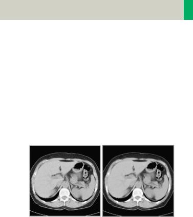
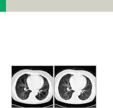
Improved Head Imaging

An automatic bone correction algorithm has been included in the standard image reconstruction. Using a new iterative technique, typical artifacts arising from the beam-hardening effect, e.g., Hounsfield bar, are minimized without any additional post-processing. This advanced algorithm allows for excellent images of the posterior fossa, but also improves head image quality in general. Bone correction is activated automatically for body region “Head”.

In order to optimize image quality versus radiation dose, scans in the body region “Head” are provided within a maximum scan field of 300 mm with respect to the iso-center. No recon job with a field of view exceeding those limits will be possible. Therefore, patient positioning has to be performed accurately to ensure a centered location of the skull.

Head image without correction.

Head image with corrections.

27

Dose Information

CTDIW and CTDIVol

The average dose in the scan plane is best described by the CTDIW for the selected scan parameters. The CTDIW is measured in the dedicated plastic phantoms – 16 cm diameter for head and 32 cm diameter for body (as defined in IEC 60601 –2 – 44). This dose number gives a good estimate for the average dose applied in the scanned volume as long as the patient size is similar to the size of the respective dose phantoms.

Since the body size can be smaller or larger than

32 cm, the CTDIW value displayed can deviate from the dose in the scanned volume.

The CTDIW definition and measurement is based on single axial scan modes. For clinical scanning, i.e. scanning of entire volumes in patients, the average dose will also depend on the table feed in between axial scans or the feed per rotation in spiral scanning. The dose, expressed as the CTDIW, must therefore be corrected by the Pitch Factor of the spiral scan or an axial scan series to describe the average dose in the scanned volume.

For this purpose the IEC defined the term “CTDIVol“ in September 2002:

CTDIVol = CTDIW/Pitch Factor

This dose number is displayed on the user interface for the selected scan parameters.

28

Dose Information

The CTDIvol value does not provide the entire information of the radiation risk associated with CT examination. For the purpose, the concept of the “Effective Dose“ was introduced by ICRP (International Commission on Radiation Protection). The effective dose is expressed as a weighted sum of the dose applied not only to the organs in the scanned range, but also to the rest of the body. It could be measured in whole body phantoms (Alderson phantom) or simulated with Monte Carlo techniques.

The calculation of the effective dose is rather complicated and has to be done by sophisticated programs. These have to take into account the scan parameters, the system design of individual scanner, such as x-ray filtration and gantry geometry, the scan range, the organs involved in the scanned range and the organs affected by scattered radiation. For each organ, the respective dose delivered during the CT scanning has to be calculated and then multiplied by its radiation risk factor. Finally, the weighted organ dose numbers are added up to get the effective dose.

The concept of effective dose allows the comparison of radiation risk associated with different CT or x-ray exams, i.e. different exams associated with the same effective dose would have the same radiation risk for the patient. It also allows comparing the applied x-ray exposure to the natural background radiation,

e.g., 2 – 3 mSv per year in Germany.

29

Dose Information

Effective mAs

In sequential scanning, the dose (Dseq) applied to the patient is the product of the tube current-time (mAs) and the CTDIw per mAs:

Dseq = DCTDIw x mAs

In spiral scanning, however, the applied dose (Dspiral) is influenced by the “classical“ mAs (mA x Rot Time) and in addition by the Pitch Factor. For example, if a Multislice CT scanner is used, the actual dose applied to the patient in spiral scanning will be decreased when the Pitch Factor is larger than 1, and increased when the Pitch Factor is smaller than 1. Therefore, the dose in spiral scanning has to be corrected by the Pitch Factor:

Dspiral = (DCTDIw x mA x Rot Time)/Pitch Factor

To make it easier for the users, the concept of the “effective“ mAs was introduced with the SOMATOM Multislice scanners.

The effective mAs takes into account the influence of pitch on both the image quality and dose:

Effective mAs = mAs/Pitch Factor

To calculate the dose you simply have to multiply the CTDIw per mAs with the effective mAs of the scan:

Dspiral = DCTDIw x effective mAs

30