PASCO Xplorer-GLX User Manual

Users’ Guide

•Using the Xplorer GLX Standalone

•Using the Xplorer GLX with a Computer

•Sample Activities

New Features:

•File storage on USB flash drive, p. 83

•Update firmware from flash drive, p. 93

•Instant data monitoring in Digits and Meter displays, pp. 37 & 38

•Voice and Text Data Annotation, p. 25

(more on page ii)

01208950F

ii

About this Guide

The Xplorer GLX Users’ Guide is divided into two parts.

Part 1 contains detailed information about operating the GLX, including descriptions of every screen, window and menu within the GLX environment, and instructions for common procedures.

Part 2 contains step-by-step instructions for science activities and experiments that can be done with the GLX, its standard included equipment, and commonly available supplies.

This is revision F of the User’s Guide, for version 1.4x of the GLX firmware. Visit www.PASCO.com/glx/ for downloadable updates to the Users’s Guide and firmware. If you have updated your GLX from a previous version, be sure to check out these new features:

New for Version 1.4x	Update firmware from USB flash drive, p. 93
	Cell-selective manual sampling with Table display, p. 60
	Instant data monitoring in Digits and Meter displays, pp. 37 & 38
	Automatic calculation creation from Linear Fit, p. 22
	Export data to text file, p. 32
New for Version 1.3x	Swap Cursors, p. 21
	Toggle Active Data, p. 21
	Zoom Tool, p. 25
New for Version 1.2x	Voice and Text Data Annotation, p. 25
	USB flash drive support, p. 83
	GLX-to-GLX data transfer, p, 84
New for Version 1.1x	Scope Mode, p. 22
	Output-control Calculations, p. 50
	Built-in Sound Sensor, p. 58
	Data Collection with ScienceWorkshop Sensors pp. 59, 67

Technical Support

For assistance with the Xplorer GLX and other PASCO products, contact PASCO Technical Support at:

Address:	PASCO scientific
	10101 Foothills Blvd.
	Roseville, CA, 95747-7100 USA
Phone:	(800)	772-8700 (in the U.S.)
	(916)	786-3800 (worldwide)
Fax:	(916)	786-7565
Web:	www.pasco.com/support/
Email:	[e-mail]

Copyright

The PASCO scientific Xplorer GLX Users’ Guide is copyrighted with all rights reserved. Permission is granted to non-profit educational institutions for reproduction of any part of this manual, providing the reproductions are used only in their laboratories and classrooms, and are not sold for profit. Reproduction under any other circumstances, without the written consent of PASCO scientific, is prohibited.

Trademarks

PASCO, PASCO scientific, DataStudio, PASPORT, ScienceWorkshop, Xplorer, and Xplorer GLX are trademarks or registered trademarks of PASCO scientific, in the United States and/or in other countries. All other brands, products, or service names are or may be trademarks or service marks of, and are used to identify products or services of, their respective owners. For more information visit www.pasco.com/legal.

Windows is a registered trademark of Microsoft Corporation in the United States and/or other countries.

Macintosh, Mac, and Mac OS are trademarks of Apple Computer, Inc., registered in the U.S. and other countries.

PASCO Manual Number 012-08950F

ä

How to Store the

Even when the screen is blank, the GLX is active: it powers its memory, it periodically checks its battery, and it monitors its keypad. Like other hand-held computers, the GLX never turns off—it just goes to sleep.

Before you put your GLX away, read these instructions.

With proper care, you can ensure that your GLX will be ready for use whenever you need it.

Storage Time What You Should Do

WHENEVER	Leave the GLX Plugged In
POSSIBLE	Leave the GLX connected to AC power so it can keep its battery charged and store data
	files indefinitely. This is the best way to store the GLX for any length of time.
Unplugged for
MORE THAN	Backup Your Data
A FEW DAYS	Data files stored in RAM are temporary. If you want to keep your data files, transfer them to
	the GLX's internal Flash memory, a USB Flash drive, or a computer. See pages 78–84 and
	100 of the Users' Guide for more information.
	Fully Charge the Battery
	Put the GLX away with a full battery to keep the RAM active (for up to two weeks) and
	ensure that the battery has power the next time you use it.
	Any time within two weeks, simply press and hold the power button to turn it on. Data
	saved in RAM will still be there.
	After two weeks, plug in the AC adapter to turn on the GLX (or press the reset button on
	the back) and retrieve data files from your backup location.

Unplugged for

MORE THAN Put the GLX into Deep Sleep*
A MONTH	In deep sleep mode, an internal switch opens to disconnect the battery. To put the GLX
	into deep sleep: backup your data; allow the battery to fully charge; unplug the AC adapter;
	go to the settings screen, press F3 , and press	; follow the on-screen instructions.

Why is deep sleep important?

Nickel metal hydride batteries last longer when they are kept as fully charged as possible. Deep sleep mode prevents unnecessary discharging.

What if I forget to put it into deep sleep?

Don't worry. If the GLX is left unplugged and unused from more than two weeks, it puts itself into deep sleep.

How do I wake up the GLX from deep sleep?

When you're ready to use it again, just plug in the AC adapter (or press the reset button on the back) and retrieve data files from your backup location.

*Note for early hardware versions: Early versions of the GLX do not support deep sleep mode. If you have one of these GLXs, leave it plugged in or remove the battery for long-term storage. (But don't plug in the AC adapter when the battery in not installed.) See page 95 of the Users' Guide for more information.

TAPE THIS SHEET TO THE INSIDE LID OF THE GLX STORAGE BOX OR POST IT WHERE THE GLX WILL BE STORED.

®

Visit www.pasco.com/glx to download the latest GLX firmware update and Users’ Guide.012-08950F

Contents

Part 1:
Users’ Guide
Introduction . . . . . . . . . . . . . . . . . . . . . .	. 3
Included Equipment . . . . . . . . . . . . . . . .	4
Quick Start . . . . . . . . . . . . . . . . . . . . . . .	5
Overview of the GLX . . . . . . . . . . . . . . . .	6
Chapter 1: Displays
Graph . . . . . . . . . . . . . . . . . . . . . . . . . .	13
Table . . . . . . . . . . . . . . . . . . . . . . . . . . .	28
Digits Display . . . . . . . . . . . . . . . . . . . .	37
Meter . . . . . . . . . . . . . . . . . . . . . . . . . . .	38

Chapter 2: Utility Screens

Output . . . . . . . . . . . . . . . . . . . . . . . . . . 39

Calculator . . . . . . . . . . . . . . . . . . . . . . . 41

Notes Screen . . . . . . . . . . . . . . . . . . . . 53

Stopwatch . . . . . . . . . . . . . . . . . . . . . . . 54

Chapter 3: Settings and Files
Sensors Screen . . . . . . . . . . . . . . . . . .	55
Timing Screen . . . . . . . . . . . . . . . . . . . .	62
Data Properties . . . . . . . . . . . . . . . . . . .	69
Calibration . . . . . . . . . . . . . . . . . . . . . . .	71
Data Files Screen . . . . . . . . . . . . . . . . .	78
Settings Screen . . . . . . . . . . . . . . . . . . .	85
Chapter 4: Navigation and Input
Data Source Menus . . . . . . . . . . . . . . .	89
Multipress Text Input Mode . . . . . . . . . .	90
Using a USB Keyboard . . . . . . . . . . . . .	90
Scientific Notation . . . . . . . . . . . . . . . . .	91
Printing . . . . . . . . . . . . . . . . . . . . . . . . .	91

Chapter 5: Hardware Maintenance and

Operation
Firmware Update . . . . . . . . . . . . . . . .	. 93
Battery and Power . . . . . . . . . . . . . . .	. 93
Resetting . . . . . . . . . . . . . . . . . . . . . .	. 96
Operating Temperature . . . . . . . . . . . .	97
Chapter 6: Using the Xplorer GLX
with a Computer
GLX with DataStudio . . . . . . . . . . . . . .	99
GLX Simulator . . . . . . . . . . . . . . . . . .	103

Part 2:

Sample Activities

Activity 1: Calorimetry . . . . . . . . . . . . . 107 Activity 2: Melting Point Depression. . . 111 Activity 3: Heat Transfer by Radiation . 113 Activity 4: Newton’s Law of Cooling . . . 115 Activity 5: Microclimate Temperature

Variation. . . . . . . . . . . . . . . . 121 Activity 6: Voltage versus Resistance . 123 Activity 7: Induced Electromotive Force 127 Activity 8: Capacitor Discharge . . . . . . 131 Activity 9: Constructive and Destructive

Interference . . . . . . . . . . . . . 135 Activity 10: Beat Frequency . . . . . . . . . . 137

Index	141
Shortcut Summary	143

Part 1:

Users’ Guide

X p l o r e r G L X U s e r s ’ G u i d e

3

Introduction

The Xplorer GLX is a data collection, graphing, and analysis tool designed for science students and educators. The Xplorer GLX supports up to four PASPORT sensors simultaneously, in addition to two temperature probes and a voltage probe connected directly to specialized ports.

An optional mouse, keyboard, or printer can be connected to the Xplorer GLX’s USB ports. The Xplorer GLX contains an integrated speaker for sound generation and a stereo signal output port for optional headphones or amplified speakers.

The Xplorer GLX is fully functional stand-alone handheld computing device for science. It also operates as PASPORT sensor interface when connected to a desktop or laptop computer running DataStudio software.

4	I n c l u d e d E q u i p m e n t

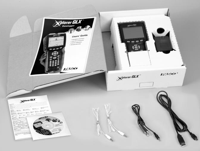
Included Equipment

A B C

D

E F G H

A)	GLX Users’ Guide	F)	Two Fast-response Temperature Probes
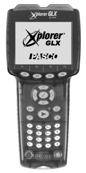
B)	Xplorer GLX		(-10 to 70 °C)
C)	AC Power Adapter	G)	Voltage Probe (-10 to +10 V)
D)	Registration Card	H)	USB Host-connection Cable
E)	Getting Started with the Xplorer GLX CD-ROM	I)	Poster (not pictured)

X p l o r e r G L X U s e r s ’ G u i d e

5

Quick Start

Getting started with the GLX is easy—simply plug in the AC adapter, connect one of the included sensors, and collect data. In the example below, you will start the GLX and collect temperature data.

1. Plug In the AC Adapter

Connect the AC adapter to the power port on the right side of the GLX and plug the adapter into a power outlet (100 to 240 VAC, depending on your location). When you connect the AC adapter, the GLX turns on automatically.

The first time you use the GLX, leave it plugged in overnight (at least 14 hours) to allow the battery to fully charge.

If the battery has already been charged, you can use the GLX without the AC adapter. To turn it on using battery power, push the power button at the lowerright corner of the keypad ( ) and hold it for about one second.

2. Connect a Sensor

Connect a temperature probe to one of the temperature ports on the left side of the GLX.

In most cases, the Graph display will launch automatically with the axes labeled “Temperature (°C)” and “Time (s).”

Connect the AC power adapter

If running on battery power, press the power button

Connect a temperature probe

3. Collect Data

Press .

The GLX is now recording and graphing data from the sensor. Press F1 to automatically scale the graph.

Hold the end of the temperature probe in your hand and observe how the data plotted on the Graph react.

6	O v e r v i e w o f t h e G L X

To stop data recording, press again.

You have just collected and graphed a run of temperature data. To collect additional data runs, press again.

There are several different ways to collect data with the GLX. This is the simplest and most common. See “F1 Mode” on page 57 for other options. You can find a complete description of the Graph display starting on page 13.

Overview of the GLX

The example above represents just a small part of the GLX’s capabilities. This overview will outline some of the set-up options to customize your GLX and prepare it for an activity; then (starting on page 9) survey the GLX’s Home Screen as a gateway to the entire GLX environment.

Equipment Set-up Options

Power Source Whenever possible, it is a good idea to use the GLX connected to the AC power supply. For maximum operating time on battery power, first connect the GLX to AC power for at least 14 hours, or until the Battery Gauge indicates a full charge.1

Power On The power turns on automatically when you plug in the AC adapter. If the GLX is running on batteries, or if the AC adapter is already connected, push and hold the power button ( ) for about 1 second to turn it on.

By default, the GLX is set to start with a new data file; however, if the Startup Action of the GLX has been set to “Open Last Experiment,” it will automatically open the most recently saved file. See page 86 for more information.

Back Light To turn on the screen’s back light, press and hold while you press .2

Screen Contrast There are 21 levels of screen contrast. Push and hold , then use the up and down arrow keys ( ) to adjust the contrast to a comfortable level.

Language In its factory configuration, the GLX is set up to operate in English. If you would like to change the language, refer to “Settings Screen” on page 85.

PASPORT Sensors Connect up to four PASPORT sensors to the main ports on top of the GLX.

In some cases, the GLX may automatically launch the Graph or other display when you plug in a sensor. See “Sensor Auto-Display” on page 86 for more information about this feature.

Temperature Probes Connect the included fast-response probes or other PASCO temperature probes to the two temperature ports on the left side of the GLX. The range is -10 to +70 °C with fast-response probes, or -10 to +135 °C with stainless steel probes.

Voltage Probe Connect the included voltage probe to the voltage port on the left side of the GLX to measure voltages between -10 and +10 V. The voltage probe should be connected to voltage sources only when it is also connected to

1See “Battery Gauge” on page 11.

2The backlight and other aspects of the Xplorer GLX can also be adjusted in the Settings Screen. See page 85.

Temperature Signal

Probes Output

Security Cable

Connection Slot

Voltage

Probe

PASPORT

Sensor Ports

X p l o r e r G L X U s e r s ’ G u i d e

7

the GLX. Do not connect a voltage source until after the probe is connected to the GLX; remove any voltage sources before disconnecting the probe.

Sound Sensor To configure the GLX’s microphone as a sound sensor, press and F4 together to enter the Sensors screen; then press F3 to open the

Microphone menu. From the menu, select Sound Sensor to record the sound waveforms, or select Sound Level to measure sound level in decibels. See “F3 Microphone” on page 58 for more information.

Computer If you will be using the GLX with a computer, use the included USB host-connection cable to connect the GLX to the USB port of the computer. Refer to page 99 for instructions on setting up the computer.

Mouse If you will be using an optional mouse (PS-2539), connect it to the USB port on the right side of the GLX.

A mouse can be convenient, but it is never required; anything that you can do with the mouse can also be done through the GLX’s keypad. New users often find that operating the GLX is easier with a mouse. For experienced users, using the keypad rather than a mouse is usually faster.

Keyboard If you plan to do a lot of text entry, connect a USB keyboard (PS-2541) to the port on the right side of the GLX.

To connect a mouse and a keyboard simultaneously, use the optional

PS-2536 Peripheral Cable.

Signal Output If you have headphones or a pair of amplified stereo speakers that you wish to use for sound generation, connect them to the signal output port. You also have the option of using the GLX’s built-in speaker for sound output. See “Output” on page 39 for more information.

USB Storage Device If you have a USB storage device (such as a flash drive) you can connect it to the GLX’s USB port for extra file-storage capacity and data backup. See page 83 for more information.

GLX-to-GLX Transfer If you have two GLXs that you would like to transfer files between, connect them using the included host-connection cable. See page 84 for more information.

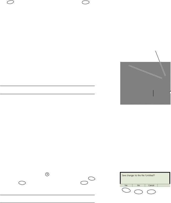
Shutting Down

Manual Shut Down

To turn off the GLX, press and hold	for 1 second. The GLX will prompt you
to save your data and experiment setup before it shuts down. Press			F1 to save
your work, press F2 to shut down without saving, or press		F3	to not shut
down. See page 80 for instructions on opening the saved file.

If you hold the power button for 5 seconds, the GLX will shut down without saving your data.

The GLX cannot shut down while the battery is charging; if you try to turn it off, a message will appear informing you that charging is in progress. When the battery is fully charged, and the GLX has been idle for 60 minutes, it will shut down automatically (see below).

Computer via USB host-connection cable or

Mouse, keyboard or printer through optional peripheral cable

USB mouse, keyboard, printer, storage device, or 2nd GLX

AC power adapter

F1	F2	F3

8	O v e r v i e w o f t h e G L X

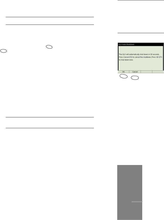
Auto Power Off

Timed Auto Power Off If it is running on battery power, the GLX will automatically save your data and shut down after a certain amount of continuous idle time (5 minutes by default).3

To set the idle time that must elapse before auto shut down on battery power, see “Auto Power Off” on page 85.

If the GLX is running on AC power and the battery is fully charged, it will automatically shut down after 60 minutes of idle time.

The GLX will warn you that it is about to shut down 30 seconds before it actually does. If you see the warning, press F1 to proceed with the shutdown, or press

F2 to keep the GLX turned on.

Battery Auto Power Off The GLX will also save data and shut down automatically if the batteries drain to a critical level. Connect AC power before turning the GLX back on.

Auto Data Save Just before the GLX shuts down, it will save the open file (which includes all data, displays, calculations and set-up information). If you have named the file, it will be saved under that name. If you have not named the file, it will be saved with the filename “Untitled.”

Resuming after Auto Power Off To resume your work after the GLX automatically shuts down, push and hold the power button ( ) for about 1 second to turn it on. If the automatically saved file does not open automatically, go to the Data Files screen (see page 78) and open the file. (See page 80 for instructions on opening a file.)

If you have set the Startup Action of the GLX to “Open Last Experiment,” the file will automatically open when you turn on the GLX. See page 86 for more information.

Sleep Between Samples If the GLX is running on battery power and collecting data at a rate of once every 30 s or slower, and it has been otherwise idle for the set auto-power-off time (see page 85), it will “sleep” between samples. When the GLX is sleeping, the screen and any connected sensors are turned off to save power, and the green LED on the front of the unit blinks once every two seconds. When it is time to collect a data point, the GLX wakes up briefly, records data, and goes back to sleep. Press any key to wake up the GLX.

The Record Button

Default Recording Mode Whenever you have one or more sensors connected to the GLX, you can press to start data collection. In its default mode, the GLX will begin recording data continuously from all connected sensors. Press again to stop data collection. To start recording another data run, press yet again.

Sticky Start Use the Sticky Start feature to prevent data collection from being unintentionally stopped when you take the GLX on an amusement park ride. To start data collection with Sticky Start, press and hold for about 5 seconds.

You will hear three beeps and see the Sticky Start icon () appear at the top of the screen. Data recording will continue after you release . To stop data

3The GLX is considered idle when

•the GLX is not collecting data,

•the Stopwatch is not running,

•the GLX is not connected to a computer running DataStudio, and

•the GLX is not receiving input through its keypad, a mouse, or a USB keyboard.

F1 F2

Record Button

X p l o r e r G L X U s e r s ’ G u i d e

9

recording, you must press and hold recording will stop when you release

until you hear three beeps again. Data .

Alternative Recording Modes If you have put the GLX into Manual Sampling mode (see page 57), it will not start recording when you press ; rather it will stand by to record a data point whenever you press . If you have turned on the Trigger in the Graph display (see page 20), then the GLX will delay the start of recording after you press until the specified trigger condition is reached.

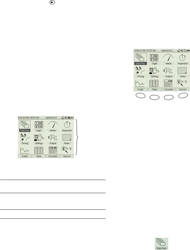
Home Screen

The Home Screen is the center of the GLX environment. All other screens are just one step away from the Home Screen. From any other screen, you can always return to the Home Screen by pressing .

The Home Screen consists of three sections: the Main Icons, the Bottom Row, and the Top Bar.

Main Icons	F1			F4
		F2	F3
The main icons on the Home Screen lead to the other screens of the GLX envi-		The Home Screen
ronment.

Main

Icons

To open another screen via one of the main icons, use the up, down, left, and right arrow keys to highlight the desired icon, then press .

The highlight wraps around, so you can move it to any icon within three key presses. For instance, if the highlight is in the first column, and you want to move it to the fourth column, press the left arrow key once.

Alternatively, if you are using a mouse, simply click on the desired icon.

You can also access the four icons in the bottom row using the function keys.

See “Bottom Row” on page 10 for more information.

The icons and the screens they lead to are described briefly here, and in more detail elsewhere in the following chapters.

Data Files Once you have collected data or configured the GLX for an experiment, you can go to the Data Files screen to save your work. You can also open or delete saved files and manage the displays, sensors, calculations, and manually entered data sets that are part of a data file. See page 78 for more information.

10	O v e r v i e w o f t h e G L X

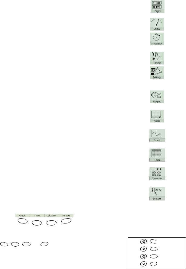
Digits This screen is useful for displaying live data as they are collected from sensors and calculations. Up to six data sources can be displayed simultaneously. See page 37 for more information.

Meter This display simulates an analog meter with a needle that deflects in proportion to a measurement made by a sensor. See page 38 for more information.

Stopwatch With this screen, the GLX can be used like a regular stopwatch to time events. The stopwatch is started and stopped by the user through the GLX’s keypad, so no sensors are necessary. See page 54 for more information.

Timing Use the Timing screen to configure photogates, Super Pulleys, and other switch-type or counting-type digital sensors. See page 62 for more information.

Settings Go to the Settings screen to change the GLX’s name, time and date, and screen settings, set how long the GLX waits before automatically turning off, and control how the GLX behaves when you turn it on or connect a sensor. See page 85 for more information.

Output The Output screen contains the controls for the signal that the GLX generates and outputs through the built-in speaker, or through the signal output port to headphones or amplified speakers. See page 39 for more information.

Notes In the Notes screen, you can create, read, and edit pages of text notes to be saved along with an experiment configuration or collected data. See page 53 for more information.

Graph Use the Graph to plot and analyze data. In many cases, the Graph is the best way to view data as they are being collected. See page 13 for more information.

Table The Table displays data numerically in columns. It can be used for editing and entering data and for statistical analysis. See page 28 for more information.

Calculator You can use the calculator like a regular calculator for finding the result of a simple expression and like a graphing calculator for plotting equations. The calculator can also perform operations on streams of data collected from sensors and on sets of manually entered data. See page 41 for more information.

Sensors Use the Sensors screen to customize the way sensors collect data. The screen shows which sensors are connected to the GLX and contains controls for how each sensor operates. See page 85 for more information.

Bottom Row

F1	F2	F3	F4

Bottom Row

The icons in the bottom row of the Home Screen are selectable via the four function keys: F1 , F2 , F3 , and F4 . Graph, Table, Calculator, and Sensors are the most commonly used screens, and therefore the most easily accessible. To make the bottom row of the Home Screen appear temporarily from anywhere in the GLX environment, press and hold ; while holding , press one of the function keys to open the corresponding screen.

In other screens, you will usually see four choices at the bottom of the screen that can be accessed with the function keys.

+ F1 Graph

+ F2 Table

+ F3 Calculator

+F4 Sensors

Shortcuts from anywhere in the GLX environment

Battery

Gauge

X p l o r e r

Top Bar

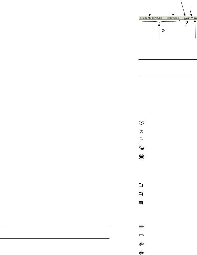
The Top Bar is the part of the Home Screen that is always visible from anywhere in the GLX environment. It shows the time and date and the name of the GLX or the name of the open file. It also indicates the recording status, battery level and memory usage.

Time and Date The time and date displayed in the Top Bar are set automatically when you connect the GLX to a computer running DataStudio (see

page 99). You can also go to the Settings screen (see page 85) to set the time and date manually and change the format in which they are displayed.4

G L X U s e r s ’ G u i d e

11

			Home
			Icon	Memory
		GLX Name		Gauge
Time and Date
		or File Name
		Recording Indicator
		when recording
		(click to start and stop)

Click to

access Settings

Top Bar

GLX Name By default, the name displayed in the Top Bar is “XplorerGLX.” If you are using more than one GLX in your classroom or lab, you may wish to give each one a unique name. See “Settings Screen” on page 85 for instructions.

When a previously saved filed is open, the name of that file appears in place of the GLX Name. See page 78 for more information about saving and opening files.

Home Icon If you are using a mouse, you can click the Home Icon () in the Top Bar, instead of pressing on the keypad, to return to the Home Screen from any other screen in the GLX environment.

Recording Status The Recording Status icon changes to indicate when the GLX is collecting data, and in what sampling mode it is operating (see page 57 for more information about the sampling modes). It also indicates when an audio note is being recorded or played (see “Data Annotation” on page 25).

If you are using a mouse, you can click the Recording Status icon, instead of pressing on the keypad, to start and stop data collection.

Memory Gauge The Memory Gauge indicates the GLX’s available memory. As data are stored in random access memory (RAM), the icon becomes shaded from the bottom up. An entirely shaded icon means that there is little or no capacity remaining for recording data. See “Data Files Screen” on page 78 for instructions on deleting files or data runs to make more memory available.

If you are using a mouse, you can click the Memory Gauge to open the Data Files screen, start a new file, or save the file that you are working with. (Without a mouse, the Data Files screen, which includes the New File and Save File options, is accessed through the Home Screen; see page 78.)

Battery Gauge When the GLX is running on battery power, the Battery Gauge indicates the level of charge of the battery. It is fully charged when the entire gauge is shaded.

Each GLX learns the particular charge and discharge characteristics of its battery as it is used. To make the gauge more accurate, allow the battery to fully charge, then fully discharge at least once.

The Battery Gauge also indicates when the GLX is connected to AC power and charging the battery.

4The time can be displayed in 12-hour or 24-hour format; the date can be displayed as month/day/year or day/month/year.

Recording Status Icons

Not Collecting Data

Sampling in Continuous Mode

Sampling in Manual Mode

Recording Audio Note

Playing Audio Note

Memory Gauge Icons

Most RAM free

RAM about half free

RAM almost full

Battery Gauge Icons

Battery fully charged

Battery nearly empty

AC power connected; battery charging

AC power connected; battery fully charged

12	O v e r v i e w o f t h e G L X

X p l o r e r G L X U s e r s ’ G u i d e

13

Chapter 1: Displays

The GLX has four screens for displaying data: Graph, Table, Digits, and Meter. This chapter will describe the structure and use of each display.

Open any of the displays to monitor live data as it is collected. Open the Graph or Table to view previously recorded measurements or manually entered data.

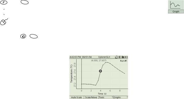
Graph

The Graph plots data on a pair of axes. Use the Graph to view, compare, and analyze data sets.

To Open the Graph

From the Home Screen, do one of the following:

press F1 , the function key below the Graph icon;

use the arrow keys to highlight the Graph icon, then press ; or

click the Graph icon.

From anywhere in the GLX environment, you can always open the Graph with

the shortcut

+ F1 .

In some cases, the Graph opens automatically when you connect a sensor.

The Graph icon on the Home Screen

The Graph Display

14 G r a p h

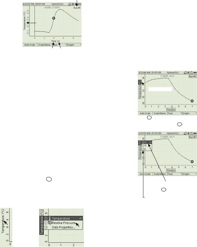
Active Fields

Run Number

Units

Data

Source

Data Source

Units

Active fields of the Graph

Active fields are the areas on the Graph (and other display screens) through which you control what data are shown. When you select an active field, a menu opens containing choices of data source, units, or run number. Follow the steps below to select an active field using the keypad.

1.Press to “light up” the active fields—shaded boxes appear around the active fields.

2.One of the shaded boxes is darker than the others, designating the highlighted field. Use the arrow keys to move the highlight to the field that you would like to select.

3.Press again to select the highlighted field, which causes a menu to open. To select an option from the menu:

•use the up and down keys to highlight the desired menu option, then press

; or

•press the number on the keypad corresponding to the desired menu option.

To turn off the highlight without selecting one of the fields, or to close a menu without selecting an option, press Esc .

If you are using a mouse, you can left-click an active field to select it and open the menu, then click one of the menu options. (It is not necessary to press first.)

Left-click	Left-click the
one of the
active fields.	desired
	menu option.

Selecting a field with the keypad

Highlighted field

Press to light up the active fields. Use the arrows to move the highlight to the desired field and press to open the menu.

Use the arrow keys to move the highlight to the desired menu option, then press ;

or

on the keypad, press the number corresponding to the desired option.

Selecting a field with the mouse

X p l o r e r G L X U s e r s ’ G u i d e

15

Choosing Data to Display

Data Source A graph is generated from two data sources: one on the vertical axis and one on the horizontal axis. The possible types of data source are

•a sensor measurement,

•time (horizontal axis only),

•a calculation,

•manually entered numeric data, and

•manually entered text data (horizontal axis only).1

If you configure the Graph with data sources that already contain data, the data will appear immediately. If the selected data sources have not yet collected data, the Graph will initially be blank; when data collection starts, each data point will be plotted as it is acquired.

Data source menu for the horizontal axis

If there is at least one sensor connected to the GLX, the Graph will automatically set one of the sensor measurements as the vertical data source, with time as the horizontal data source. Select the vertical or horizontal data source field2 to choose a different source.

When you chose a data source, it replaces the previously displayed one. See “Two Measurements” on page 23 and “Two Graphs” on page 24 for instructions on displaying two vertical data sources simultaneously.

If you do not see the sensor measurement that you want in the data source menu, select More to expand the menu.

For more information on selecting data from the Data Source menu when you are working with more than one sensor, or with a multiple-measurement sensor, see “Data Source Menus” on page 89.

Also from the Data Source menu, you can select Properties to edit the name and other properties of the currently displayed data set. See “Data Properties” on page 69 for more information.

Units Select the units field2 to choose different units (if available) for the chosen data source.

Run Number Select the run number field2 to choose a different data run. You can also choose to display no data.

1For more information on calculations, see page 41. For more information on manually entered data see page 32.

2To select a data source, units, or run number field

Keypad

1.Press to light up the active fields.

2.Use the arrow keys to move the highlight to the desired field.

3.Press again to open the menu.

4.Use the arrow keys to highlight the desired menu option and press ; or press the number on the keypad corresponding to the desired menu option.

Mouse

1.Click the desired field to open the menu.

2.Click the desired menu option.

Run number menu

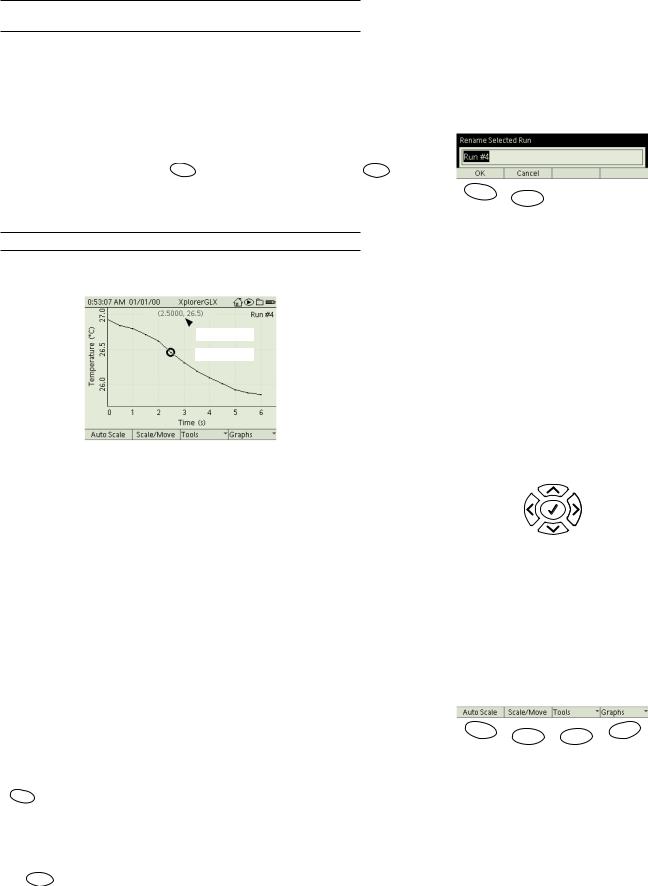
16 G r a p h

In normal mode, one data set is displayed at a time. See “Two Runs” on page 24 for instructions on displaying two runs simultaneously.

The next-to-last option in the run number menu is Delete Run, which deletes the currently displayed run. That run will be deleted from all measurements, not just the one displayed in the Graph.

The last option in the run number menu is Rename Run. By default, data runs are names “Run #1,” “Run #2,” etc. When you select Rename Run, the GLX prompts you for a new run name. Enter the new name using multipress text entry (or an attached keyboard) and press F1 to accept the change (or press F2 to cancel the change). The new name will be applied to that run from all measurements, not just the one displayed in the Graph.

For more information on multipress text entry, see page 90.

Data Cursor and Coordinates

Coordinates

Data Cursor

The circle around one of the data points is the Data Cursor. Use the arrow keys to move the Data Cursor; the left and right arrow keys step the Data Cursor to adjacent data points, the up and down arrow keys make the cursor jump to the first and last visible data points. Press and hold the left and right arrow keys to move the cursor quickly.

The coordinate pair near the top of the Graph indicates the “X” and “Y” values of the Data Cursor.

If you have a mouse, you can move the Data Cursor by dragging it: click on the Data Cursor, hold down the mouse button, and move the mouse left and right to move the Data Cursor along the data plot.

Graph Function Keys

In the Graph, the function keys are used to change the scale and to open the Tools and Graphs menus.

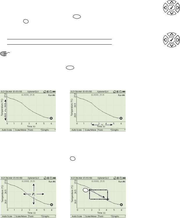
F1 Autoscale

Press F1 to make the scale of the Graph adjust automatically so that all data are visible.

F2 Scale/Move

Pressing F2 cycles the graph through Scale mode (first press) and Move mode (second press).

F1 F2

The GLX prompts you to enter a new data run name

	Jump to
	first point
Step left to	Step right to
adjacent point	adjacent point

Jump to last point

Use the arrow keys to move the Data Cursor

F1	F2	F3	F4

X p l o r e r G L X U s e r s ’ G u i d e

17

In Scale mode, the left and right arrow keys compress and stretch the Graph horizontally; the up and down arrow keys stretch and compress the Graph vertically.

In Move mode, the arrow keys make the graph move left, right, up, and down.

To return to normal mode (indicated when the F2 function reads “Scale/ Move”), press Esc . If the Graph is in Scale or Move mode and the arrow keys are not pressed for several seconds, the Graph will return to normal mode automatically.

See “Zoom” on page 21 for another way to rescale the Graph.

Scale and Move with a Mouse

If you have a mouse, you can scale and move the Graph by dragging it with the mouse cursor. (It is not necessary to press F2 first.)

To change the scale, click and drag on (or between) the numeric labels on the edges of the Graph to change the vertical and horizontal ranges.

Scale	Stretch
Mode	vertically
Compress	Stretch
horizontally	horizontally
	Compress
	vertically
Move	Move up
Mode
Move	Move
left	right

Move down

Arrow key functions in Move and Scale modes

Vertical Scale

Horizontal Scale

To move the plot up, down, left, and right, click and drag anywhere in the “background” of the Graph.

To zoom in on part of the Graph, hold down Esc while you click and drag to draw a rectangle. The area enclosed by the rectangle will enlarge to fill the screen.

Esc

Move

Zoom

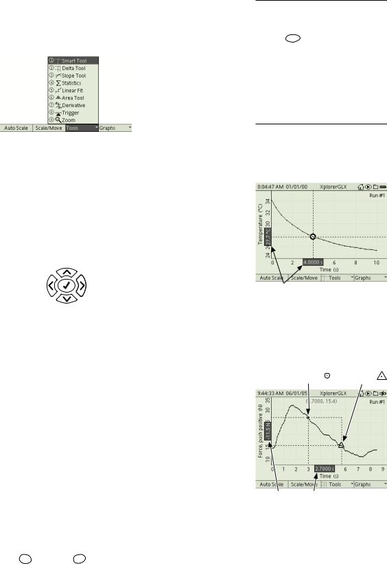
F3 Tools Menu

Use the analysis tools contained in the Tools menu to obtain numerical information from the Graph (such as coordinates and statistics), to visualize different properties of the plotted data (such as slope and area), and to enlarge a selected area. This menu also contains an options to configure the Trigger (see page 20).

18 G r a p h

When you select a tool from the Tools menu,3 a check mark () appears next to it. To turn off a tool, select it from the menu again, which removes the check mark and returns the Graph to normal mode. If you have a tool turned on and you choose a different tool, the previous tool will automatically turn off.

The Tools menu

The options in the Tools menu are described below.

Smart Tool When the Smart Tool is selected from the Tools menu, a pair of crosshairs appears on the Graph with labels indicating its coordinates. Use the left and right arrow keys to move the Smart Tool to adjacent data points. Use the up and down arrow keys to send it to the first and last visible data points. Press and hold the left or right arrow key to move the Smart Tool quickly.

	Jump to
	first point
Step left to	Step right to
adjacent point	adjacent point

Jump to last point

If you have a mouse, you can move the Smart Tool by dragging the circle at the intersection of the cross hairs left and right.

Delta Tool When the Delta Tool is selected from the Tools menu, a dashed rectangle appears on the Graph. One corner is marked with a circle, the other is marked with a triangle. Labels on the edges of the Graph indicate the width (∆X) and height (∆Y) of the rectangle, measured from the circle to the triangle.

When you first turn on the Delta Tool, the circle and triangle appear at the same point. Press the left or right arrow a few times to separate them.

The left and right arrow keys move the triangle to adjacent data points; the up and down arrow keys send the triangle to the first and last visible data points. Press and hold the left or right arrow key to move the triangle quickly.

If you have a mouse, you can move the triangle by dragging it left or right.

The triangle designates the active corner of the Delta Tool, which is the corner that moves when you press the arrow keys or drag it with the mouse. To make the other corner active, hold Esc and press Õ . The triangle and circle will swap places when you release both keys.

Note that when the cursors swap places, the signs of ∆X and ∆Y change. These values are always measured from the circle to the triangle; ∆X is the triangle’s X coordinate minus the circle’s X coordinate, ∆Y is the triangle’s Y coordinate minus the circle’s Y coordinate. You would most typically be interested in the values reported when the triangle is to the right of the circle.

3To select a tool from the Tools menu:

Keypad

1. Press F3 to open the Tools menu.

2.Use the arrow keys to move the highlight to the desired tool and press ; or press the number on the keypad corresponding to the desired tool.

Mouse

1.Click “Tools” at the bottom of the screen to open the Tools menu.

2.Click the desired tool.

Coordinates

Smart Tool

Stationary	Active
Corner	Corner

DY DX

Delta Tool

X p l o r e r G L X U s e r s ’ G u i d e

19

Positive DX and DY

Negative DX and DY

When the cursors swap places, the signs of ∆X and ∆Y change

Slope Tool Select the Slope Tool from the Tools menu to measure the slope of a tangent line at one point on the data plot. A pair of crosshairs marks the point at which the slope is measured. Labels on the Graph’s edges show the coordinates of the point, and the slope is displayed at the bottom of the screen.

Use the left and right arrow keys to move the Slope Tool to adjacent points. Use the up and down arrow keys to send it to the first and last points. Press and hold the left or right arrow key to move the Slope Tool quickly.

If you have a mouse, you can move the Slope Tool by dragging the circle at the intersection of the cross hairs left and right.

Statistics Select Statistics from the Tools menu to put the Graph into Statistics mode. The Graph displays the minimum, maximum, average, and standard deviation (σ) of the data inside the region of interest (ROI), which is indicated by a dashed box.

Region of interest

Active

Cursor

Stationary

Cursor

Slope

Tool

				Slope
Y X
		Slope Tool

Statistics

Statistics mode

Two cursors designate the left and right sides of the ROI. The larger cursor is the active one and can be moved with the arrow keys or mouse.4 As the active cursor moves, one side of the box moves with it.

The smaller cursor indicates the side of the ROI that does not move.

To switch the active cursor to the other side of the box, hold Esc and press Õ .

Linear Fit When Linear Fit is selected from the Tools menu, a best-fit line is applied to the data in the ROI. (See “Statistics” above for instructions on setting the ROI.)

The slope, the Y-intercept, the mean squared error (MSE), and the root mean squared error ( MSE) of the linear fit are displayed at the bottom of the screen along with the correlation coefficient (r) of the data in the ROI.

4See page 16 for detailed instructions on moving the cursor with the keypad or mouse.

Region of interest

Linear Fit

20 G r a p h

When the Linear Fit is turned on, the special option Create Calculation from Linear Fit appears in the Tools menu (see page 22).

Linear Fit can be useful even when the graphed data are not linear (quadratic or exponential, for instance). See “Graph Linearization” on page 47.

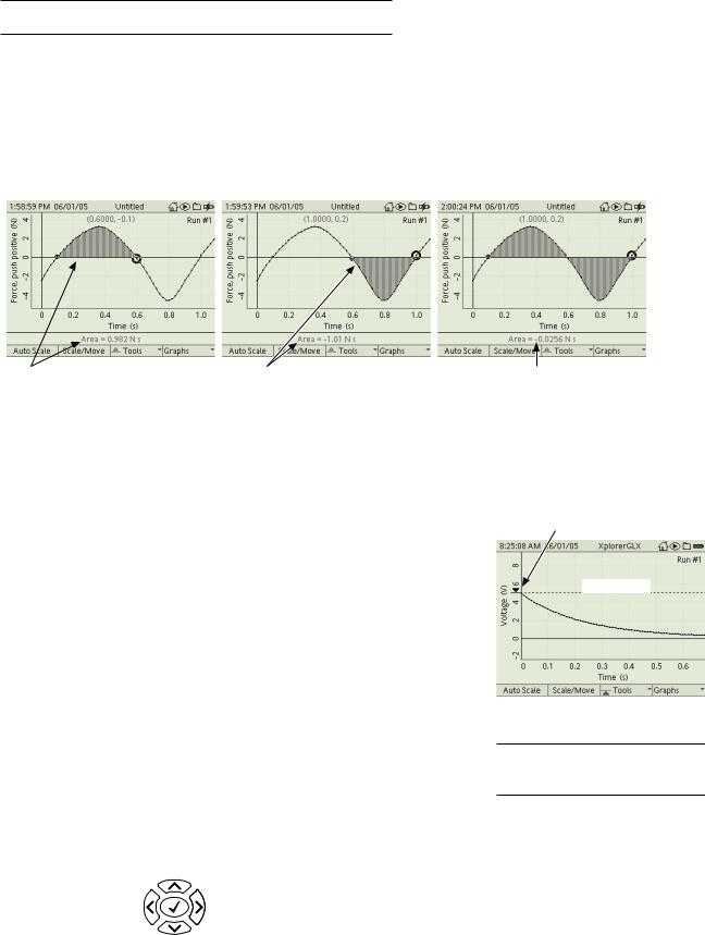
Area Tool Select the Area Tool from the Tools menu to measure the area between the data plot and the X-axis in the ROI. (See “Statistics” above for instructions on setting the ROI.)

For data plotted below the X-axis, the area is measured as negative. The value of area displayed at the bottom of the screen is the total area above the X-axis minus the total area below the X-axis.

Positive	Negative	Total Area is area above the axis minus
Area	Area	area below the axis.
	Area Tool

Derivative This tool overlays a graphical representation of the derivative (or rate of change) of the data. In some cases, the Graph may need to be rescaled in order to see the overlaid derivative. The Derivative Tool is designed for titration experiments in which it is necessary to identify a point in a data set at which the maximum rate of change occurs.

Trigger The Trigger is a tool that allows you to control how the GLX collects data. With the Trigger, you make the GLX delay data recording (after you press ) until a certain condition is met by the incoming data. The Trigger has two parameters: Trigger Edge, which can be rising or falling, and Trigger Level, which specifies the data value that must be crossed. For example, on a voltage versus time graph, if you set the Trigger Edge to rising and the Trigger Level to 5 volts, data recording will not start until the measured voltage rises above 5 volts.

The Trigger can be used in normal graph mode to start continuous recording, or it can be used in Scope Mode (see page 22) to repeatedly trigger bursts of data collection. In both modes, the Graph must have time on the horizontal axis.

To turn on the Trigger, select it from the Tools menu.5 A horizontal dashed line appears on the Graph indicating the Trigger Level. Press the up and down arrow keys to change the Trigger Level. Press the right arrow key to cycle through rising edge, falling edge, and disabled. (The Trigger is initially disabled, so you must press the right arrow key at least once to enable it.)

Increase

Trigger Level

Open Trigger	Enable, Disable, and
Settings	Change Trigger Edge

Decrease

Trigger Level

Arrow Indicating

Trigger Edge

Trigger Level

Trigger

5The Trigger turns on automatically when you turn on Scope mode. See page 22.

X p l o r e r G L X U s e r s ’ G u i d e

21

The Trigger affects data recording even if you are not viewing the Graph. If you have set up two or more triggers on separate Graph pages,6 data recording will start when the most recently set trigger condition is met.

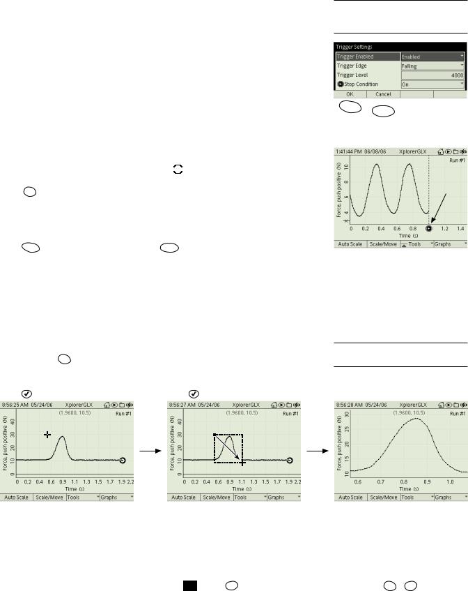
Trigger Settings When the Trigger is turned on, you can open the Trigger Settings dialog box by pressing the left arrow key (you can also select it from the Tools menu). In the dialog box, use the arrow keys to highlight Trigger Enabled and press to enable or disable the Trigger. To change the edge from rising to falling, or vice-versa, use the arrow keys to highlight Trigger Edge and press . To set the level, use the arrow keys to highlight Trigger Level, press , enter the desired value on the keypad, and press again.

You can also turn on the Stop Condition, which causes data collection to automatically stop at a specified time. To turn on the Stop Condition in the Trigger Settings dialog box, use the arrow keys to highlight Stop Condition and press . When the Stop Condition is on, an icon ( ) and vertical dashed line appear on the Graph indicating the stop time. While viewing the Graph, hold down Esc and press the left and right arrow keys to adjust the stop time. For the Stop Condition to work, the Trigger must be turned on (but does need to be enabled).

When you have finished changing the settings in the Trigger Settings dialog box, press F1 to accept the changes, or press F2 to cancel them.

Zoom Use the Zoom Tool to enlarge an area that you define by drawing a rectangle. Select Zoom from the Tools menu; a zoom cursor ( ) appears. Move the cursor (using the arrow keys) to where you want one corner of the rectangle.

Press . Move the cursor to define the diagonally opposite corner of the rectangle. Press again. The area enclosed by the rectangle enlarges to fill the screen.

If you have a mouse, you do not have to open the Tools menu to zoom. Just hold down Esc while you click and drag on the Graph to draw the rectangle.7

Position the cursor to define one corner.		Move the cursor to define the opposite corner.
Press	.	Press	.

Zoom Tool

Swap Cursors This option appears in the Tools menu when you are using the Delta Tool, Statistics, Linear Fit, or Area Tool. When you select Swap Cursors, the active and inactive cursors swap places, allowing you to move the previously stationary corner of the Delta Tool or side of the ROI.

To swap cursors without opening the menu: hold Esc , press Õ , and release both keys.

Toggle Active Data This option appears in the Tools menu when the Graph is in one of the two-data set modes (see pages 23–24). Select it to switch focus from one data set to the other. The active data set is the one to which the Data Cursor

6For information about multiple Graph pages, see “New Graph Page” on page 24.

F1 F2

Trigger Settings dialog box

Stop time

Stop condition

7See also page 17 for other ways to scale the Graph with a mouse.

Area enlarges.

Esc + Õ

Swap Cursors Shortcut

to open the Graphs

22 G r a p h

and other tools are applied. In cases where the two data sets are scaled separately, the active that is scaled.

To toggle data without opening the menu: hold Esc , press , and release both keys.

Create Calculation from Linear Fit This option appears in the Tools menu when the Linear Fit (see page 19) is turned on. Select this option to automatically create an equation in the calculator based on the slope and y-intercept of the currently display best-fit line. If the equation of the best fit line is y = mx + b , where m is the slope and b is the y-intercept, then the calculation will take the form x = (1 ⁄ m)y – b ⁄ m . This calculation will appear in the Calculator and in data source menus with the name “Linear Fit Cal.” For instructions on working with calculations, see page 41.

F4 Graphs Menu

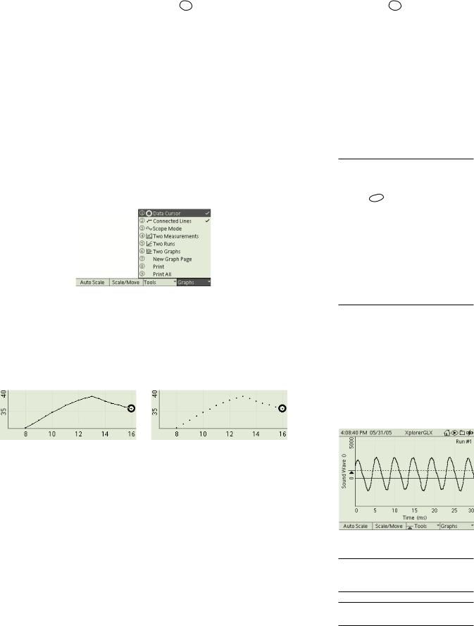
The Graphs menu contains options8 to control the appearance of the Graph, make it emulate an oscilloscope, make it plot two data sets simultaneously, manage multiple pages, and print.

The Graphs menu

Data Cursor Select this option to turn on or off the Data Cursor and Coordinates displayed on the Graph. See page 16 for more information.

Connected Lines Select this option from the Graphs menu to turn on or off the lines connecting the data points.

Graph with connected lines (left) and without connected lines (right)

Scope Mode Select Scope mode from the Graphs menu to make the GLX emulate a digital storage oscilloscope. In this mode, the GLX collects and displays data in repeated bursts. The length of the burst and the sample rate are determined by the time scale of the Graph display. Scope mode can be used with any sensor to collect bursts of data; it is especially useful with the GLX’s built-in sound sensor (see page 58) or voltage sensor.

When you turn on Scope mode, the Graph automatically sets its time range to 30 milliseconds and turns on the Trigger.9 It also adjusts the sampling rate of the displayed sensor so that it will collect about 500 data points (or as many as possible) in each burst. If you change the Graph’s time scale,10 the GLX automatically adjusts the sampling rate.

Esc +

Toggle Data Shortcut

8To select an option from the Graphs menu

Keypad

1. Press F4

menu.

2.Use the arrow keys to move the high-

light to the desired menu option and press ; or press the number on the keypad corresponding to the desired

menu option.

Mouse

1.Click “Graphs” at the bottom of the screen to open the Graphs menu.

2.Click the desired menu option.

Scope mode

9The Trigger is initially disabled. See page 20 for instructions on enabling and setting the Trigger.

10See “F1 Autoscale” and “F2 Scale/ Move” on page 16.

X p l o r e r G L X U s e r s ’ G u i d e

23

After you press , the GLX begins collecting and displaying a series of data bursts (each burst is enough data fill the Graph from left to right). If you have enabled the Trigger, the GLX waits for the trigger condition to be met before collecting each burst.

While Scope-mode data collection is in progress, you can change the scale of the Graph (with F1 Autoscale, F2 Scale/Move, or the mouse) and you can change the Trigger settings with the arrow keys.

To stop data collection, press again. The GLX will save the last-collected data burst as Run #1 (or #2, #3, #4, etc.). You can also use the Trigger’s Stop Condition (see page 21) to make the GLX stop automatically after collecting a single data burst.

You can use Scope Mode in conjunction with Two Measurements mode or

Two Graphs mode (see below) to display two traces simultaneously.

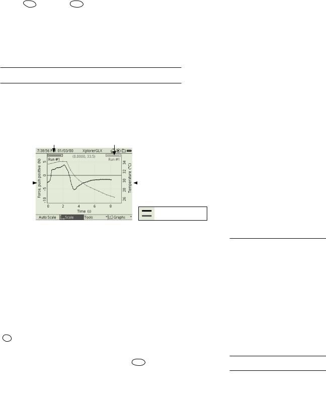
Two Measurements Select this option from the Graphs menu to put the Graph into Two Measurements mode. In this mode, two measurements (or data sets) are graphed simultaneously.

Run Number of	Run Number of
First Measurement	Second Measurement
(select to change)	(select to change)

Data Source of				Data Source of
First Measurement				Second Measurement
(select to change)				(select to change)

Active Data (black)

Inactive Data (gray)

Two Measurements mode

The data source and scale of the First Measurement are displayed on the left side, and the data source and scale of the Second Measurement is displayed on the right side. Select either the left or right data source field11 to change the corresponding measurement.

The run number of the First Measurement is displayed in the upper left corner of the Graph, and the run number of the Second Measurement is displayed in the upper right corner. To change the run number of either measurement, select the corresponding run number field.11

One of the measurements is plotted in black, and the other one in gray. The measurement in black is the active data. To switch activity to the other measurement, hold Esc and press .

The Data Cursor appears on the active data. If you select a tool from the Tools menu, it is applied to the active data set. If you press F2 to scale or move vertically, only the active data will change.12 However, moving the Graph horizontally or changing the horizontal scale will affect both sets.

If you are using a mouse, you can switch activity to a measurement by clicking on the line above its run number. Vertically scale each measurement by dragging its numeric labels (on the left or right side of the Graph).

11To select a data source field or run number field:

Keypad

1.Press to light up the active fields.

2.Use the arrow keys to move the highlight to the desired field.

3.Press again to open the menu.

4.Use the arrow keys to move the high-

light to the desired menu option and press ; or press the number on the keypad corresponding to the desired

menu option.

Mouse

1.Click the desired field to open the menu.

2.Click the desired menu option.

12The exception to this rule is when both data sets are of the same units (both temperature in °C, for instance); in that case, both data sets scale together.

24G r a p h

Typically you would use Two Measurements mode to display data from two different sources, but you can also use it to display two runs from the same source. Select the same source from both data source fields, and different runs from each run number field. For another way to display two runs from the same source, see “Two Runs” below.

Two Runs Select Two Runs from the Graphs menu to display two data sets from a single data source.

In this mode, a second run appears on the Graph. A second run number field appears in the upper right corner (below the first run number), which you can select to choose a different run.

One of the runs is plotted in black, and the other one in gray. The run in black is the active data. To switch activity to the other run, hold Esc and press . The Data Cursor appears on the active data. If you select a tool from the Tools menu, it is applied to the active data set.

Both runs share a single pair of axes and they are scaled and moved together.

If you are using a mouse, you can switch activity to a run by clicking on the line above its run number.

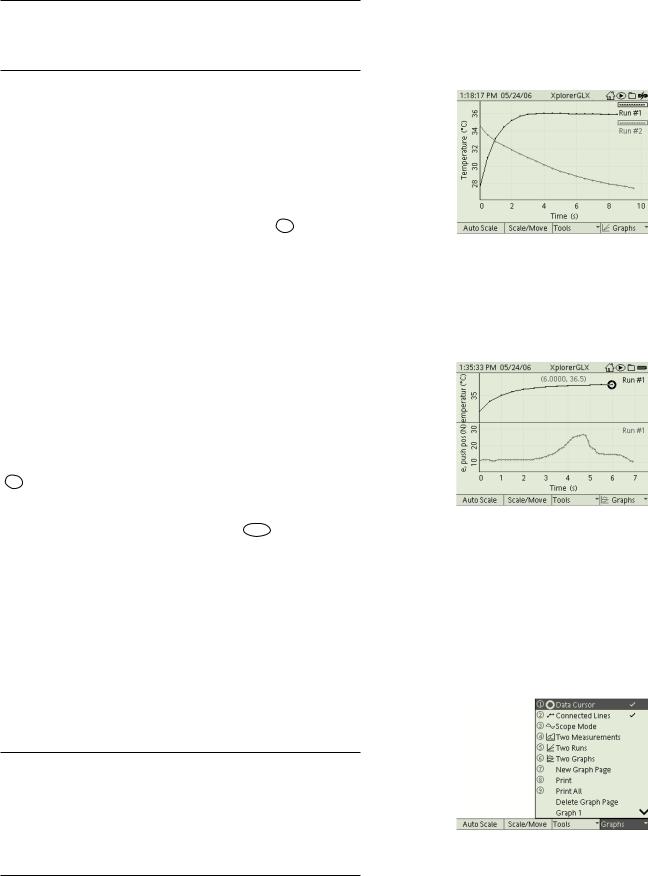
Two Graphs Select Two Graphs from the Graphs menu to display two separate graphs simultaneously. This mode is similar to Two Measurements mode (see page 23), but each measurement is plotted on the top or bottom half of the screen, rather than overlapping.

One of the measurements is plotted in black, and the other one in gray. The measurement in black is the active data. To switch activity to the other measurement, hold Esc and press .

The Data Cursor appears on the active data. If you select a tool from the Tools menu, it is applied to the active data. If you press F2 to scale or move vertically, only the active data will change. However, moving the Graph horizontally or changing the horizontal scale will affect both sets.

If you are using a mouse, you can switch activity to a measurement by clicking on it.

New Graph Page The GLX supports an unlimited number of graph pages. Select New Graph Page from the Graphs menu to configure a new graph while preserving the previous one.

When two or more graph pages exist, each page appears in the Graphs menu. To make a page visible, select it from the menu.

If added graph pages make the Graphs menu too long to fit on the screen, an arrow or arrows ( , ) will appear on the right side of the menu to indicate that some of the menu options are not visible.

Press the up or down arrow key multiple times to move the highlight beyond the visible portion of the menu. The menu will scroll to bring other options into view.

If you are using a mouse, you can click the arrows to scroll the menu.

Two Runs mode

Two Graphs mode

The Graphs menu as it appears when multiple pages exist