Sharp EL-5230, EL-5250 User Manual

®

EL-5230

EL-5250

PROGRAMMABLE SCIENTIFIC CALCULATOR

OPERATION MANUAL

SHARP EL-5230/5250

Programmable Scientific Calculator

Introduction

Chapter 1:

Before You Get Started

Chapter 2:

General Information

Chapter 3:

Scientific Calculations

Chapter 4:

Statistical Calculations

Chapter 5:

Equation Solvers

Chapter 6:

Complex Number Calculations

Chapter 7:

Programming

Chapter 8:

Application Examples

Appendix

1

Contents
Introduction ...........................................................	7
Operational Notes ....................................................................................	8
Key Notation in This Manual ....................................................................	9
Chapter 1: Before You Get Started .....................	11
Preparing to Use the Calculator ............................................................	11
Resetting the calculator .................................................................	11
The Hard Case .......................................................................................	12
Calculator Layout and Display Symbols ................................................	13
Operating Modes ...................................................................................	15
Selecting a mode ...........................................................................	15
What you can do in each mode .....................................................	15
A Quick Tour ...........................................................................................	16
Turning the calculator on and off ...................................................	16
Entering and solving an expression ...............................................	16
Editing an expression .....................................................................	17
Using variables ...............................................................................	18
Using simulation calculations (ALGB) ...........................................	19
Using the solver function ................................................................	21
Other features ................................................................................	22
Chapter 2: General Information .........................	23
Clearing the Entry and Memories ..........................................................	23
Memory clear key ...........................................................................	23
Editing and Correcting an Equation ......................................................	24
Cursor keys ....................................................................................	24
Overwrite mode and insert mode ..................................................	24
Delete key .......................................................................................	25
Multi-entry recall function ...............................................................	25
The SET UP menu .................................................................................	26
Determination of the angular unit ..................................................	26
Selecting the display notation and number of decimal places ......	26

2

Contents
Setting the floating point numbers system in scientific notation	... 26
Using Memories .....................................................................................	27
Using alphabetic characters ..........................................................	27
Using global variables ....................................................................	27
Using local variables ......................................................................	28
Using variables in an equation or a program .................................	29
Using the last answer memory ......................................................	30
Global variable M ...........................................................................	30
Using memory in each mode .........................................................	31
Resetting the calculator .................................................................	32
Chapter 3: Scientific Calculations .....................	33
NORMAL mode ......................................................................................	33
Arithmetic operations .....................................................................	33
Constant calculations .....................................................................	34
Functions ................................................................................................	34
Math menu Functions ............................................................................	36
Differential/Integral Functions ................................................................	38
Differential function ........................................................................	38
Integral function ..............................................................................	39
When performing integral calculations ..........................................	40
Random Function ..................................................................................	41
Random numbers ...........................................................................	41
Random dice ..................................................................................	41
Random coin ..................................................................................	41
Random integer ..............................................................................	41
Angular Unit Conversions ......................................................................	42
Chain Calculations .................................................................................	42
Fraction Calculations .............................................................................	43
Binary, Pental, Octal, Decimal and Hexadecimal Operations (N-base) ...	44
Time, Decimal and Sexagesimal Calculations ......................................	46
Coordinate Conversions ........................................................................	47
Calculations Using Physical Constants .................................................	48
Calculations Using Engineering Prefixes ..............................................	50
Modify Function ......................................................................................	51

3

Contents
Solver Function ......................................................................................	52
Entering and solving an equation ..................................................	52
Changing the value of variables and editing an equation .............	52
Solving an equation .......................................................................	53
Important notes ..............................................................................	54
Simulation Calculation (ALGB) ..............................................................	55
Entering an expression for simulation calculation .........................	55
Changing a value of variables and editing an expression .............	55
Simulate an equation for different values ......................................	56
Filing Equations .....................................................................................	58
Saving an equation ........................................................................	58
Loading and deleting an equation .................................................	59
Chapter 4: Statistical Calculations ....................	61
Single-variable statistical calculation .............................................	62
Linear regression calculation .........................................................	62
Exponential regression, logarithmic regression,
power regression, and inverse regression calculation ..................	62
Quadratic regression calculation ...................................................	63
Data Entry and Correction .....................................................................	63
Data entry .......................................................................................	63
Data correction ...............................................................................	63
Statistical Calculation Formulas ............................................................	65
Normal Probability Calculations ............................................................	66
Statistical Calculations Examples .........................................................	67
Chapter 5: Equation Solvers ..............................	69
Simultaneous Linear Equations .............................................................	69
Quadratic and Cubic Equation Solvers .................................................	71
Chapter 6: Complex Number Calculations .......	73
Complex Number Entry .........................................................................	73
Chapter 7: Programming ....................................	75
PROG mode ...........................................................................................	75

4

	Contents
Entering the PROG mode ..............................................................	75
Selecting the NORMAL program mode or the NBASE
program mode ................................................................................	75
Programming concept ....................................................................	75
Keys and display ............................................................................	76
Creating a NEW Program ......................................................................	76
Creating a NEW program ...............................................................	76
Use of variables ..............................................................................	77
Programming Commands ......................................................................	79
Input and display commands .........................................................	79
Flow control ....................................................................................	81
Equalities and inequalities .............................................................	82
Statistical Commands ............................................................................	83
Editing a Program ..................................................................................	84
Error Messages ......................................................................................	85
Deleting Programs .................................................................................	86
Chapter 8: Application Examples ......................	87
Programming Examples ........................................................................	87
Some like it hot (Celsius-Fahrenheit conversion) ..........................	87
The Heron Formula ........................................................................	89
2B or not 2B (N-base conversion) .................................................	91
T test ...............................................................................................	93
A circle that passes through 3 points ............................................	95
Radioactive decay ..........................................................................	97
Delta-Y impedance circuit transformation .....................................	99
Obtaining tensions of strings .......................................................	102
Purchasing with payment in n-month installments ......................	104
Digital dice ....................................................................................	106
How many digits can you remember? .........................................	107
Calculation Examples ..........................................................................	110
Geosynchronous orbits ................................................................	110
Twinkle, twinkle, little star (Apparent magnitude of stars) ...........	111
Memory calculations ....................................................................	113
The state lottery ...........................................................................	114

5

Contents
Appendix ............................................................	115
Battery Replacement ...........................................................................	115
Batteries used ..............................................................................	115
Notes on battery replacement .....................................................	115
When to replace the batteries ......................................................	115
Cautions .......................................................................................	116
Replacement procedure ...............................................................	116
Automatic power off function ........................................................	117
The OPTION menu ..............................................................................	118
The OPTION display ....................................................................	118
Contrast ........................................................................................	118
Memory check ..............................................................................	118
Deleting equation files and programs ..........................................	119
If an Abnormal Condition Occurs ........................................................	119
Error Messages ....................................................................................	120
Using the Solver Function Effectively ..................................................	121
Newton’s method ..........................................................................	121
‘Dead end’ approximations ...........................................................	121
Range of expected values ............................................................	121
Calculation accuracy ....................................................................	122
Changing the range of expected values ......................................	122
Equations that are difficult to solve ..............................................	123
Technical Data .....................................................................................	124
Calculation ranges .......................................................................	124
Memory usage .............................................................................	126
Priority levels in calculations ........................................................	127
Specifications .......................................................................................	128
For More Information about Scientific Calculators ..............................	129

6

Introduction

Thank you for purchasing the SHARP Programmable Scientific Calculator

Model EL-5230/5250.

After reading this manual, store it in a convenient location for future reference.

•Unless the model is specified, all text and other material appearing in this manual applies to both models (EL-5230 and EL-5250).

•Either of the models described in this manual may not be available in some countries.

•Screen examples shown in this manual may not look exactly the same as what is seen on the product. For instance, screen examples will show only the symbols necessary for explanation of each particular calculation.

•All company and/or product names are trademarks and/or registered trademarks of their respective holders.

7

Introduction

Operational Notes

•Do not carry the calculator around in your back pocket, as it may break when you sit down. The display is made of glass and is particularly fragile.

•Keep the calculator away from extreme heat such as on a car dashboard or near a heater, and avoid exposing it to excessively humid or dusty environments.

•Since this product is not waterproof, do not use it or store it where fluids, for example water, can splash onto it. Raindrops, water spray, juice, coffee, steam, perspiration, etc. will also cause malfunction.

•Clean with a soft, dry cloth. Do not use solvents or a wet cloth.

•Do not drop it or apply excessive force.

•Never dispose of batteries in a fire.

•Keep batteries out of the reach of children.

•This product, including accessories, may change due to upgrading without prior notice.

NOTICE

•SHARP strongly recommends that separate permanent written records be kept of all important data. Data may be lost or altered in virtually any electronic memory product under certain circumstances. Therefore, SHARP assumes no responsibility for data lost or otherwise rendered unusable whether as a result of improper use, repairs, defects, battery replacement, use after the specified battery life has expired, or any other cause.

•SHARP will not be liable nor responsible for any incidental or consequential economic or property damage caused by misuse and/ or malfunctions of this product and its peripherals, unless such liability is acknowledged by law.

8

Introduction

Key Notation in This Manual

In this manual, key operations are described as follows:

	To specify ex : @".....................
	To specify In : i
	To specify F	: ;F ...........................
	To specify d/c : @F.....................
	To specify ab/c: k
	To specify H	: ;H ...........................
	To specify i	: Q..............................

Functions that are printed in orange above the key require @to be pressed first before the key.

When you specify the memory (printed in blue above the key), press ;first.

Alpha-numeric characters for input are not shown as keys but as regular alpha-numeric characters.

Functions that are printed in grey (gray) adjacent to the keys are effective in specific modes.

Note:

•To make the cursor easier to see in diagrams throughout the manual, it is depicted as ‘_’ under the character though it may actually appear as a rectangular cursor on the display.

Example

Press j @s;R

A k S 10

•@s and ;R means you have to press @followed by `key and

;followed by 5key.

NORMAL MODE 0.

πRŒ˚–10_

9

10

Chapter 1

Before You Get Started

Preparing to Use the Calculator

Before using your calculator for the first time, you must reset it and adjust its contrast.

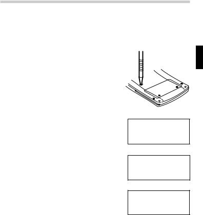
Resetting the calculator

1.Press the RESET switch located on the back of the calculator with the tip of a ballpoint pen or similar object. Do not use an object with a breakable or sharp tip.

•If you do not see the message on the right, the battery may be installed incorrectly; refer to ‘Battery Replacement’

(See page 115.) and try installing it again.

2.Press y.

•The initial display of the NORMAL mode appears.

3.Press @o0and press +or

-to adjust the display contrast until it is set correctly, then press j.

•@omeans you have to press @ followed by S key.

zALL DATA CL?z z YES¬[DEL] z z NO¬[ENTER]z

NORMAL MODE 0.

LCD CONTRAST [+] [-] DARK® ¬LIGHT

•See ‘The OPTION menu’ (See page 118.) for more information regarding optional functions.

11

Chapter 1: Before You Get Started

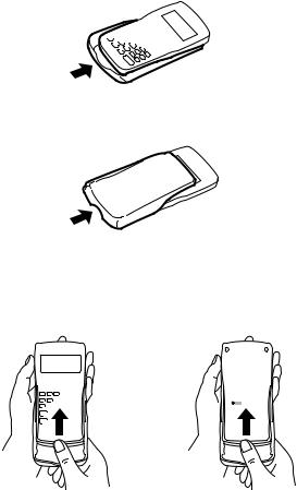
The Hard Case

Your calculator comes with a hard case to protect the keyboard and display when the calculator is not in use.

Before using the calculator, remove the hard case and slide it onto the back as shown to avoid losing it.

When you are not using the calculator, slide the hard case over the keyboard and display as shown.

•Firmly slide the hard case all the way to the edge.

•The quick reference card is located inside the hard case.

•Remove the hard case while holding with fingers placed in the positions shown below.

12

Chapter 1: Before You Get Started

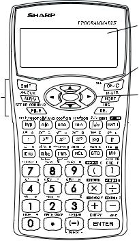
Calculator Layout and Display Symbols

Calculator layout

1 Display screen

2 Power ON/OFF

and Clear key

	3 Key operation	4 Cursor keys
	keys

1Display screen: The calculator display consists of 14 × 3 line dot matrix display (5 × 7 dots per character) and a 2-digit exponent display per each line.

2Power ON/OFF and Clear key: Turns calculator ON. To turn off the calculator, press @, then o. This key can also be used to clear the display.

3Key operation keys:

@: Activates the second function (printed in orange) assigned to the next pressed key.

;: Activates the variable (printed in blue) assigned to the next pressed key.

4 Cursor keys: Enables you to move the cursor in four directions.

13

Chapter 1: Before You Get Started

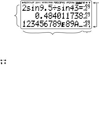
Display

Symbol

Dot matrix display

Exponent

Mantissa

•During actual use, not all symbols are displayed at the same time.

•Only the symbols required for the usage under instruction are shown in the display and calculation examples of this manual.

		:	Indicates some contents are hidden in the directions shown.
			Press cursor keys to see the remaining (hidden) section.
BUSY		:	Appears during the execution of a calculation.
2ndF		:	Appears when @is pressed.
xy/rθ		:	Indicates the mode of expression of results in the complex
			calculation mode.
HYP		: Indicates that H has been pressed and the hyperbolic functions
			are enabled. If @>are pressed, the symbols ‘2ndF HYP’
			appear, indicating that inverse hyperbolic functions are enabled.
ALPHA: Appears when ;, @a, x or tis pressed.
FIX/SCI/ENG: Indicates the notation used to display a value.
DEG/RAD/GRAD: Indicates angular units.
		: Appears when statistics mode is selected.
M		: Indicates that a value is stored in the M memory.

14

Chapter 1: Before You Get Started

Operating Modes

This calculator has five operating modes to perform various operations. These modes are selected from the MODE key.

Selecting a mode

1.Press b.

The menu display appears.

Press dto display the next menu page.

<MODE-1> ƒNORMAL ⁄STAT ¤PROG ‹EQN

<MODE-2> ›CPLX

2.Press 0to select the NORMAL mode.

•In the menu display, press the assigned number to choose or recall a selection.

What you can do in each mode

NORMAL mode:

NORMAL MODE 0.

Allow you to perform standard scientific calculations, Differential/Integral functions, N-base calculations, Solver function, Simulation calculation.

STAT (statistics) mode:

Allows you to perform statistical calculations.

PROG (program) mode:

Allows you to create and use programs to automate simple or complex calculations.

EQN (equation) mode:

Allows you to perform equation solvers, such as quadratic equation.

CPLX (complex) mode:

Allows you to perform arithmetic operations with complex numbers.

15

Chapter 1: Before You Get Started

A Quick Tour

This section takes you on a quick tour covering the calculator’s simple arithmetic operations and also principal features like the solver function.

Turning the calculator on and off

1.Press j at the top right of the keypad to turn the calculator on.

•To conserve the batteries, the calculator turns itself off automatically if it is not used for several minutes.

NORMAL MODE 0.

2.Press @o to turn the calculator off.

•Whenever you need to execute a function or command which is written in orange above a key, press @followed by the key.

Entering and solving an expression

Arithmetic expressions should be entered in the same order as they would normally be written in. To calculate the result of an expression, press eat the bottom right of the keypad; this has the same function as the ‘equals’ key on some calculators.

Example

Find the answer to the expression

82 ÷ 3 – 7 × -10.5

1.8 Az @*3 -

7 kS 10.5

•This calculator has a minus key - for subtraction and a negative key S for entering negative numbers.

NORMAL MODE 0.

8Œ©‰3-7˚–10.5_

•To correct an error, use the cursor keys

lrudto move to the appropriate position on the display and type over the original expression.

2.Press eto obtain an answer.

•While the calculator is computing an answer, BUSY is displayed at the above left of the display.

•The cursor does not have to be at the end of an expression for you to obtain an answer.

0. 8Œ©‰3-7˚–10.5= 110.4504172

16

Chapter 1: Before You Get Started

Editing an expression

After obtaining an answer, you can go back to an expression and modify it using the cursor keys just as you can before the eis pressed.

Example

Return to the last expression and change it to 82 ÷ 3 – 7 × -10.5

	1. Press dor rto return to the
		8Œ©‰3-7˚–10.5=
	last expression.
	• The cursor is now at the beginning of	110.4504172
		8Œ©‰3-7˚–10.5
	the expression (on ‘8’ in this case).

•Pressing uor lafter obtaining an answer returns the cursor to the end of the last expression.

•To make the cursor easier to see in diagrams throughout the manual, it is depicted as ‘_’ under the character though it may actually appear as a rectangular cursor on the display.

2.Press rfour times to move the cursor to the point where you wish to make a change.

•The cursor has moved four places to the right and is now flashing over ‘3’.

3.Press @O.

8Œ©‰3-7˚–10.5= 110.4504172 8Œ©‰3-7˚–10.5

•This changes the character entering mode from ‘overwrite’ to ‘insert’.

•When @is pressed the 2ndF symbol should appear at the above of the display. If it does not, you have not pressed the key firmly enough.

•The shape of the flashing cursor tells you which character entering mode you are in. A triangular cursor indicates ‘insert’ mode while a rectangular cursor indicates ‘overwrite’ mode.

4.Press (and then move the cursor to the end of expression (@r).

•Note that the cursor has moved to the second line since the expression now exceeds 14 characters.

5.Press )and eto find the answer for the new expression.

110.4504172 8Œ©‰(3-7˚–10.5

8Œ©‰(3-7˚–10.5 )= 7.317272966

17

Chapter 1: Before You Get Started

Using variables

You can use 27 variables (A-Z and θ) in the NORMAL mode. A number stored as a variable can be recalled either by entering the variable name or using t.

Example 1

Store 23 to variable R.

1.Press j 2 1 then x.

• j clears the display.

• ALPHA appears automatically when you press x. You can now enter any alphabetic character or θ (written in blue above keys in the keypad).

2.Press R to store the result of 23 in R.

•The stored number is displayed on the next line.

•ALPHA disappears from the display.

You can also store a number directly

rather than storing the result of an expression.

NORMAL MODE 0.

2„Ò_

0. 2„ÒR

8.

Example 2

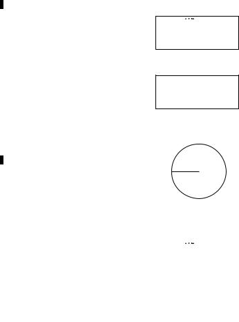
Find the area of a circle which has radius R.

r

S = πr2

	Enter an expression containing variable R (now equal to 8) from the last
	example.
	1. Press j @s then ;.
		NORMAL MODE
	• Whenever you need to use a character
		0.
	written in blue on the keypad, press
		π_
	;beforehand. ALPHA will appear at
	the above of the display.
	2. Press R and then A.
		NORMAL MODE
	• ALPHA disappears after you have
		0.
	entered a character.
		πRŒ_

18

Chapter 1: Before You Get Started

3.Press eto obtain the result.

Follow the same procedure as above, but press t instead of ;in step 1.

You will get the same result.

0.

πRŒ=

201.0619298

Using simulation calculations (ALGB)

If you want to find more than one solution using the same formula or algebraic equation, you can do this quickly and simply by use of the simulation calculation.

Example

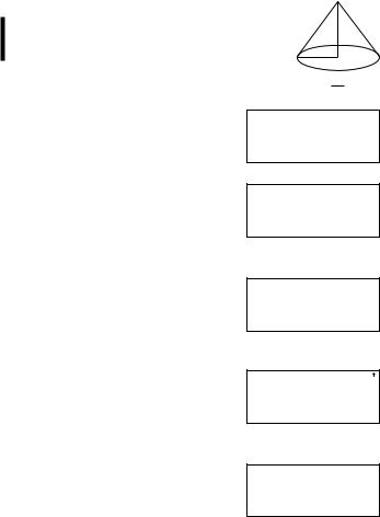
Find the volume of two cones:

1 with height 10 and radius 8 and

2 with height 8 and radius 9.

1.Press j1 k3 @s

;R A;H to enter the formula.

•Note that ‘13’ represents 1 over (i.e. divided by) 3.

•Variables can be represented only by capital letters.

2.Press @G(I key) to finish entering the equation.

•The calculator automatically picks out the variables alphabetically contained in the equation in alphabetical order and asks you to input numbers for them.

h

r

V = 13 πr2h

NORMAL MODE 0.

1ı3πRŒH_

1ı3πRŒH

H=z 0.

• at the bottom of the display reminds you that there is another variable further on in the expression.

3.Press 10 eto input the height and go on the next variable.

•The calculator is now asking you to input a number for the next variable.

1ı3πRŒH

R=z 8.

19

Chapter 1: Before You Get Started

•Note that, as the variable R already has a number stored in memory, the calculator recalls that number.

• indicates that there is another variable earlier in the expression.

4.Press 8 to input the radius.

Input of all variables is now complete.

5.Press eto obtain the solution.

•The answer (volume of cone ) is displayed on the third line.

6.Press eand 8 to input the height for cone .

•The display returns to a value entry screen with ‘8’ substituted for ‘10’ in variable H.

7.Press eto confirm the change.

8.Press 9 to enter the new radius then press eto solve the equation.

•The volume of cone is now displayed.

•In any step, press @hto obtain the solution using the values entered into the variables at that time.

1ı3πRŒH=

670.2064328

1ı3πRŒH H=8_

1ı3πRŒH
R=z	8.

1ı3πRŒH=

678.5840132

20

Chapter 1: Before You Get Started

Using the solver function

You can solve any unknown variable in an equation by assigning known values to the rest of the variables. Let us compare the differences between the solver function and the simulation calculations using the same expression as in the last example.

Example

	What is the height of cone 3 if it has a radius of 8	h
	and the same volume as cone 2 (r = 9, h = 8) in
	the last example?	r

9.Store the result of step 8 on the previous page in variable V. Press jtwice and ;< xV.

10.Input the equation (including ‘=’) in the NORMAL mode.

Press ;V ;=then input the rest of the expression.

You must press ;=( m key), not e, to enter the = sign.

V = 13 πr2h

0.

AnsÒV

678.5840132

AnsÒV 678.5840132 V=1ı3πRŒH_

11.Press I 5to move to the variable input display.

•Note that the values assigned to the variables in the last example for the simulation calculations are retained and displayed.

12.Press dto skip the height, and then press 8 eto enter the radius

(R).

•The cursor is now on V. The value that was stored in step 9 is displayed.

(volume of cone 2)

13.Press uuto go back to the variable H.

•This time the value of H from memory is also displayed.

V=1ı3πRŒH

H=z 8.

V=1ı3πRŒH

V=z678.5840132

V=1ı3πRŒH

H=z 8.

21

Chapter 1: Before You Get Started

14.Press @hto find the height of cone 3.

•Note that the calculator finds the value of the variable that the cursor is on when you press @h.

•Now you have the height of cone 3 that has the same volume as cone

2.

H=	10.125

R¬ 678.5840132 L¬ 678.5840132

Right and left sides of the expression after substituting the known variables

Height of cone 3

•R→ and L→ are the values computed

by Newton's method, which is used to determine the accuracy of the solution.

Other features

Your calculator has a range of features that can be used to perform many calculations other than those we went through in the quick tour. Some of the important features are described below.

Statistical calculations:

You can perform oneand twovariable weighted statistical calculations, regression calculations, and normal probability calculations. Statistical results include mean, sample standard deviation, population standard deviation, sum of data, and sum of squares of data. (See Chapter 4.)

Equation solvers:

You can perform solvers of simultaneous linear equation with two/three unknowns or quadratic/cubic equation. (See Chapter 5.)

Complex number calculations:

You can perform addition, subtraction, multiplication, and division calculations. (See Chapter 6.)

Programming:

You can program your calculator to automate certain calculations. Each program can be used in either the NORMAL or NBASE program modes. (See Chapter 7.)

22

Chapter 2

General Information

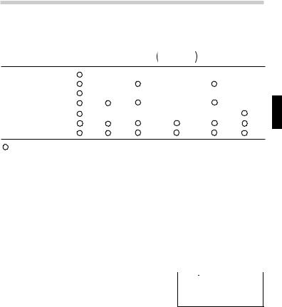
Clearing the Entry and Memories

Operation	Entry	Local	Saved equations*2	Multi-entry	STAT*4
			including saved	recall,
	(Display) A- Z, θ*1	variables	local variables	ANS*3	STAT VAR*5

j		×	×	×	×	×
Mode selection		×	×	×	×	×*6
@ P 0		×		×		×
@ P 1 y		×	×	×	×	×
@ P 2 y				×
@ P 3 y
RESET switch
	: Clear	×: Retain
*1	Global variable memories.
*2	Saved equations and local variables by the filing equations function
*3	Last answer memory.
*4	Statistical data (entered data)
*5 n, ¯x, sx, σx, Σx, Σx2, y¯, sy, σy, Σy, Σy 2, Σxy, a, b, c, r.
*6	Will be cleared when changing between sub-modes in the STAT mode.

Note:

•To clear one variable memory of global variable and local variable memories, press j x and then choose memory.

	Memory clear key
	Press @ P to display the menu.
		<M-CLR>
	• To initialize the display mode, press 0.
		ƒDISP	⁄MEMORY
	The parameters set as follows.	¤STAT	‹RESET

•Angular unit: DEG (See page 26.)

•Display notation: NORM1 (See page 26.)

•N-base: DEC (See page 44.)

•To clear all variables (excluding local variables of saved equations, statistical data and STAT variables), press 1 y.

•To clear statistical data and STAT variables, press 2 y.

•To RESET the calculator, press 3 y. The RESET operation will erase all data stored in memory and restore the calculator’s default setting.

23

Chapter 2: General Information

Editing and Correcting an Equation

Cursor keys

Incorrect keystrokes can be changed by using the cursor keys

(lrud).

Example

Enter 123456 then correct it to 123459.

1.Press j 123456.

NORMAL MODE 0.

123456_

2.Press y9 e.

•If the cursor is located at the right end of an equation, the ykey will function as a backspace key.

0.

123459=

123459.

•You can return to the equation just after

getting an answer by pressing the cursor keys. After returning to the equation, the following operations are useful;

@lor @r: To jump the cursor to the beginning or the end of equation.

Overwrite mode and insert mode

•Pressing @O switches between the two editing modes: overwrite mode (default); and insert mode. A rectangular cursor indicates preexisting data will be overwritten as you make entries, while a triangular cursor indicates that an entry will be inserted at the cursor.

•In the overwrite mode, data under the cursor will be overwritten by the number you enter. To insert a number in the insert mode, move the cursor to the place immediately after where you wish to insert, then make the desired entry.

•The mode set will be retained until @O is pressed or a RESET operation is performed.

24

Chapter 2: General Information

Delete key

•To delete a number/function, move the cursor to the number/function you wish to delete, then press y. If the cursor is located at the right end of an equation, the ykey will function as a backspace key.

Multi-entry recall function

Previous equations can be recalled in the NORMAL, STAT or CPLX mode.

Up to 160 characters of equations can be stored in memory.

When the memory is full, stored equations are deleted in the order of the oldest first.

•Pressing @gwill display the previous equation. Further pressing @gwill display preceding equations.

•You can edit the equation after recalling it.

•The multi-entry memory is cleared by the following operations: mode change, memory clear (@P 1y), RESET, N-base conversion.

Example

Input three expressions and then recall them.

13(5+2)=

23×5+2=

33×5+3×2=

1.Press j 3 (5 +2 )e 3 k 5 +2 e

3 k 5 +3 k 2 e

2.Press @gto recall the expression 3.

17. 3˚5+3˚2= 21.

3˚5+3˚2= 21. 3˚5+3˚2

3.Press @gto recall the expression 2.

4.Press @gto recall the expression 1.

3˚5+3˚2= 21. 3˚5+2

3˚5+3˚2= 21. 3(5+2)

25

Chapter 2: General Information

The SET UP menu

The SET UP menu enables you to change the angular unit and the display format.

•Press @J to display the SET UP menu.

•Press j to exit the SET UP menu.

Determination of the angular unit

The following three angular units (degrees, radians, and grads) can be specified.

• DEG(°) : Press @J 00

•RAD (rad): Press @J 01

•GRAD (g) : Press @J 02

<SET UP>

ƒDRG ⁄FSE ¤---

Selecting the display notation and number of decimal places

Five display notation systems are used to display calculation results: Two settings of Floating point (NORM1 and NORM2), Fixed decimal point (FIX), Scientific notation (SCI) and Engineering notation (ENG).

•When @J 10(FIX) or @J 12(ENG) is pressed, ‘TAB(0-9)?’ will be displayed and the number of decimal places

(TAB) can be set to any value between 0 and 9.

•When @J 11(SCI) is pressed, ‘SIG(0-9)?’ will be displayed and the number of significant digits (SIG) can be set to any value between 0 and 9. Entering 0 will set a 10-digit display.

•When a floating point number does not fit in the specified range, the calculator will display the result using the scientific notation (exponential notation) system. See the next section for details.

Setting the floating point numbers system in scientific notation

The calculator has two settings for displaying a floating point number:

NORM1 (default setting) and NORM2. In each display setting, a number is automatically displayed in scientific notation outside a preset range:

•NORM1: 0.000000001 ≤ |x| ≤ 9999999999

•NORM2: 0.01 ≤ |x| ≤ 9999999999

26

Chapter 2: General Information

Example	Key operations	Result
100000÷3=	j@J13
[Floating point (NORM1)]	100000z 3e	33333.33333
→[FIXed decimal point	@J102	33333.33
and TAB set to 2]		3.33˚1004
→[SCIentific notation	@J113
and SIG set to 3]		33.33˚1003
→[ENGineering notation	@J122
and TAB set to 2]
→[Floating point (NORM1)]	@J13	33333.33333
3÷1000=	j 3z 1000e
[Floating point (NORM1)]		0.003
→[Floating point (NORM2)]	@J14	3.˚10-03
→[Floating point (NORM1)]	@J13	0.003

Using Memories

The calculator uses global variable memories (A–Z and θ), local variable memories (maximum of nine variables per equation), and a last answer memory used when solving equations.

Using alphabetic characters

You can enter an alphabetic character (written in blue) when ALPHA is displayed at the top of the display. To enter this mode, press ;.

To enter more than one alphabetic character, press @ato apply the alphabet-lock mode. Press ;to escape from this mode.

NORMAL MODE 0.

Using global variables

You can assign values (numbers) to global variables by pressing x then

A–Z and θ.

Example 1

Store 6 in global variable A.

	1. Press j 6 x A.
		0.
	• There is no need to press ;because
		6ÒA
	ALPHA is selected automatically when	6.
	you press x.

27

Chapter 2: General Information

Example 2

Recall global variable A.

	1. Press t A.
		6.
	• There is no need to press ;because
		A=
	ALPHA is selected automatically when	6.
	you press t.

Using local variables

Nine local variables can be used in each equation or program, in addition to the global variables. Unlike global variables, the values of the local variables will be stored with the equation when you save it using the filing equations function. (See page 58.)

To use local variables, you first have to assign the name of the local variable using two characters: the first character must be a letter from A to Z or θ and the second must be a number from 0 to 9.

Example

Store 1.25 x 10-5 as local variable A1 (in the NORMAL mode) and recall the stored number.

1.Press @v.

•The VAR menu appears.

•If no local variables are stored yet,

ALPHA appears automatically and the calculator is ready to enter a name.

ƒz	‹	fl
⁄	›	‡
¤	fi	°

2.Press A1 e.

• ¬ shows that you have finished assigning the name A1.

•To assign more names, press dto move the cursor to VAR 1 and repeat the process above.

3.Press j.

• This returns you to the previous screen.

4.Press 1.25 `S 5 x @ v0.

¬ƒA¡	‹	fl
⁄	›	‡
¤	fi	°

0.

1.25E–5ÒA1

0.0000125

28