Electro-Voice 250, 1252 User Manual

Nexus 1250/1252

High Performance SCADA Monitor

Installation & Operation Manual

Version 1.25

November 13, 2006

Doc # E107706 V1.25

Electro Industries/GaugeTech

1800 Shames Drive

Westbury, New York 11590

Tel: [phone]	Fax: [phone]
[e-mail]	www.electroind.com

“The Leader in Web Accessed Power Monitoring and Control”

Electro Industries/GaugeTech Doc # E107706 V1.25

Nexus 1250/1252

Installation and Operation Manual

Revision 1.25

Published by:

Electro Industries/GaugeTech 1800 Shames Drive Westbury, NY 11590

All rights reserved. No part of this publication may be reproduced or transmitted in any form or by any means, electronic or mechanical, including photocopying, recording, or information storage or retrieval systems or any future forms of duplication, for any purpose other than the purchaser’s use, without the expressed written permission of Electro Industries/GaugeTech.

© 2006

Electro Industries/GaugeTech

Printed in the United States of

America.

Electro Industries/GaugeTech Doc # E107706 V1.25

i

Customer Service and Support

Customer support is available 9:00 am to 4:30 pm, eastern standard time, Monday through Friday. Please have the model, serial number and a detailed problem description available. If the problem concerns a particular reading, please have all meter readings available. When returning any merchandise to EIG, a return materials authorization number is required. For customer or technical assistance, repair or calibration, phone [phone] or fax [phone].

Product Warranty

Electro Industries/GaugeTech warrants all products to be free from defects in material and workmanship for a period of four years from the date of shipment. During the warranty period, we will, at our option, either repair or replace any product that proves to be defective.

To exercise this warranty, fax or call our customer-support department. You will receive prompt assistance and return instructions. Send the instrument, transportation prepaid, to EIG at 1800 Shames Drive, Westbury, NY 11590. Repairs will be made and the instrument will be returned.

Limitation of Warranty

This warranty does not apply to defects resulting from unauthorized modification, misuse, or use for any reason other than electrical power monitoring. Nexus 1250/1252 is not a user-serviceable product.

OUR PRODUCTS ARE NOT TO BE USED FOR PRIMARY OVER-CURRENT PROTECTION. ANY PROTECTION FEATURE IN OUR PRODUCTS IS TO BE USED FOR ALARM OR SECONDARY PROTECTION ONLY.

THIS WARRANTY IS IN LIEU OF ALL OTHER WARRANTIES, EXPRESSED OR IMPLIED, INCLUDING ANY IMPLIED WARRANTY OF MERCHANTABILITY OR FITNESS FOR A PARTICULAR PURPOSE. ELECTRO INDUSTRIES/GAUGETECH SHALL NOT BE LIABLE FOR ANY INDIRECT, SPECIAL OR CONSEQUENTIAL DAMAGES ARISING FROM ANY AUTHORIZED OR UNAUTHORIZED USE OF ANY ELECTRO INDUSTRIES/GAUGETECH PRODUCT. LIABILITY SHALL BE LIMITED TO THE ORIGINAL COST OF THE PRODUCT SOLD.

Statement of Calibration

Our instruments are inspected and tested in accordance with specifications published by Electro Industries/GaugeTech. The accuracy and a calibration of our instruments are traceable to the National Institute of Standards and Technology through equipment that is calibrated at planned intervals by comparison to certified standards.

Disclaimer

The information presented in this publication has been carefully checked for reliability; however, no responsibility is assumed for inaccuracies. The information contained in this document is subject to change without notice.

This symbol indicates that the operator must refer to an explanation in the operating instructions. Please see Chapter 3, Hardware Installation, for important safety information regarding installation and hookup of the Nexus 1250/1252 Meter.

Electro Industries/GaugeTech Doc # E107706 V1.25

ii

About Electro Industries/GaugeTech

Electro Industries/GaugeTech was founded in 1973 by Dr. Samuel Kagan. Dr. Kagan’s first innovation, an affordable, easy-to-use AC power meter, revolutionized the power-monitoring field. In the 1980s Dr. Kagan and his team at EIG developed a digital multifunction monitor capable of measuring every aspect of power.

EIG further transformed AC power metering and power distribution with the Futura+ device, which supplies all the functionality of a fault recorder, an event recorder and a data logger in one single meter. Today, with the Nexus 1250/1252,1262/1272 and the Shark, EIG is a leader in the development and production of power monitoring products. All EIG products are designed, manufactured, tested and calibrated at our facility in Westbury, New York.

Applications:

Multifunction power monitoring

Single and multifunction power monitoring

Power quality monitoring

On board data logging for trending power usage and quality

Disturbance analysis

Futura+ Series Products:

Power quality monitoring

High-accuracy AC metering

On board data logging

On board fault and voltage recording

DM Series Products:

Three-phase multifunction monitoring

Wattage, VAR and amperage

Modbus, Modbus Plus, DNP 3.0 and Ethernet protocols

Analog retransmit signals (0–1 and 4–20mA)

Single-Function Meters:

AC voltage and amperage

DC voltage and amperage

AC wattage

Single-phase monitoring with maximum and minimum demands

Transducer readouts

Portable Analyzers:

Power quality analysis

Energy analysis

Electro Industries/GaugeTech Doc # E107706 V1.25

iii

Electro Industries/GaugeTech Doc # E107706 V1.25

iv

Table of Contents

Chapter 1: Three-Phase Power Measurement
1.1: Three-Phase System Configurations . . . . . . . . . .	. . .	. . . . . . . . 1-1
1.1.1: Wye Connnection . . . . . . . . . . . . . . . . .	. . .	. . . . . . . . 1-1
1.1.2: Delta Connection . . . . . . . . . . . . . . . . .	. . .	. . . . . . . . 1-3
1.1.3: Blondell’s Theorem and Three Phase Measurement . .	. . .	. . . . . . . . 1-4
1.2: Power, Energy and Demand . . . . . . . . . . . . .	. . .	. . . . . . . . 1-6
1.3: Reactive Energy and Power Factor . . . . . . . . . .	. . .	. . . . . . . . 1-8
1.4: Harmonic Distortion . . . . . . . . . . . . . . . . .	. . . . . . . . . . 1-10
1.5: Power Quality . . . . . . . . . . . . . . . . . . . . . . . . . . . . . . 1-13
Chapter 2: Nexus Overview
2.1: The Nexus System . . . . . . . . . . . . . . . . .	. . .	. . . . . . . . 2-1
2.2: DNP V3.00 Level 1 and Level 2 . . . . . . . . . . .	. . .	. . . . . . . . 2-2
2.3: Flicker . . . . . . . . . . . . . . . . . . . . . .	. . .	. . . . . . . . 2-2
2.4: INP2 Internal Modem with Dial-In/Dial-Out Option . . .	. . .	. . . . . . . . 2-3
2.4.1: Hardware Overview . . . . . . . . . . . . . . . .	. . .	. . . . . . . . 2-3
2.4.2: Dial-In Function . . . . . . . . . . . . . . . . .	. . .	. . . . . . . . 2-3
2.4.3: Dial-Out Function . . . . . . . . . . . . . . . . .	. . .	. . . . . . . . 2-3
2.5: Total Web Solutions . . . . . . . . . . . . . . . . .	. . .	. . . . . . . . 2-4
2.5.1: Hardware Overview . . . . . . . . . . . . . . . .	. . .	. . . . . . . . 2-4
2.5.2: Hardware Connection . . . . . . . . . . . . . . .	. . . . . . . . . . . 2-4
2.6: Measurements and Calculations . . . . . . . . . . . . . . . . . . . . . . . 2-6
2.7: Demand Integrators . . . . . . . . . . . . . . . . .	. . .	. . . . . . . 2-10
2.8: Nexus External I/O Modules (Optional) . . . . . . . . .	. . .	. . . . . . . 2-12
2.9: Nexus 1250/1252 Meter Specifications . . . . . . . . .	. . .	. . . . . . . 2-13
2.10: Nexus P40N, P41N, P43N External Display Specifications	. . .	. . . . . . . 2-14
2.11: Nexus P60N Touch Screen Display Specifications . . . .	. . .	. . . . . . . 2-14
Chapter 3: Hardware Installation
3.1: Mounting the Nexus 1259/1252 Meter . . . . . . . . .	. . .	. . . . . . . . 3-1
3.2: Mounting the Nexus P40N, P41N, P43N External Displays	. . .	. . . . . . . . 3-3
3.3: Mounting the Nexus P60N Touch Screen External Display	. . .	. . . . . . . . 3-4
3.4: Mounting the Nexus External I/O Modules . . . . . . .	. . .	. . . . . . . . 3-6
Chapter 4: Electrical Installation
4.1: Wiring the Monitored Inputs and Voltages . . . . . . .	. . .	. . . . . . . . 4-1
4.2: Fusing the Voltage Connections . . . . . . . . . . . .	. . .	. . . . . . . . 4-1
4.3: Wiring the Monitored Inputs -VRef . . . . . . . . . .	. . . . . . . . . . . 4-1
4.4: Wiring the Monitored Inputs - VAux . . . . . . . . . . . . . . . . . . . . . 4-1
4.5: Wiring the Monitored Inputs - Currents . . . . . . . .	. . .	. . . . . . . . 4-1
4.6: Isolating a CT Connection Reversal . . . . . . . . . .	. . .	. . . . . . . . 4-2
4.7: Instrument Power Connections . . . . . . . . . . . .	. . .	. . . . . . . . 4-2
4.8: Wiring Diagrams . . . . . . . . . . . . . . . . . .	. . .	. . . . . . . . 4-3

Electro Industries/GaugeTech Doc # E107706 V1.25

v

Chapter 5: Communication Wiring
5.1: Communication Overview . . . . . . . . . . . . . . . . . . . . . . .	. . 5-1
5.2: RS-232 Connection-Nexus Meter to a Computer . . . . . . . . . . . . .	. . 5-5
5.3: RS-485 Wiring Fundamentals (with RT Explanation) . . . . . . . . . . . .	. . 5-5
5.4: RS-485 ConnectionNexus Meter to a Computer or PLC . . . . . . . . . .	. . 5-8
5.5: RJ-11 (Telephone Line) ConnectionNexus with Internal Modem Option to PC	. . 5-8
5.6: RJ-45 ConnectionNexus with Internal Network Option to multiple PC’s . . .	. . 5-8
5.7: RS-485 ConnectionNexus to an RS-485 Master (Unicom or Modem Manager)	. . 5-9
5.7.1: Using the Unicom 2500 . . . . . . . . . . . . . . . . . . . . . . .	. . 5-9
5.8: RS-485 ConnectiionNexus Meter to P40N, P41N, P43N External Display . .	. 5-11
5.9: RS-485 ConnectiionNexus Meter to P60N External Display . . . . . . . .	. 5-12
5.10: Communication Ports on the Nexus I/O Modules . . . . . . . . . . . . .	. 5-13
5.11: RS-485 Connection—Nexus Meter to Nexus I/O Modules . . . . . . . . .	. 5-14
5.12: Steps to Determine Power Needed . . . . . . . . . . . . . . . . . . . .	. 5-15
5.13: I/O Modules’ Factory Settings and VA Ratings . . . . . . . . . . . . . .	. 5-15
5.14: Linking Multiple Nexus Devices in Series . . . . . . . . . . . . . . . .	. 5-16
5.15: Networking Groups of Nexus Meters . . . . . . . . . . . . . . . . . .	. 5-17
5.16: Remote Communication Overview . . . . . . . . . . . . . . . . . . .	. 5-18
5.17: Remote Communication- RS-232 . . . . . . . . . . . . . . . . . . . .	. 5-21
5.18: Remote Communication- RS-485 . . . . . . . . . . . . . . . . . . . .	. 5-21
5.19: Programming Modems for Remote Communication . . . . . . . . . . . .	. 5-22
5.20: Selected Modem Strings . . . . . . . . . . . . . . . . . . . . . . . .	. 5-23
5.21: High Speed Inputs Connection . . . . . . . . . . . . . . . . . . . . .	. 5-23
5.22: Five Modes of Time Synchronization . . . . . . . . . . . . . . . . . .	. 5-24
5.23: IRIG-B Connections . . . . . . . . . . . . . . . . . . . . . . . . .	. 5-25
Chapter 6: Using the Nexus External Displays
6.1: Overview . . . . . . . . . . . . . . . . . . . . . . . . . . . . . .	. . 6-1
6.2: Nexus P40N, P41N, P43N LED External Display . . . . . . . . . . . . .	. . 6-1
6.2.1: Connect Multiple Displays . . . . . . . . . . . . . . . . . . . . . .	. . 6-2
6.2.2: Nexus P40N Modes . . . . . . . . . . . . . . . . . . . . . . . . .	. . 6-2
6.3: Dynamic Readings Mode . . . . . . . . . . . . . . . . . . . . . . .	. . 6-3
6.4: Navigational Map of Dynamic Readings Mode . . . . . . . . . . . . . .	. . 6-5
6.5: Nexus Information Mode . . . . . . . . . . . . . . . . . . . . . . . . . . 6-6
6.6: Navigational Map of Nexus Information Mode . . . . . . . . . . . . . .	. . 6-7
6.7: Display Features Mode . . . . . . . . . . . . . . . . . . . . . . . .	. . 6-8
6.8: Navigational Map of Display Features Mode . . . . . . . . . . . . . . .	. . 6-9
6.9: Nexus P60N Touch Screen External Display . . . . . . . . . . . . . . . .	. 6-10
6.10: Navigational Map for P60N Touch Screen External Display . . . . . . . .	. 6-18
Chapter 7: Transformer Loss Compensation
7.1: Introduction . . . . . . . . . . . . . . . . . . . . . . . . . . . . .	. . 7-1
7.2: Nexus 1250/1252 Transformer Loss Compensation . . . . . . . . . . . .	. . 7-3
7.2.1: Loss Compensation in Three Element Installations . . . . . . . . . . . .	. . 7-4
7.2.1.1: Three Element Loss Compensation Worksheet . . . . . . . . . . . . .	. . 7-5
Chapter 8: Nexus Time-of-Use
8.1: Introduction . . . . . . . . . . . . . . . . . . . . . . . . . . . . .	. . 8-1
8.2: The Nexus TOU Calendar . . . . . . . . . . . . . . . . . . . . . . .	. . 8-1

Electro Industries/GaugeTech Doc # E107706 V1.25

vi

8.3: TOU Prior Season and Month . . . . . . . . . . . . .	. . . . . . . . .	. 8-2
8.4: Updating, Retrieving and Replacing TOU Calendars . . . .	. . . . . . . . .	. 8-2
8.5: Daylight Savings and Demand . . . . . . . . . . . . .	. . . . . . . . .	. 8-2

Chapter 9: Nexus External I/O Modules

9.1: Hardware Overview . . . . . . . . . . . . . . . . . . . . . . . . . . . . 9-1

9.1.1: Port Overview . . . . . . . . . . . . . . .	. . . . . . . . . . . .	. . 9-2
9.2: Installing Nexus External I/O Modules . . . . .	. . . . . . . . . . . .	. . 9-3
9.2.1: Power Source for I/O Modules . . . . . . . .	. . . . . . . . . . . .	. . 9-4
9.3: Using PSIO with Multiple I/O Modules . . . . .	. . . . . . . . . . . .	. . 9-5
9.3.1: Steps for Attaching Multiple I/O Modules . . .	. . . . . . . . . . . .	. . 9-5
9.4: Factory Settings and Reset Button . . . . . . .	. . . . . . . . . . . .	. . 9-6
9.5: Analog Transducer Signal Output Modules . . . .	. . . . . . . . . . . .	. . 9-7
9.5.1: Overview . . . . . . . . . . . . . . . . .	. . . . . . . . . . . .	. . 9-7
9.5.2: Normal Mode . . . . . . . . . . . . . . .	. . . . . . . . . . . .	. . 9-8
9.6: Analog Input Modules . . . . . . . . . . . . .	. . . . . . . . . . . .	. . 9-9
9.6.1: Overview . . . . . . . . . . . . . . . . .	. . . . . . . . . . . .	. . 9-9
9.6.2: Normal Mode . . . . . . . . . . . . . . .	. . . . . . . . . . . . .	. 9-10
9.7: Digital Dry Contact Relay Output (Form C) Module	. . . . . . . . . . . .	. 9-11
9.7.1: Overview . . . . . . . . . . . . . . . . .	. . . . . . . . . . . . .	. 9-11
9.7.2: Communication . . . . . . . . . . . . . .	. . . . . . . . . . . . .	. 9-12
9.7.3: Normal Mode . . . . . . . . . . . . . . .	. . . . . . . . . . . . .	. 9-12
9.8: Digital Solid State Pulse Output (KYZ) Module .	. . . . . . . . . . . . . . 9-13
9.8.1: Overview . . . . . . . . . . . . . . . . . . . . . . . . . . . . . . . 9-13
9.8.2: Communication . . . . . . . . . . . . . .	. . . . . . . . . . . . .	. 9-14
9.8.3: Normal Mode . . . . . . . . . . . . . . .	. . . . . . . . . . . . .	. 9-14

9.9: Digital Status Input Module . . . . . . . . . . . . . . . . . . . . . .	.	. 9-15
9.9.1: Overview . . . . . . . . . . . . . . . . . . . . . . . . . . . . .	.	. 9-15

9.9.2: Communication . . . . . . . . . . . . . . . . . . . . . . . . . .	. . 9-15
9.9.3: Normal Mode . . . . . . . . . . . . . . . . . . . . . . . . . . .	. . 9-16
9.10: Specifications . . . . . . . . . . . . . . . . . . . . . . . . . . .	. . 9-16
Chapter 10: Nexus Monitor with INP2 - Internal Modem Option
10.1: Hardware Overview . . . . . . . . . . . . . . . . . . . . . . . .	. . 10-1
10.2: Hardware Connection . . . . . . . . . . . . . . . . . . . . . . . . . . 10-2
10.3: Dial-In Function . . . . . . . . . . . . . . . . . . . . . . . . . .	. . 10-2
10.4: Dial-Out Function . . . . . . . . . . . . . . . . . . . . . . . . .	. . 10-2

Chapter 11: Nexus Monitor with Internal Network Option

11.1: Hardware Overview .	. .	. . . . . .	. . . . . . . . . . . . . . . .	. . 11-1
11.2: Hardware Connection	. .	. . . . . .	. . . . . . . . . . . . . . . .	. . 11-3
Chapter 12: Flicker
12.1: Overview . . . . .	. .	. . . . . .	. . . . . . . . . . . . . . . .	. . 12-1
12.2: Theory of Operation	. .	. . . . . .	. . . . . . . . . . . . . . . .	. . 12-1
12.3: Setup . . . . . . .	. . . . . . . . . . . . . . . . . . . . . . . . . . 12-3
12.4: Software - User Interface		. . . . . . . . . . . . . . . . . . . . . . . . 12-4
12.5: Logging . . . . . . . . . . . . . . . . . . . . . . . . . . . . . . . . 12-7
12.6: Polling . . . . . .	. .	. . . . . .	. . . . . . . . . . . . . . . .	. . 12-7

Electro Industries/GaugeTech Doc # E107706 V1.25

vii

12.7: Log Viewer . . . . . . . . . . . . . . . . . . . . . . . . . . . .	.		. 12-7
12.8: Performance Notes . . . . . . . . . . . . . . . . . . . . . . . . .	.		. 12-8
Appendix A: Transformer Loss Compensation Excel Spreadsheet with Examples
A.1: Calculating Values . . . . . . . . . . . . . . . . . . . . . . . . . .		.	. A-1
A.2: Excel Spreadsheet with Example Numbers . . . . . . . . . . . . . . .		.	. A-1

Glossary of Terms

Electro Industries/GaugeTech Doc #: E107706 V1.25

VIII

Chapter 1

Three-Phase Power Measurement

This introduction to three-phase power and power measurement is intended to provide only a brief overview of the subject. The professional meter engineer or meter technician should refer to more advanced documents such as the EEI Handbook for Electricity Metering and the application standards for more in-depth and technical coverage of the subject.

1.1: Three-Phase System Configurations

Three-phase power is most commonly used in situations where large amounts of power will be used because it is a more effective way to transmit the power and because it provides a smoother delivery of power to the end load. There are two commonly used connections for three-phase power, a wye connection or a delta connection. Each connection has several different manifestations in actual use. When attempting to determine the type of connection in use, it is a good practice to follow the circuit back to the transformer that is serving the circuit. It is often not possible to conclusively determine the correct circuit connection simply by counting the wires in the service or checking voltages. Checking the transformer connection will provide conclusive evidence of the circuit connection and the relationships between the phase voltages and ground.

1.1.1: Wye Connection

The wye connection is so called because when you look at the phase relationships and the winding relationships between the phases it looks like a wye (Y). Figure 1.1 depicts the winding relationships for a wye-connected service. In a wye service the neutral (or center point of the wye) is typically grounded. This leads to common voltages of 208/120 and 480/277 (where the first number represents the phase-to-phase voltage and the second number represents the phase-to-ground voltage).

Phase B	Phase C

Phase A

Figure 1.1: Three-Phase Wye Winding

The three voltages are separated by 120o electrically. Under balanced load conditions with unity power factor the currents are also separated by 120o. However, unbalanced loads and other conditions can cause the currents to depart from the ideal 120o separation.

Electro Industries/GaugeTech Doc # E107706 V1.25

1-1

Three-phase voltages and currents are usually represented with a phasor diagram. A phasor diagram for the typical connected voltages and currents is shown in Figure 1.2.

Fig 1.2: Phasor Diagram Showing Three-phase Voltages and Currents

The phasor diagram shows the 120o angular separation between the phase voltages. The phase-to- phase voltage in a balanced three-phase wye system is 1.732 times the phase-to-neutral voltage. The center point of the wye is tied together and is typically grounded. Table 1.1 shows the common voltages used in the United States for wye-connected systems.

Phase-to-Ground Voltage	Phase-to-Phase Voltage
120 volts	208 volts
277 volts	480 volts
2,400 volts	4,160 volts
7,200 volts	12,470 volts
7,620 volts	13,200 volts

Table 1.1: Common Phase Voltages on Wye Services

Usually a wye-connected service will have four wires; three wires for the phases and one for the neutral. The three-phase wires connect to the three phases (as shown in Figure 1.1). The neutral wire is typically tied to the ground or center point of the wye (refer to Figure 1.1).

In many industrial applications the facility will be fed with a four-wire wye service but only three wires will be run to individual loads. The load is then often referred to as a delta-connected load but the service to the facility is still a wye service; it contains four wires if you trace the circuit back

to its source (usually a transformer). In this type of connection the phase to ground voltage will be the phase-to-ground voltage indicated in Table 1, even though a neutral or ground wire is not physically present at the load. The transformer is the best place to determine the circuit connection type because this is a location where the voltage reference to ground can be conclusively identified.

Electro Industries/GaugeTech Doc # E107706 V1.25

1-2

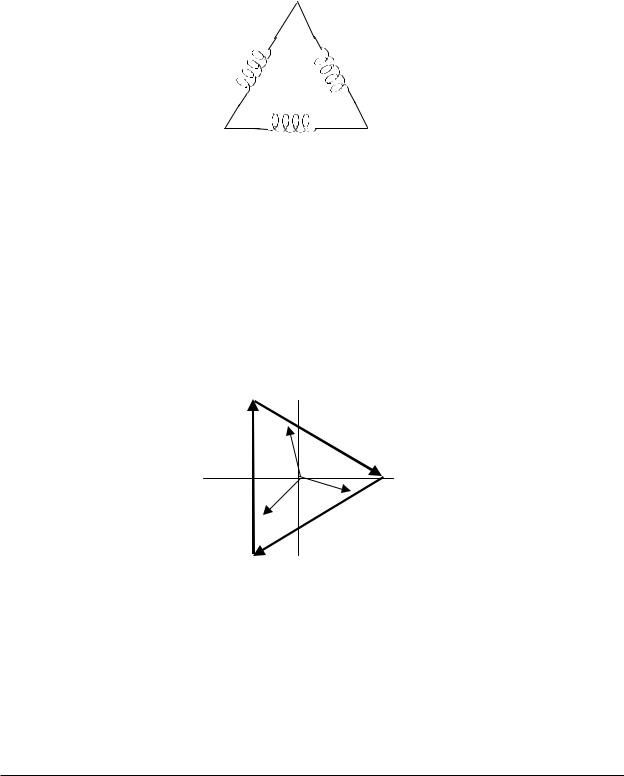
1.1.2: Delta Connection

Delta connected services may be fed with either three wires or four wires. In a three-phase delta service the load windings are connected from phase-to-phase rather than from phase-to-ground. Figure 1.3 shows the physical load connections for a delta service.

Phase C

Phase B	Phase A

Figure 1.3: Three-Phase Delta Winding Relationship

In this example of a delta service, three wires will transmit the power to the load. In a true delta service, the phase-to-ground voltage will usually not be balanced because the ground is not at the center of the delta.

Figure 1.4 shows the phasor relationships between voltage and current on a three-phase delta circuit.

In many delta services, one corner of the delta is grounded. This means the phase to ground voltage will be zero for one phase and will be full phase-to-phase voltage for the other two phases. This is done for protective purposes.

Vca

Ic

Vbc

Ia

Ib

Vab

Figure 1.4: Phasor Diagram, Three-Phase Voltages and Currents Delta Connected.

Another common delta connection is the four-wire, grounded delta used for lighting loads. In this connection the center point of one winding is grounded. On a 120/240 volt, four-wire, grounded delta service the phase-to-ground voltage would be 120 volts on two phases and 208 volts on the third phase. Figure 1.5 shows the phasor diagram for the voltages in a three-phase, four-wire delta system.

Electro Industries/GaugeTech Doc # E107706 V1.25

1-3

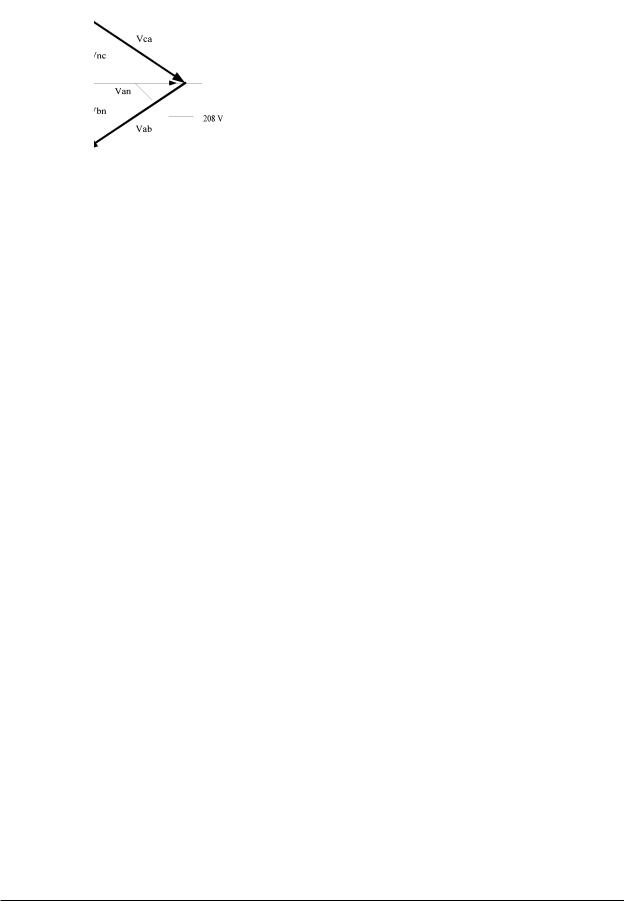
Fig 1.5: Phasor Diagram Showing Three-phase, Four-wire Delta Connected System

1.1.3: Blondell’s Theorem and Three Phase Measurement

In 1893 an engineer and mathematician named Andre E. Blondell set forth the first scientific basis for poly phase metering. His theorem states:

If energy is supplied to any system of conductors through N wires, the total power in the system is given by the algebraic sum of the readings of N wattmeters so arranged that each of the N wires contains one current coil, the corresponding potential coil being connected between that wire and some common point. If this common point is on one of the N wires, the measurement may be made by the use of N-1 wattmeters.

The theorem may be stated more simply, in modern language:

In a system of N conductors, N-1 meter elements will measure the power or energy taken provided that all the potential coils have a common tie to the conductor in which there is no current coil.

Three-phase power measurement is accomplished by measuring the three individual phases and adding them together to obtain the total three phase value. In older analog meters, this measurement was accomplished using up to three separate elements. Each element combined the single-phase voltage and current to produce a torque on the meter disk. All three elements were

arranged around the disk so that the disk was subjected to the combined torque of the three elements. As a result the disk would turn at a higher speed and register power supplied by each of the three wires.

According to Blondell's Theorem, it was possible to reduce the number of elements under certain conditions. For example, a three-phase, three-wire delta system could be correctly measured with two elements (two potential coils and two current coils) if the potential coils were connected between the three phases with one phase in common.

In a three-phase, four-wire wye system it is necessary to use three elements. Three voltage coils are connected between the three phases and the common neutral conductor. A current coil is required in each of the three phases.

In modern digital meters, Blondell's Theorem is still applied to obtain proper metering. The difference in modern meters is that the digital meter measures each phase voltage and current and calculates the single-phase power for each phase. The meter then sums the three phase powers to a

Electro Industries/GaugeTech Doc # E107706 V1.25

1-4

single three-phase reading.

Some digital meters calculate the individual phase power values one phase at a time. This means the meter samples the voltage and current on one phase and calculates a power value. Then it samples the second phase and calculates the power for the second phase. Finally, it samples the third phase and calculates that phase power. After sampling all three phases, the meter combines the three readings to create the equivalent three-phase power value. Using mathematical averaging techniques, this method can derive a quite accurate measurement of three-phase power.

More advanced meters actually sample all three phases of voltage and current simultaneously and calculate the individual phase and three-phase power values. The advantage of simultaneous sampling is the reduction of error introduced due to the difference in time when the samples were taken.

	C				Phase B
	B					Phase C

Node “n”

A				Phase A
N

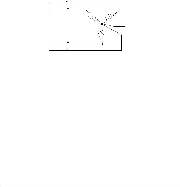
Figure 1.6: Three-Phase Wye Load illustrating Kirchhoff’s Law and Blondell’s Theorem

Blondell's Theorem is a derivation that results from Kirchhoff's Law. Kirchhoff's Law states that the sum of the currents into a node is zero. Another way of stating the same thing is that the current into a node (connection point) must equal the current out of the node. The law can be applied to measuring three-phase loads. Figure 1.6 shows a typical connection of a three-phase load applied to a threephase, four-wire service. Krichhoff's Laws hold that the sum of currents A, B, C and N must equal zero or that the sum of currents into Node "n" must equal zero.

If we measure the currents in wires A, B and C, we then know the current in wire N by Kirchhoff's Law and it is not necessary to measure it. This fact leads us to the conclusion of Blondell's Theorem that we only need to measure the power in three of the four wires if they are connected by a common node. In the circuit of Figure 1.6 we must measure the power flow in three wires. This will require three voltage coils and three current coils (a three element meter). Similar figures and conclusions could be reached for other circuit configurations involving delta-connected loads.

Electro Industries/GaugeTech Doc # E107706 V1.25

1-5

1.2: Power, Energy and Demand

It is quite common to exchange power, energy and demand without differentiating between the three. Because this practice can lead to confusion, the differences between these three measurements will be discussed.

Power is an instantaneous reading. The power reading provided by a meter is the present flow of watts. Power is measured immediately just like current. In many digital meters, the power value is actually measured and calculated over a one second interval because it takes some amount of time to calculate the RMS values of voltage and current. But this time interval is kept small to preserve the instantaneous nature of power.

Energy is always based on some time increment; it is the integration of power over a defined time increment. Energy is an important value because almost all electric bills are based, in part, on the amount of energy used.

Typically, electrical energy is measured in units of kilowatt-hours (kWh). A kilowatt-hour represents a constant load of one thousand watts (one kilowatt) for one hour. Stated another way, if the power delivered (instantaneous watts) is measured as 1,000 watts and the load was served for a one hour time interval then the load would have absorbed one kilowatt-hour of energy. A different load may have a constant power requirement of 4,000 watts. If the load were served for one hour it would absorb four kWh. If the load were served for 15 minutes it would absorb ¼ of that total or one kWh.

Figure 1.7 shows a graph of power and the resulting energy that would be transmitted as a result of the illustrated power values. For this illustration, it is assumed that the power level is held constant for each minute when a measurement is taken. Each bar in the graph will represent the power load for the one-minute increment of time. In real life the power value moves almost constantly.

The data from Figure 1.7 is reproduced in Table 2 to illustrate the calculation of energy. Since the time increment of the measurement is one minute and since we specified that the load is constant over that minute, we can convert the power reading to an equivalent consumed energy reading by multiplying the power reading times 1/60 (converting the time base from minutes to hours).

Kilowatts

100

80

60

40

20

Time (minutes) Æ

Figure 1.7: Power Use Over Time

Electro Industries/GaugeTech Doc # E107706 V1.25

1-6

	Time Interval	Power (kW)	Energy (kWh)	Accumulated
	(Minute)			Energy (kWh)
	1	30	0.50	0.50
	2	50	0.83	1.33
	3	40	0.67	2.00
	4	55	0.92	2.92
	5	60	1.00	3.92
	6	60	1.00	4.92
	7	70	1.17	6.09
	8	70	1.17	7.26
	9	60	1.00	8.26
	10	70	1.17	9.43
	11	80	1.33	10.76
	12	50	0.83	12.42
	13	50	0.83	12.42
	14	70	1.17	13.59
	15	80	1.33	14.92

Table 1.2: Power and Energy Relationship Over Time

As in Table 1.2, the accumulated energy for the power load profile of Figure 1.7 is 14.92 kWh.

Demand is also a time-based value. The demand is the average rate of energy use over time. The actual label for demand is kilowatt-hours/hour but this is normally reduced to kilowatts. This makes it easy to confuse demand with power. But demand is not an instantaneous value. To calculate demand it is necessary to accumulate the energy readings (as illustrated in Figure 1.7) and adjust the energy reading to an hourly value that constitutes the demand.

In the example, the accumulated energy is 14.92 kWh. But this measurement was made over a 15-minute interval. To convert the reading to a demand value, it must be normalized to a 60-minute interval. If the pattern were repeated for an additional three 15-minute intervals the total energy would be four times the measured value or 59.68 kWh. The same process is applied to calculate the 15-minute demand value. The demand value associated with the example load is 59.68 kWh/hr or 59.68 kWd. Note that the peak instantaneous value of power is 80 kW, significantly more than the demand value.

Electro Industries/GaugeTech Doc # E107706 V1.25

1-7

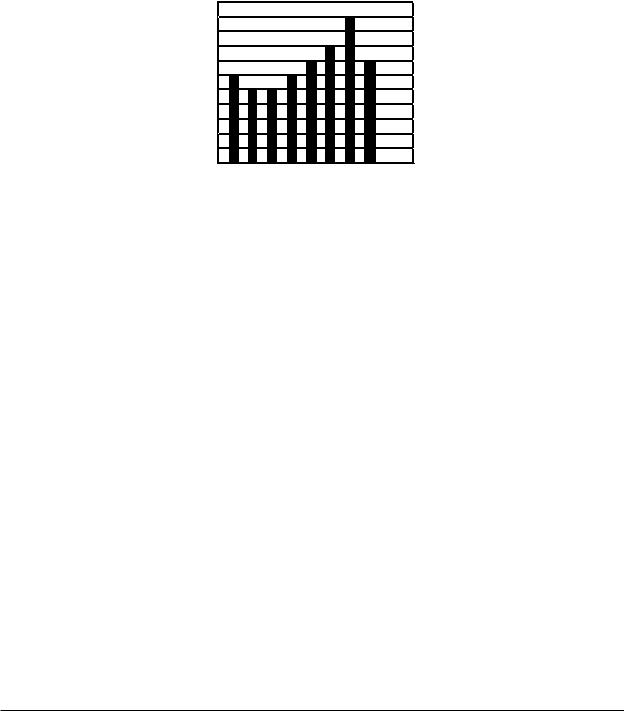
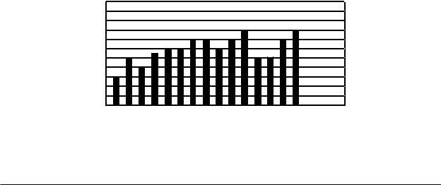
Figure 1.8 shows another example of energy and demand. In this case, each bar represents the energy consumed in a 15-minute interval. The energy use in each interval typically falls between 50 and 70 kWh. However, during two intervals the energy rises sharply and peaks at 100 kWh in interval number 7. This peak of usage will result in setting a high demand reading. For each interval shown the demand value would be four times the indicated energy reading. So interval 1 would have an associated demand of 240 kWh/hr. Interval 7 will have a demand value of 400 kWh/hr. In the data shown, this is the peak demand value and would be the number that would set the demand charge on the utility bill.

Kilowatt-hours

100

80

60

40

20

Intervals Æ

Figure 1.8: Energy Use and Demand

As can be seen from this example, it is important to recognize the relationships between power, energy and demand in order to control loads effectively or to monitor use correctly.

1.3: Reactive Energy and Power Factor

The real power and energy measurements discussed in the previous section relate to the quantities that are most used in electrical systems. But it is often not sufficient to only measure real power and energy. Reactive power is a critical component of the total power picture because almost all real-life applications have an impact on reactive power. Reactive power and power factor concepts relate to both load and generation applications. However, this discussion will be limited to analysis of reactive power and power factor as they relate to loads. To simplify the discussion, generation will not be considered.

Real power (and energy) is the component of power that is the combination of the voltage and the value of corresponding current that is directly in phase with the voltage. However, in actual practice the total current is almost never in phase with the voltage. Since the current is not in phase with the voltage, it is necessary to consider both the inphase component and the component that is at quadrature (angularly rotated 90o or perpendicular) to the voltage. Figure 1.9 shows a single-phase voltage and current and breaks the current into its in-phase and quadrature components.

Electro Industries/GaugeTech Doc # E107706 V1.25

1-8

	IR	V
IX	I	Angle θ

Figure 1.9: Voltage and Complex

The voltage (V) and the total current (I) can be combined to calculate the apparent power or VA. The voltage and the in-phase current (IR) are combined to produce the real power or watts. The voltage and the quadrature current (IX) are combined to calculate the reactive power.

The quadrature current may be lagging the voltage (as shown in Figure 1.9) or it may lead the voltage. When the quadrature current lags the voltage the load is requiring both real power (watts) and reactive power (VARs). When the quadrature current leads the voltage the load is requiring real power (watts) but is delivering reactive power (VARs) back into the system; that is VARs are flowing in the opposite direction of the real power flow.

Reactive power (VARs) is required in all power systems. Any equipment that uses magnetization to operate requires VARs. Usually the magnitude of VARs is relatively low compared to the real power quantities. Utilities have an interest in maintaining VAR requirements at the customer to a low value in order to maximize the return on plant invested to deliver energy. When lines are carrying VARs, they cannot carry as many watts. So keeping the VAR content low allows a line to carry its full capacity of watts. In order to encourage customers to keep VAR requirements low, most utilities impose a penalty if the VAR content of the load rises above a specified value.

A common method of measuring reactive power requirements is power factor. Power factor can be defined in two different ways. The more common method of calculating power factor is the ratio of the real power to the apparent power. This relationship is expressed in the following formula:

Total PF = real power / apparent power = watts/VA

This formula calculates a power factor quantity known as Total Power Factor. It is called Total PF because it is based on the ratios of the power delivered. The delivered power quantities will include the impacts of any existing harmonic content. If the voltage or current includes high levels of harmonic distortion the power values will be affected. By calculating power factor from the power values, the power factor will include the impact of harmonic distortion. In many cases this is the preferred method of calculation because the entire impact of the actual voltage and current are included.

A second type of power factor is Displacement Power Factor. Displacement PF is based on the angular relationship between the voltage and current. Displacement power factor does not consider the magnitudes of voltage, current or power. It is solely based on the phase angle differences. As a

Electro Industries/GaugeTech Doc # E107706 V1.25

1-9

result, it does not include the impact of harmonic distortion. Displacement power factor is calculated using the following equation:

Displacement PF = cos θ, where θ is the angle between the voltage and the current (see Fig. 1.9).

In applications where the voltage and current are not distorted, the Total Power Factor will equal the Displacement Power Factor. But if harmonic distortion is present, the two power factors will not be equal.

1.4: Harmonic Distortion

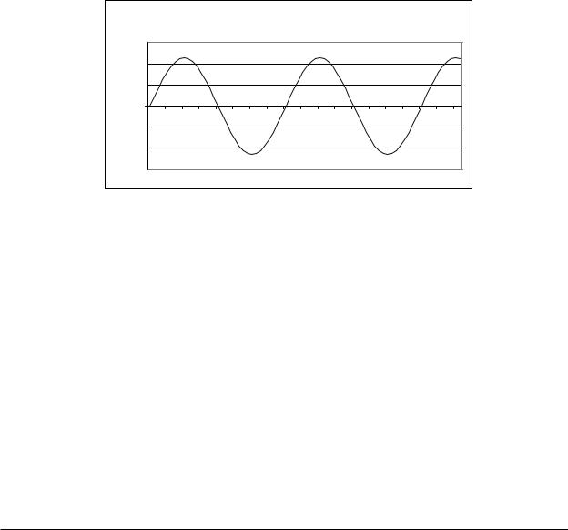
Harmonic distortion is primarily the result of high concentrations of non-linear loads. Devices such as computer power supplies, variable speed drives and fluorescent light ballasts make current demands that do not match the sinusoidal waveform of AC electricity. As a result, the current waveform feeding these loads is periodic but not sinusoidal. Figure 1.10 shows a normal, sinusoidal current waveform. This example has no distortion.

A Phase Current

1500
1000
500
0
-500	1	33	65
-1000
-1500

Figure 1.10: Nondistorted Current Waveform

Figure 1.11 shows a current waveform with a slight amount of harmonic distortion. The waveform is still periodic and is fluctuating at the normal 60 Hz frequency. However, the waveform is not a smooth sinusoidal form as seen in Figure 1.10.

Electro Industries/GaugeTech Doc # E107706 V1.25

1-10

Total A Phase Current with Harmonics

1500
1000
500
0
-500	1	33	65
-1000
-1500

Figure 1.11: Distorted Current Wave

The distortion observed in Figure 1.11 can be modeled as the sum of several sinusoidal waveforms of frequencies that are multiples of the fundamental 60 Hz frequency. This modeling is performed by mathematically disassembling the distorted waveform into a collection of higher frequency waveforms. These higher frequency waveforms are referred to as harmonics. Figure 1.12 shows the content of the harmonic frequencies that make up the distortion portion of the waveform in Figure 1.11.

							Expanded Harmonic Currents
	250
	200
	150
	100
Amps	50
	0	1	3	5	7	9
	-50						11	13	15	17	19	21	23	25	27	29	31	33	35	37	39
	-100
	-150
	-200
	-250
			2 Harmonic Current							3 Harmonic Current						5 Harmonic Current
			7 Harmonic Current							A Current Total Hrm

Figure 1.12: Waveforms of the Harmonics

The waveforms shown in Figure 1.12 are not smoothed but do provide an indication of the impact of combining multiple harmonic frequencies together.

When harmonics are present it is important to remember that these quantities are operating at higher frequencies. Therefore, they do not always respond in the same manner as 60 Hz values.

Electro Industries/GaugeTech Doc # E107706 V1.25

1-11

Inductive and capacitive impedance are present in all power systems. We are accustomed to thinking about these impedances as they perform at 60 Hz. However, these impedances are subject to frequency variation.

XL = jωL and

XC = 1/jωC

At 60 Hz, ω = 377; but at 300 Hz (5th harmonic) ω = 1,885. As frequency changes impedance changes and system impedance characteristics that are normal at 60 Hz may behave entirely different in presence of higher order harmonic waveforms.

Traditionally, the most common harmonics have been the low order, odd frequencies, such as the 3rd, 5th, 7th, and 9th. However newer, new-linear loads are introducing significant quantities of higher order harmonics.

Since much voltage monitoring and almost all current monitoring is performed using instrument transformers, the higher order harmonics are often not visible. Instrument transformers are designed to pass 60 Hz quantities with high accuracy. These devices, when designed for accuracy at low frequency, do not pass high frequencies with high accuracy; at frequencies above about 1200 Hz they pass almost no information. So when instrument transformers are used, they effectively filter out higher frequency harmonic distortion making it impossible to see.

However, when monitors can be connected directly to the measured circuit (such as direct connection to 480 volt bus) the user may often see higher order harmonic distortion. An important rule in any harmonics study is to evaluate the type of equipment and connections before drawing a conclusion. Not being able to see harmonic distortion is not the same as not having harmonic distortion.

It is common in advanced meters to perform a function commonly referred to as waveform capture. Waveform capture is the ability of a meter to capture a present picture of the voltage or current waveform for viewing and harmonic analysis. Typically a waveform capture will be one or two cycles in duration and can be viewed as the actual waveform, as a spectral view of the harmonic content, or a tabular view showing the magnitude and phase shift of each harmonic value. Data collected with waveform capture is typically not saved to memory. Waveform capture is a real-time data collection event.

Waveform capture should not be confused with waveform recording that is used to record multiple cycles of all voltage and current waveforms in response to a transient condition.

Electro Industries/GaugeTech Doc # E107706 V1.25

1-12

1.5: Power Quality

Power quality can mean several different things. The terms "power quality" and "power quality problem" have been applied to all types of conditions. A simple definition of "power quality problem" is any voltage, current or frequency deviation that results in mis-operation or failure of customer equipment or systems. The causes of power quality problems vary widely and may originate in the customer equipment, in an adjacent customer facility or with the utility.

In his book Power Quality Primer, Barry Kennedy provided information on different types of power quality problems. Some of that information is summarized in Table 1.3 below.

	Cause	Disturbance Type	Source
		Transient voltage disturbance,	Lightning
	Impulse Transient		Electrostatic discharge
		sub-cycle duration	Load switching
			Capacitor switching
	Oscillatory transient	Transient voltage, sub-cycle	Line/cable switching
			Capacitor switching
	with decay	duration
			Load switching
	Sag / swell	RMS voltage, multiple cycle	Remote system faults
		duration
			System protection
	Interruptions	RMS voltage, multiple second or	Circuit breakers
		longer duration	Fuses
			Maintenance
	Undervoltage /	RMS voltage, steady state,	Motor starting
		multiple second or longer	Load variations
	Overvoltage
		duration	Load dropping
		RMS voltage, steady state,	Intermittent loads
	Voltage flicker		Motor starting
		repetitive condition
			Arc furnaces
	Harmonic distortion	Steady state current or voltage,	Non-linear loads
		long term duration	System resonance

Table 1.3: Typical Power Quality Problems and Sources

It is often assumed that power quality problems originate with the utility. While it is true that may power quality problems can originate with the utility system, many problems originate with customer equipment. Customer-caused problems may manifest themselves inside the customer location or they may be transported by the utility system to another adjacent customer. Often, equipment that is sensitive to power quality problems may in fact also be the cause of the problem.

If a power quality problem is suspected, it is generally wise to consult a power quality professional for assistance in defining the cause and possible solutions to the problem.

Electro Industries/GaugeTech Doc # E107706 V1.25

1-13

Electro Industries/GaugeTech Doc # E107706 V1.25

1-14

Chapter 2

Nexus Overview

2.1: The Nexus System

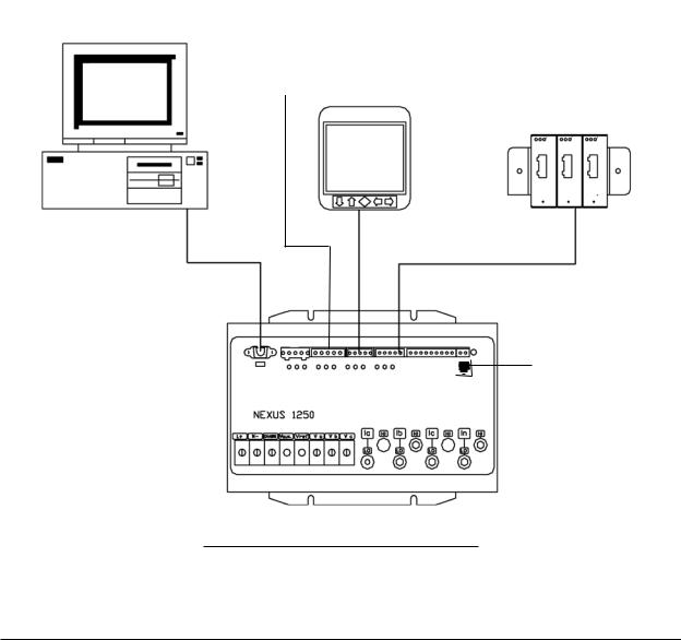
Electro Industries’ Nexus 1250/1252 combines high-end revenue metering with sophisticated power quality analysis. Its advanced monitoring capabilities provide detailed and precise pictures of any metered point within a distribution network. The P60N, P40N, P41N and P43N displays are detailed in Chapter 6. Extensive I/O capability is available in conjunction with all metering functions. The optional Communicator EXT software allows a user to poll and gather data from multiple Nexus meters installed at local or remote locations (see the Communicator EXT User Manual for details). On board mass memory enables the Nexus to retrieve and store multiple logs. The Nexus Meter with Internal Modem (or Network) Option connects to a PC via standard phone line (or MODBUS/TCP) and a daisy chain of Nexus Meters via an RS-485 connection. See Chapters 10 and 11 for details.

Modem/Ethernet

Option Modem Gateway or

Ethernet Gateway Computer RS-485 Connection or SCADA

System

Expandable I/O Modules

Nexus

Display

							Modem/Ethernet
							Option
							RJ-11 or RJ-45
		Nexus Meter
							Connection

Figure 2.1: The Nexus 1250/1252 System

e Electro Industries/GaugeTech Doc # E107706 V1.25

2-1

Nexus 1250/1252 Revenue Metering:

•Delivers laboratory-grade 0.04% Watt-hour accuracy in a field-mounted device.

•Autocalibrates when there is a temperature change of more than 10 degrees centigrade.

•Exceeds all ANSI C-12 and IEC 687 specifications.

•Adjusts for transformer and line losses, using user-defined compensation factors.

•Automatically logs time-of-use for up to eight programmable tariff registers.

•Counts pulses and aggregates different loads.

Nexus 1250/1252 Power Quality Monitoring:

•Records up to 512 samples per cycle on an event.

•Records sub-cycle transients on voltage or current readings.

•Measures and records Harmonics to the 83rd order.

•Offers inputs for neutral-to-ground voltage measurements.

•Synchronizes with IRIG-B clock signal.

Nexus 1250/1252 Memory, Communication and Control:

•Up to 4 Meg NVRAM.

•4 High Speed Communication Ports.

•Multiple Protocols (see section below on DNP V3.00).

•Built-in RTU functionality.

•Built-in PLC functionality.

•90msec High Speed Updates for Control.

2.2: DNP V3.00 Level 1 and Level 2

Nexus 1250 supports DNP V3.00 Level 1.

Nexus 1252 supports DNP V3.00 Level 2.

DNP Level 2 Features:

•Up to 136 measurement (64 Binary Inputs, 8 Binary Counters, 64 Analog Inputs) can be mapped to DNP Static Points (over 3000) in the customizable DNP Point Map.

•Up to 16 Relays and 8 Resets can be controlled through DNP Level 2.

•Report-by-Exception Processing (DNP Events) Deadbands can be set on a per-point basis.

•Freeze Commands: Freeze, Freeze/No-Ack, Freeze with Time, Freeze with Time/No-Ack.

•Freeze with Time Commands enable the Nexus meter to have internal time-driven Frozen and Frozen Event data. When the Nexus meter receives the Time and Interval, the data will be created.

For complete details, download the appropriate DNP User Manual from our website www.electroind.com.

2.3: Flicker

Nexus 1252 provides Flicker Evaluation in Instantaneous, Short Term and Long Term Forms. For a detailed explanation of Flicker, see Chapter 12 of this manual.

e Electro Industries/GaugeTech Doc # E107706 V1.25

2-2

2.4: INP2 Internal Modem with Dial-In/Dial-Out Option

2.4.1: Hardware Overview

The INP2 Option for the Nexus 1250/1252 meter provides a direct connection to a standard telephone line. No additional hardware is required to establish a communication connection between the meter and a remote computer. The RJ-11 Jack is on the face of the meter. A standard telephone RJ11 plug can connect the meter to a standard PSTN (Public Switched Telephone Network).

The modem operates at up to 56k baud. The modem supports both incoming calls (from a remote computer) and automatic dial-out calls when a defined event must be automatically reported.

With the device configured with the INP2 Option, the meter has dial-in capability and provides remote access to other Modbus-based serial devices via the meter’s RS-485 Gateway over your phone line. The meter will recognize and respond to a Modbus Address of 1. With any other address, the command will pass through the gateway and become a virtual connection between the Remote Modbus Master and any Modbus Slave connected to the RS-485 Gateway.

2.4.2: Dial-In Function

The modem continuously monitors the telephone line to detect an incoming call. When an incoming call is detected, the modem will wait a user-set number of rings and answer the call.

The modem can be programmed to check for a password on an incoming call. If the correct password is not provided the modem will hang up on the incoming call. If several unsuccessful incoming call attempts are received in a set time period, the modem will lock out future incoming calls for a user-set number of hours.

When an incoming call is successfully connected, the control of communications is passed to the calling software program. The modem will respond to computer commands to download data or other actions authorized by the meter passwords.

Refer to the Communicator EXT Software Manual for instructions on programming the modem.

2.4.3: Dial-Out Function

The Dial-Out Function (INP2) is intended to allow the meter to automatically report certain conditions without user intervention. The modem is normally polling the meter to determine if any abnormal or reportable conditions exist. The modem checks programmed meter conditions and programmed events (set in Nexus Communicator) to determine if a call should be placed.

If any of the monitored events exist, the modem will automatically initiate a call to a specified location to make a report or perform some other function. For log full conditions, the meter will automatically download the log(s) that are nearing the full state.

e Electro Industries/GaugeTech Doc # E107706 V1.25

2-3

2.5: Total Web Solutions

The 10/100BaseT Ethernet Option (INP 100) is a fully customizable web server that uses XML to provide access to real time data via Internet Explorer. EIG’s name for this dynamic system is Total Web Solutions. The system incorporates a highly programmable network card with built-in memory that is installed in the 100BaseT Option meters. Each card can be programmed to perform an extensive array of monitoring functions and the system is much faster than the 10BaseT Ethernet Option.

NOTE: Nexus meters with the INP10 Option do not support Total Web Solutions.

2.5.1: Hardware Overview

The Nexus 1250/1252 with the 10/100BaseT Ethernet Option (INP 100) has all the components of the standard Nexus 1250/1252 PLUS the capability of connection to a network through an Ethernet LAN or through the Internet via Modbus TCP, HTTP, SMTP, FTP and/or DHCP.

The Internal Network Option of the Nexus Meter is an extremely versatile communication tool.

•Adheres to IEEE 802.3 Ethernet standard using TCP/IP.

•Utilizes simple and inexpensive 100BaseT wiring and connections.

•Plugs right into your network using built-in RJ-45 jack.

•Programmable to any IP address, subnet mask and gateway requirements.

•Communicates using the industry standard Modbus/TCP protocol.

2.5.2: Hardware Connection

Use Standard RJ-45 10/100BaseT cable to connect with the Nexus. The RJ-45 line is inserted into the RJ-45 Port on the face of the Nexus with IMP100 Ethernet Option.

To make the software connection, use the following steps.

1.Using Port 1 or Port 4 (RS-485 connection), connect a PC to the meter. An RS-232/RS-485 Converter may be required (Example: Electro Industries Unicom 2500).

2.Double click on Communicator EXT Software to open.

3.Click the Quick Connect or the Connection Manager icon in the icon tool bar. Click the Serial Port button. Make sure data matches the meter then click Connect.

Set the Network Settings using the following steps:

(Refer to Section 3.6 of the Communicator EXT User Manual for more details).

1.From the Device Profile screen, double-click on the Communications Ports line, then double-click on any of the ports. The Device Profile Communications Settings screen appears.

e Electro Industries/GaugeTech Doc # E107706 V1.25

2-4

2. If you are going to use DHCP, click the Advanced Settings Button:

Click the tab at the top of the DHCP screen. Click Enable.

DHCP will automatically enter the IP Address and some or all of the Interface Settings. Click OK at the bottom of the screen to return to the Device Profile: Communication Ports screen. You may have to manually enter DNS, Email, Gateway Setting and/or a Unique Computer Name. Click OK.

3.If you are NOT using DHCP, in the Network Settings section, enter data provided by your systems manager:

IP Address:	10.0.0.1	(Example)
Subnet Mask:	255.255.255.0	(Example)
Default Gateway:	0.0.0.0	(Example)
Computer Name:	NETWORK	(Example)

Enter the Domain Name Server and Computer Name.

Customize Web Content, if desired. Default Pages with an extensive array of readings comes with the meter. The content of the pages can be customized using FTP Client.

From the Device Profile: Communications Ports screen, click Advanced Settings. Click the FTP Client tab on the top of the folder. Using FTP, you can easily replace any file by using the SAME FILE NAME as the one you want to replace.

Enter the Email Server IP Address. The Default Settings store ONE Email Server IP Address for administrative purposes or to send an alarm, if there is a problem. An ADDITIONAL 8 can be configured with FTP Client.

Update FIRMWARE, if needed, with TFTP protocol (see Appendix C).

After the above parameters are set, Communicator EXT will connect via the network using a Device Address of “1” and the assigned IP Address using the following steps:

1.Double click on Communicator EXT icon to open.

2.Click the Connect icon in the icon tool bar. The Connect screen will appear.

3.Click the Network button at the top of the screen. The screen will change to one requesting the following information:

Device Address:	1
Host:	IP Address (per your network administrator).
	Example: 10.0.0.1
Network Port:	502
Protocol:	Modbus TCP

4.Click the Connect button at the bottom of the screen. Communicator EXT connects to the Nexus with the Host IP Address via the Network.

e Electro Industries/GaugeTech Doc # E107706 V1.25

2-5

2.6: Measurements and Calculations

The Nexus 1250/1252 Meter measures many different power parameters. The following is a list of the formulas used to conduct calculations with samples for Wye and Delta services.

Samples for Wye: van, vbn, vcn, ia, ib, ic, in Samples for Delta: vab, vbc, vca, ia, ib, ic

Root Mean Square (RMS) of Phase to Neutral Voltages: n = number of samples

For Wye: x = an, bn, cn

n

∑vx2(t )

	VRMSx	=	t =1
			n

Root Mean Square (RMS) of Currents: n = number of samples

For Wye: x=a, b, c, n

For Delta: x = a, b, c

n

∑ix2(t )

	IRMSx	=	t =1
			n

Root Mean Square (RMS) of Phase to Phase Voltages: n = number of samples

For Wye: x, y= an, bn or bn, cn or cn, an

			n
			∑(vx(t ) − vy(t ) )2
	VRMSxy	=	t =1
			n

For Delta: xy = ab, bc, ca

n

∑vxy2 (t )

	VRMSxy	=	t =1
			n

e Electro Industries/GaugeTech Doc # E107706 V1.25

2-6